OU-HET 608 KEK-TH-1258 July 2008

${\cal N}=4$ Super Yang-Mills from the Plane Wave Matrix Model

Takaaki Ishii¹⁾, Goro Ishiki^1,2), Shinji Shimasaki¹⁾ and Asato Tsuchiya³⁾

¹⁾ Department of Physics, Graduate School of Science
Osaka University, Toyonaka, Osaka 560-0043, Japan
²⁾ Institute of Particle and Nuclear Studies
High Energy Accelerator Research Organization (KEK)
1-1 Oho, Tsukuba, Ibaraki 305-0801, Japan
³⁾ Department of Physics, Shizuoka University
836 Ohya, Suruga-ku, Shizuoka 422-8529, Japan

We propose a nonperturbative definition of ${\cal N}=4$ super Yang-Mills (SYM). We realize ${\cal N}=4$ SYM on $R\times S^{3}$ as the theory around a vacuum of the plane wave matrix model. Our regularization preserves sixteen supersymmetries and the gauge symmetry. We perform the 1-loop calculation to give evidences that the superconformal symmetry is restored in the continuum limit.

1 Introduction

The AdS/CFT correspondence [1, 2, 3], a typical example of which is a conjecture that type IIB superstring on $AdS_{5}\times S^{5}$ corresponds to ${\cal N}=4$ super Yang-Mills (SYM), has been intensively investigated for a decade. However, it has not been completely proven yet, partially because it is a strong/weak duality with respect to the coupling constants. It is, therefore, relevant to give a nonperturbative definition of ${\cal N}=4$ SYM that enables us to study its strong coupling regime. The lattice gauge theory is a promising candidate for such a nonperturbative definition. However, supersymmetric gauge theories on the lattice are generally difficult to construct, although there have been remarkable developments on this subject [4, 5, 6, 7, 8]. To give a nonperturbative definition of ${\cal N}=4$ SYM will not only bring enormous progress in the study of the AdS/CFT correspondence, but will also yield some insights into the problem of nonperturbative formulation of supersymmetric gauge theories.

It was shown in [9] that a gauge theory in the planar limit is equivalent to the matrix model (the reduced model) obtained by dimensionally reducing it to zero dimension if the $U(1)^{D}$ symmetry is unbroken, where $D$ stands for the dimensionality of space-time. This is the so-called large $N$ reduction. The global gauge symmetry of the matrix model is naturally interpreted as the local gauge symmetry of the original gauge theory. Thus, as an alternative to the lattice gauge theory, the matrix model may serve as a nonperturbative definition of the planar gauge theory with the gauge symmetry manifestly kept. The $U(1)^{D}$ symmetry is, however, spontaneously broken except for $D=2$, so that the above equivalence does not hold generically. There have been two improvements of the reduced model in which the $U(1)^{D}$ symmetry breaking is prevented so that the equivalence holds: one is the quenched reduced model [10, 11, 12, 13], and the other is the twisted reduced model [14]. These improved models work well for nonsupersymmetric planar gauge theories. It seems quite difficult to preserve supersymmetry manifestly in the twisted reduced model on the flat space and in the quenched reduced model, while the gauge symmetry is respected in both models.

The compactification in matrix models developed in [20] shares the same idea with the reduced model and will be called the matrix T-duality in this paper. While it is not restricted to the planar limit, it requires the size of matrices to be infinite from the beginning for the orbifolding condition to be imposed, so that it cannot be used to define any supersymmetric gauge theory nonperturbatively as it stands. It was argued in [4] that by imposing an orbifolding condition on the reduced model of a supersymmetric gauge theory, one can obtain its lattice theory in which part of the supersymmetries are manifestly preserved so that the fine-tuning of only a few parameters is required. This construction can be regarded as a finite-size matrix analog of the matrix T-duality. However, it has a problem of flat directions which is analogous to the problem of the $U(1)^{D}$ symmetry breaking. To overcome this problem, for instance, one needs to introduce a mass term for the scalar field, which leads to no preservation of supersymmetries.

In [21], Takayama and three of the present authors found the relationships among the $SU(2|4)$ symmetric theories, which include ${\cal N}=4$ SYM on $R\times S^{3}/Z_{k}$, 2+1 SYM on $R\times S^{2}$ [22] and the plane wave matrix model (PWMM) [23]. The last theory is obtained by consistently truncating the Kaluza-Klein modes of ${\cal N}=4$ SYM on $R\times S^{3}$ [24] and so are the former two theories [25]. In particular, 2+1 SYM on $R\times S^{2}$ and PWMM can be regarded as dimensional reductions of ${\cal N}=4$ SYM on $R\times S^{3}$. These theories possess common features: mass gap, discrete spectrum and many discrete vacua. From the gravity duals of those vacua proposed by Lin and Maldacena [25], the following relations among these theories are suggested: A) the theory around each vacuum of 2+1 SYM on $R\times S^{2}$ is equivalent to the theory around a certain vacuum of PWMM, and B) the theory around each vacuum of ${\cal N}=4$ SYM on $R\times S^{3}/Z_{k}$ is equivalent to the theory around a certain vacuum of 2+1 SYM on $R\times S^{2}$ with the orbifolding (periodicity) condition imposed. In [21], the relations A) and B) were shown directly on the gauge theory side. The results in [21] not only serve as a nontrivial check of the gauge/gravity correspondence for the $SU(2|4)$ theories, but they are also interesting from the point of view of the reduced model as follows. While there have been many works on realizing the gauge theories on the fuzzy sphere [26, 27, 28, 29] using matrix models [30, 31] and on the monopoles on the fuzzy sphere [31, 32, 33, 34, 36, 35], the relation A) shows that the continuum limit of the concentric fuzzy spheres with different radii corresponds to multiple monopoles. Note that realizing the gauge theories on the fuzzy sphere using the matrix models can be viewed as an extension of the twisted reduced model to curved space. The relation B) can be regarded as an extension of the matrix T-duality to that on a nontrivial $U(1)$ bundle, $S^{3}/Z_{k}$, whose base space is $S^{2}$. Indeed, the matrix T-duality was later extended to that on general $U(1)$ bundles in [37] and on general $SU(2)$ bundles in [38]. Combining the relations A) and B) leads to the relation C), that the theory around each vacuum of ${\cal N}=4$ SYM on $R\times S^{3}/Z_{k}$ is equivalent to the theory around a certain vacuum of PWMM with the orbifolding condition imposed. In particular, for $k=1$, ${\cal N}=4$ SYM on $R\times S^{3}$ is realized in PWMM. The possibility of defining ${\cal N}=4$ SYM in terms of PWMM nonperturbatively is suggested in [21]. The relationships shown in [21] are classical in the following sense: in the relation A), we show the equivalence at tree level and do not care about possible UV/IR mixing at higher orders, although the gravity duals suggest that any UV/IR mixing does not occur. In the relation B), the size of matrices must be infinite from the beginning as in the original matrix T-duality.

In this paper, we propose a nonperturbative definition of ${\cal N}=4$ SYM on $R\times S^{3}$ which is equivalently mapped to ${\cal N}=4$ SYM on $R^{4}$ at the conformal point and possesses the superconformal symmetry, the $SU(2,2|4)$ symmetry. We restrict ourselves to the planar limit. By referring to the relation C) in [21], we regularize ${\cal N}=4$ SYM on $R\times S^{3}$ nonperturbatively by using PWMM. Our analysis in this paper is quantum mechanical. The restriction to the planar limit enables us not to impose the orbifolding condition and to consider finite-size matrices such that the size of matrices plays the role of the ultraviolet cutoff. Thus we use an extension of the reduced model to curved space rather than the matrix T-duality to relate $2+1$ SYM on $R\times S^{2}$ to ${\cal N}=4$ SYM on $R\times S^{3}$. Because PWMM is a massive theory, there is no flat direction and the quenching prescription is not needed. Our regularization manifestly preserves the gauge symmetry and the $SU(2|4)$ symmetry, a subgroup of the $SU(2,2|4)$ symmetry. In particular, sixteen supersymmetries among thirty-two supersymmetries are respected in our regularization. The restriction to the planar limit and sixteen supersymmetries are probably sufficient to suppress the UV/IR mixing which may break the relation between $2+1$ SYM on $R\times S^{2}$ and PWMM quantum mechanically. They also stabilize the vacua of PWMM completely. Indeed, the gravity duals of these theories suggest $2+1$ SYM on $R\times S^{2}$ is obtained from PWMM quantum mechanically in the continuum limit at least in the planar limit. The full $SU(2,2|4)$ symmetry should be restored in the continuum limit. By performing the 1-loop analysis and comparing the results with those in continuum ${\cal N}=4$ SYM, we provide some evidences that our regularization of ${\cal N}=4$ SYM indeed works, although our final goal is to analyze ${\cal N}=4$ SYM nonperturbatively by using our formulation. Our theory still has the continuum time direction, which we need to cope with in order to put our theory on computer. For instance, we should be able to apply the method in [39, 40, 41] to our case. We comment on an interesting paper [42], the authors of which constructed the $S^{3}$ background in the IIB matrix model with the Myers term using the same procedure as [21]. They calculated the free energy of the theory around the background up to the 2-loop order to find the stability of the background. Note also that the authors of [43] discussed practicality of ${\cal N}=4$ SYM on the lattice recently.

This paper is organized as follows. In section 2, we study the large $N$ reduction on a finite volume. As an example, we consider the $\phi^{4}$ matrix quantum mechanics. We examine how the theory on $S^{1}$ is obtained from the matrix model that is its dimensional reduction to zero dimension, emphasizing the difference between the large $N$ reductions for the theories on $R$ and $S^{1}$. In section 3, we review the relationships among ${\cal N}=4$ SYM on $R\times S^{3}$, 2+1 SYM on $R\times S^{2}$ and PWMM shown in [21]. Based on these relationships and the result in section 2, we give a nonperturbative definition of ${\cal N}=4$ SYM on $R\times S^{3}$ using PWMM. In section 4, we perform the 1-loop calculation in our theory to give some evidences that our regularization of ${\cal N}=4$ SYM indeed works. Section 5 is devoted to conclusion and discussion. In appendices, some details are gathered.

2 The large $N$ reduction on finite volume

In this section, we study the large $N$ reduction on a finite volume, focusing on how different it is from that on an infinite volume. Let us consider a matrix quantum mechanics, whose action is given by

$$S=\int\>d\tau\mbox{Tr}\left(\frac{1}{2}\left(\frac{d\phi}{d\tau}\right)^{2}+\frac{1}{2}m^{2}\phi^{2}+\frac{1}{4}g^{2}\phi^{4}\right),$$ (2.1)

where $\phi(\tau)$ is an $N\times N$ hermitian matrix. We take the ’t Hooft limit: $N\rightarrow\infty,\;\;\lambda=g^{2}N=\mbox{fixed}$. First, we consider the case in which the theory is defined on $R$, namely $-\infty<\tau<\infty$. The prescription of the large $N$ reduction is to make the following replacement [11, 12, 13]:

$$\phi(\tau)\rightarrow e^{iP\tau}\phi e^{-iP\tau},$$

$$\int d\tau\rightarrow\frac{2\pi}{\Lambda},$$ (2.2)

where $\phi$ in the right-hand side of the first equation is no longer dependent on $\tau$ and $\Lambda$ is an ultraviolet cutoff. $P$ is a constant $N\times N$ matrix given by

$$P=\mbox{diag}(p_{1},p_{2},\cdots,p_{N})$$ (2.3)

with $p_{i}=\frac{\Lambda}{N}(i-\frac{N}{2})$. We take the limit in which

$$\Lambda\rightarrow\infty,\;\;N\rightarrow\infty,\;\;\Lambda/N\rightarrow 0.$$ (2.4)

Note that $\Lambda/N$ is an infrared cutoff. The action (2.1) is reduced to

$$S_{R}=\frac{2\pi}{\Lambda}\left(\frac{1}{2}\sum_{i,j}((p_{i}-p_{j})^{2}+m^{2})|\phi_{ij}|^{2}+\frac{1}{4}g^{2}\mbox{Tr}(\phi^{4})\right).$$ (2.5)

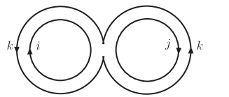
(a)

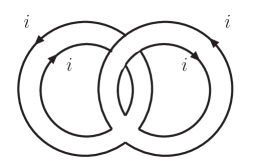
(b)

Figure 1: 2-loop diagrams for the free energy: (a)planar and (b)nonplanar

In order to illustrate the large $N$ reduction, we see that the free energy of the original model (2.1) agrees with that of the reduced model (2.5) at the two-loop level. There are two diagrams at the two-loop level for the free energy. Fig. 1-(a) shows the planar diagram while Fig. 1-(b) shows the nonplanar one. We evaluate the planar diagram in Fig. 1-(a) for the original model:

$$F^{2-loop}_{planar}/\mbox{Vol}=\frac{1}{2}N^{2}\lambda\int\frac{dpdq}{(2\pi)^{2}}\frac{1}{(p^{2}+m^{2})(q^{2}+m^{2})}.$$ (2.6)

The nonplanar diagram in Fig. 1-(b) for the original model is suppressed by the order of $1/N^{2}$ compared to the planar one in Fig. 1-(a). On the other hand, we evaluate the planar diagram in Fig. 1-(a) for the reduced model:

$$F^{2-loop}_{R,planar}/(2\pi/\Lambda) =\frac{1}{2}g^{2}\left(\frac{\Lambda}{2\pi}\right)^{2}\sum_{i,j,k}\frac{1}{((p_{i}-p_{k})^{2}+m^{2})((p_{j}-p_{k})^{2}+m^{2})}$$

$$=\frac{1}{2}g^{2}\left(\frac{\Lambda}{2\pi}\right)^{2}N\sum_{i,j}\frac{1}{(p_{i}^{2}+m^{2})(p_{j}^{2}+m^{2})}.$$ (2.7)

By using the relation valid in the limit (2.4),

$$\frac{\Lambda}{N}\sum_{i}f\left(\frac{\Lambda}{N}\left(i-\frac{N}{2}\right)\right)=\int_{-\infty}^{\infty}dpf(p),$$ (2.8)

one can easily verify that $F^{2-loop}_{planar}/\mbox{Vol}=F^{2-loop}_{R,planar}/(2\pi/\Lambda)$. Indeed, one can prove that $F_{planar}/\mbox{Vol}=F_{R,planar}/(2\pi/\Lambda)$ holds at all orders. We further evaluate the nonplanar diagram in Fig. 1-(b) for the reduced model:

$$F^{2-loop}_{R,nonplanar}/(2\pi/\Lambda) =\frac{1}{4}g^{2}\left(\frac{\Lambda}{2\pi}\right)^{2}\sum_{i}\frac{1}{m^{4}}$$

$$=\frac{1}{4}N^{2}\lambda\frac{1}{m^{4}}\times\left(\frac{\Lambda}{2\pi N}\right)^{2}.$$ (2.9)

Note that there is no correspondence for the nonplanar diagram between the original and reduced models. The nonplanar contribution (2.9) is suppressed by the factor $(\Lambda/N)^{2}$ in the limit (2.4), relative to the planar contribution (2.7). All the nonplanar contributions are indeed suppressed relative to the planar contributions in the reduced model. The reduced model therefore reproduces the ’t Hooft (planar) limit of the original model.

Next, we compactify the $\tau$-direction to $S^{1}$ with the radius $R$. We evaluate the planar diagram in Fig. 1-(a) for the original model:

$$\tilde{F}^{2-loop}_{planar}=\frac{1}{2}N^{2}\tilde{\lambda}\sum_{n,l}\frac{1}{(\frac{n^{2}}{R^{2}}+m^{2})(\frac{l^{2}}{R^{2}}+m^{2})},$$ (2.10)

where we take the $N\rightarrow\infty$ limit with $\tilde{\lambda}=g^{2}N/(2\pi R)$ fixed. Note that the nonplanar diagram in Fig. 1-(b) for the original model is still suppressed by $1/N^{2}$ relative to the planar diagram in Fig. 1-(a). Correspondingly, we consider the reduced model

$$\tilde{S}_{R}=\frac{1}{2}\sum_{i,j}((p_{i}-p_{j})^{2}+m^{2})|\phi_{ij}|^{2}+\frac{1}{4}g_{R}^{2}\mbox{Tr}(\phi^{4})$$ (2.11)

with $p_{i}=\frac{1}{R}\left(i-\frac{N}{2}\right)$. This naive reduced model turns out not to reproduce the original model on $S^{1}$. The contribution of the planar diagram in Fig. 1-(a) to the free energy for this reduced model is

$$\tilde{F}^{2-loop}_{R,planar} =\frac{1}{2}g_{R}^{2}\sum_{i,j,k}\frac{1}{(\frac{(i-k)^{2}}{R^{2}}+m^{2})(\frac{(j-k)^{2}}{R^{2}}+m^{2})}$$

$$=\frac{1}{2}g_{R}^{2}N\sum_{n,l}\frac{1}{(\frac{n^{2}}{R^{2}}+m^{2})(\frac{l^{2}}{R^{2}}+m^{2})},$$ (2.12)

while that of the nonplanar diagram in Fig. 1-(b) is

$$\tilde{F}^{2-loop}_{R,nonplanar}=\frac{1}{4}g_{R}^{2}\sum_{i}\frac{1}{m^{4}}=\frac{1}{4}g_{R}^{2}N\frac{1}{m^{4}}.$$ (2.13)

(2.13) is not suppressed relative to (2.12), because the infrared cutoff $1/R$ is finite in this case. Thus the correspondence between the original and reduced models fails in this case.

In the following, we modify the reduced model (2.5) to recover the correspondence. The action of the modified model takes the same form as (2.11) while $\phi$ is a $N(T+1)\times N(T+1)$ matrix, $i,j$ run from 1 to $N(T+1)$ and $p_{i}$ is given by the $i$-component of the matrix

$$\tilde{P}=\frac{1}{R}\mbox{diag}\left(-\frac{T}{2},-\frac{T}{2}+1,\cdots,\frac{T}{2}\right)\otimes 1_{N}.$$ (2.14)

Here $T$ is a positive even integer. We take the limit in which $T\rightarrow\infty,\;\;N\rightarrow\infty,\;\;\tilde{\lambda}=g_{R}^{2}N=\mbox{fixed}$. $T$ turns out to play the role of the ultraviolet cutoff for the momentum. In the modified model, the contribution of the planar diagram in Fig. 1-(a) to the free energy is

$$\tilde{F}^{2-loop}_{MR,planar} =\frac{1}{2}g_{R}^{2}N^{3}\sum_{a,b,c=-\frac{T}{2}}^{\frac{T}{2}}\frac{1}{(\frac{(a-c)^{2}}{R^{2}}+m^{2})(\frac{(b-c)^{2}}{R^{2}}+m^{2})}$$

$$=\frac{1}{2}N^{2}(T+1)\tilde{\lambda}\sum_{n,l}\frac{1}{(\frac{n^{2}}{R^{2}}+m^{2})(\frac{l^{2}}{R^{2}}+m^{2})}$$ (2.15)

Then, we see that $\tilde{F}^{2-loop}_{planar}=\tilde{F}^{2-loop}_{MR,planar}/(T+1)$. Indeed, it is easily verified that $\tilde{F}_{planar}=\tilde{F}_{MR,planar}/(T+1)$ holds at all orders. On the other hand, the contribution of the nonplanar diagram in Fig. 1-(b) to the free energy for the modified model is

$$\tilde{F}^{2-loop}_{MR,nonplanar}=\frac{1}{4}g_{R}^{2}N\sum_{a=-\frac{T}{2}}^{\frac{T}{2}}\frac{1}{m^{4}}=\frac{1}{4}(T+1)\tilde{\lambda}\frac{1}{m^{4}}.$$ (2.16)

This is suppressed by $1/N^{2}$ relative to (2.15). All the nonplanar contributions are indeed suppressed relative to the planar contributions in the modified model. Hence, the modified model reproduces the ’t Hooft (planar) limit of the original model on $S^{1}$.

For $D$-dimensional pure Yang-Mills (YM), the reduction analogous to (2.2) leads to

$$S_{YM}=\frac{1}{g^{2}}\int d^{D}x\frac{1}{4}\mbox{Tr}[\partial_{\mu}-iA_{\mu},\partial_{\nu}-iA_{\nu}]^{2}$$

$$\rightarrow S_{YM,R}=-\frac{2\pi}{\Lambda}\frac{1}{4g^{2}}\mbox{Tr}[P_{\mu}+A_{\mu},P_{\nu}+A_{\nu}]^{2},$$ (2.17)

where $P_{\mu}$ is the $D$-dimensional analogue of (2.3). It is known that the reduced model (2.17) does not reproduce the original YM, because the diagonal elements of $A_{\mu}$ are zero-dimensional massless fields and instable enough to absorb $P_{\mu}$. This is interpreted as the counterpart of the $U(1)^{D}$ symmetry breaking in the reduced model of the lattice gauge theory. Usually, in order to overcome this problem, the eigenvalues of $P_{\mu}+A_{\mu}$ in (2.17) are fixed to $P_{\mu}$ [12]. This is a quenching prescription. While the gauge symmetry is respected in this prescription, supersymmetry is not. In the case we are concerned with in this paper, we want to respect both symmetries simultaneously. We see how this problem is overcome in the next section.

3 Realization of ${\cal N}=4$ SYM on $R\times S^{3}$ in terms of PWMM

In this section, we review the relationships among ${\cal N}=4$ SYM on $R\times S^{3}$, 2+1 SYM on $R\times S^{2}$ and PWMM shown in [21], and we propose a nonperturbative definition of ${\cal N}=4$ SYM on $R\times S^{3}$, based on these relationships and the result in the previous section.

3.1 ${\cal N}=4$ SYM on $R\times S^{3}$ and the $SU(2|4)$ theories

The action of ${\cal N}=4$ SYM on $R\times S^{3}$ takes the form

$$S_{R\times S^{3}}=\frac{1}{g_{R\times S^{3}}^{2}}\int dt\frac{d\Omega_{3}}{(\mu/2)^{3}}\>\mbox{Tr}\left(-\frac{1}{4}F_{ab}F^{ab}-\frac{1}{2}D_{a}\Phi_{AB}D^{a}\Phi^{AB}-\frac{1}{2}\Phi_{AB}\Phi^{AB}\right.$$

$$\hskip 105.2751pt+\frac{1}{4}[\Phi_{AB},\Phi_{CD}][\Phi^{AB},\Phi^{CD}]+i\psi_{A}^{\dagger}D_{t}\psi^{A}+i\psi_{A}^{\dagger}\sigma^{i}D_{i}\psi^{A}$$

$$\hskip 105.2751pt\left.+\psi_{A}^{\dagger}\sigma^{2}[\Phi^{AB},(\psi_{B}^{\dagger})^{T}]-\psi^{AT}\sigma^{2}[\Phi_{AB},\psi^{B}]\right).$$ (3.1)

Here $a,b$ are the local Lorentz indices and run from 0 to 3. “0” corresponds to the time, $t$. $A,B$ are indices of the fundamental representation of $SU(4)$ and run from 1 to 4. $\Phi_{AB}=-\Phi_{BA}$ and $\Phi^{AB}=\frac{1}{2}\epsilon^{ABCD}\Phi_{CD}$ . The radius of $S^{3}$ is $2/\mu$. This theory possesses the superconformal symmetry, the $SU(2,2|4)$ symmetry. The action of 2+1 SYM on $R\times S^{2}$ takes the form

$$S_{R\times S^{2}}=\frac{1}{g_{R\times S^{2}}^{2}}\int dt\frac{d\Omega_{2}}{\mu^{2}}\mbox{Tr}\biggl{(}\frac{1}{2}(D_{t}\vec{X}-i\mu\vec{L}^{(0)}A_{t})^{2}-\frac{1}{2}(\mu\vec{X}+i(\mu\vec{L}^{(0)}\times\vec{X}-\vec{X}\times\vec{X}))^{2}$$

$$\hskip 71.13188pt+\frac{1}{2}D_{t}\Phi_{AB}D_{t}\Phi^{AB}+\frac{1}{2}\vec{{\cal D}}\Phi_{AB}\cdot\vec{{\cal D}}\Phi^{AB}-\frac{\mu^{2}}{8}\Phi_{AB}\Phi^{AB}+\frac{1}{4}[\Phi_{AB},\Phi_{CD}][\Phi^{AB},\Phi^{CD}]$$

$$\hskip 71.13188pt+i\psi_{A}^{\dagger}D_{t}\psi^{A}-\psi_{A}^{\dagger}\vec{\sigma}\cdot\vec{\cal D}\psi^{A}-\frac{3\mu}{4}\psi_{A}^{\dagger}\psi^{A}+\psi_{A}^{\dagger}\sigma^{2}[\Phi^{AB},(\psi_{B}^{\dagger})^{T}]-\psi^{AT}\sigma^{2}[\Phi_{AB},\psi^{B}]\biggr{)},$$ (3.2)

where

$$\vec{L}^{(0)}=-i\vec{e}_{\varphi}\partial_{\theta}+i\frac{1}{\sin\theta}\vec{e}_{\theta}\partial_{\varphi}$$ (3.3)

with $\vec{e}_{r}=(\sin\theta\cos\varphi,\sin\theta\sin\varphi,\cos\theta)$, $\vec{e}_{\theta}=\frac{\partial\vec{e}_{r}}{\partial\theta}$ and $\vec{e}_{\varphi}=\frac{1}{\sin\theta}\frac{\partial\vec{e}_{r}}{\partial\varphi}$, $\vec{{\cal D}}=\mu\vec{L}^{(0)}-[\vec{X},\;]$ and the radius of $S^{2}$ is $1/\mu$. The action of PWMM takes the form

$$S_{PW} =\frac{1}{g_{PW}^{2}}\int\frac{dt}{\mu^{2}}\>\mbox{Tr}\left(\frac{1}{2}(D_{t}X_{i})^{2}-\frac{1}{2}(\mu X_{i}-\frac{i}{2}\epsilon_{ijk}[X_{j},X_{k}])^{2}+\frac{1}{2}D_{t}\Phi_{AB}D_{t}\Phi^{AB}-\frac{\mu^{2}}{8}\Phi_{AB}\Phi^{AB}\right.$$

$$\qquad\qquad+\frac{1}{2}[X_{i},\Phi_{AB}][X_{i},\Phi^{AB}]+\frac{1}{4}[\Phi_{AB},\Phi_{CD}][\Phi^{AB},\Phi^{CD}]+i\psi_{A}^{\dagger}D_{t}\psi^{A}$$

$$\qquad\qquad\left.-\frac{3\mu}{4}\psi_{A}^{\dagger}\psi^{A}+\psi_{A}^{\dagger}\sigma^{i}[X_{i},\psi^{A}]+\psi_{A}^{\dagger}\sigma^{2}[\Phi^{AB},({\psi}_{B}^{\dagger})^{T}]-(\psi^{A})^{T}\sigma^{2}[\Phi_{AB},\psi^{B}]\right).$$ (3.4)

Both 2+1 SYM on $R\times S^{2}$ and PWMM possess the $SU(2|4)$ symmetry, which is a subgroup of the $SU(2,2|4)$ symmetry and has sixteen supercharges.

In the reminder of this section, for simplicity, we ignore the time component of the gauge field $A_{t}$ and the matter degrees of freedom, $\Phi_{AB}$ and $\psi^{A}$. It is easy to include these degrees of freedom in the arguments. All the statements in the following are also valid with these degrees of freedom.

3.2 $S^{3}$ and $S^{2}$

First, we summarize some useful facts about $S^{3}$ and $S^{2}$ (see also [38]). We regard $S^{3}$ as the $SU(2)$ group manifold. We parameterize an element of $SU(2)$ in terms of the Euler angles as

$$g=e^{-i\varphi\sigma_{3}/2}e^{-i\theta\sigma_{2}/2}e^{-i\psi\sigma_{3}/2},$$ (3.5)

where $0\leq\theta\leq\pi$, $0\leq\varphi<2\pi$, $0\leq\psi<4\pi$. The periodicity with respect to these angle variables is expressed as

$$(\theta,\varphi,\psi)\sim(\theta,\varphi+2\pi,\psi+2\pi)\sim(\theta,\varphi,\psi+4\pi).$$ (3.6)

The isometry of $S^{3}$ is $SO(4)=SU(2)\times SU(2)$, and these two $SU(2)$’s act on $g$ from left and right, respectively. Note that the superconformal group $SU(2,2|4)$ includes the $SO(4)$ group as a subgroup. We construct the right-invariant 1-forms,

$$dgg^{-1}=-i\mu E^{i}\sigma_{i}/2,$$ (3.7)

where the radius of $S^{3}$ is $2/\mu$. They are explicitly given by

$$E^{1}=\frac{1}{\mu}(-\sin\varphi d\theta+\sin\theta\cos\varphi d\psi),$$

$$E^{2}=\frac{1}{\mu}(\cos\varphi d\theta+\sin\theta\sin\varphi d\psi),$$

$$E^{3}=\frac{1}{\mu}(d\varphi+\cos\theta d\psi),$$ (3.8)

and satisfy the Maurer-Cartan equation

$$dE^{i}-\frac{\mu}{2}\epsilon_{ijk}E^{j}\wedge E^{k}=0.$$ (3.9)

The metric is constructed from $E^{i}$ as

$$ds^{2}=E^{i}E^{i}=\frac{1}{\mu^{2}}\left(d\theta^{2}+\sin^{2}\theta d\varphi^{2}+(d\psi+\cos\theta d\varphi)^{2}\right).$$ (3.10)

The Killing vectors dual to $E^{i}$ are given by

$${\cal{L}}_{i}=-\frac{i}{\mu}E^{M}_{i}\partial_{M},$$ (3.11)

where $M=\theta,\varphi,\psi$ and $E^{M}_{i}$ are inverse of $E^{i}_{M}$. The explicit form of the Killing vectors are

$${\cal{L}}_{1}=-i\left(-\sin\varphi\partial_{\theta}-\cot\theta\cos\varphi\partial_{\varphi}+\frac{\cos\varphi}{\sin\theta}\partial_{\psi}\right),$$

$${\cal{L}}_{2}=-i\left(\cos\varphi\partial_{\theta}-\cot\theta\sin\varphi\partial_{\varphi}+\frac{\sin\varphi}{\sin\theta}\partial_{\psi}\right),$$

$${\cal{L}}_{3}=-i\partial_{\varphi}.$$ (3.12)

Because of the Maurer-Cartan equation (3.9), the Killing vectors satisfy the SU(2) algebra, $[{\cal{L}}_{i},{\cal{L}}_{j}]=i\epsilon_{ijk}{\cal{L}}_{k}$.

One can also regard $S^{3}$ as a $U(1)$ bundle over $S^{2}=SU(2)/U(1)$. $S^{2}$ is parametrized by $\theta$ and $\varphi$ and covered with two local patches: the patch I defined by $0\leq\theta<\pi$ and the patch II defined by $0<\theta\leq\pi$. In the following expressions, the upper sign is taken in the patch I while the lower sign in the patch II. The element of $SU(2)$ in (3.5) is decomposed as

$$g=L\cdot h$$

$$\mbox{with}\;\;L=e^{-i\varphi\sigma_{3}/2}e^{-i\theta\sigma_{2}/2}e^{\pm i\varphi\sigma_{3}/2}\;\;\mbox{and}\;\;h=e^{-i(\psi\pm\varphi)\sigma_{3}/2}$$ (3.13)

$L$ represents an element of $S^{2}$, while $h$ represents the fiber $U(1)$. The fiber direction is parametrized by $y=\psi\pm\varphi$. Note that $L$ has no $\varphi$-dependence for $\theta=0,\pi$. The zweibein of $S^{2}$ is given by the $i=1,2$ components of the left-invariant 1-form, $-iL^{-1}dL=\mu e^{i}\sigma_{i}/2$ [45]. It takes the form

$$e^{1}=\frac{1}{\mu}(\pm\sin\varphi d\theta+\sin\theta\cos\varphi d\varphi),$$

$$e^{2}=\frac{1}{\mu}(-\cos\varphi d\theta\pm\sin\theta\sin\varphi d\varphi).$$ (3.14)

This zweibein gives the standard metric of $S^{2}$ with the radius $1/\mu$:

$$ds^{2}=\frac{1}{\mu^{2}}(d\theta^{2}+\sin^{2}\theta\varphi^{2}).$$ (3.15)

Making a replacement $\partial_{y}\rightarrow-iq$ in (3.12) leads to the angular momentum operator in the presence of a monopole with magnetic charge $q$ at the origin [46]:

$$L_{1}^{(q)}=i(\sin\varphi\partial_{\theta}+\cot\theta\cos\varphi\partial_{\varphi})-q\frac{1\mp\cos\theta}{\sin\theta}\cos\varphi,$$

$$L_{2}^{(q)}=i(-\cos\varphi\partial_{\theta}+\cot\theta\sin\varphi\partial_{\varphi})-q\frac{1\mp\cos\theta}{\sin\theta}\sin\varphi,$$

$$L_{3}^{(q)}=-i\partial_{\varphi}\mp q,$$ (3.16)

where $q$ is quantized as $q=0,\pm\frac{1}{2},\pm 1,\pm\frac{3}{2},\cdots$, because $y$ is a periodic variable with the period $4\pi$. These operators act on the local sections on $S^{2}$ and satisfy the $SU(2)$ algebra $[L_{i}^{(q)},L_{j}^{(q)}]=i\epsilon_{ijk}L_{k}^{(q)}$. Note that when $q=0$, these operators are reduced to the ordinary angular momentum operators (3.3) on $S^{2}$ (or $R^{3}$), which generate the isometry group of $S^{2}$, $SU(2)$. The $SU(2)$ acting on $g$ from left survives as the isometry of $S^{2}$. Note that in 2+1 SYM on $R\times S^{2}$ the isometry of $S^{2}$ is included in the $SU(2|4)$ symmetry as a subgroup.

3.3 Dimensional reductions

We dimensionally reduce the higher dimensional theories to the lower dimensional theories [24, 25, 37, 38]. We start with ${\cal N}=4$ SYM on $R\times S^{3}$:

$$S_{R\times S^{3}}=\frac{1}{g_{R\times S^{3}}^{2}}\int_{R\times S^{3}}\frac{1}{2}\mbox{Tr}(F\wedge\ast F).$$ (3.17)

We put $A=X_{i}E^{i}$ (note that we have ignored $A_{t}$). Then, the curvature 2-form is given by

$$F =dA-iA\wedge A$$

$$=\partial_{t}X_{i}dt\wedge E^{i}+i\mu{\cal L}_{i}X_{j}E^{i}\wedge E^{j}+X_{i}dE^{i}-iX_{i}X_{j}E^{i}\wedge E^{j}$$

$$=\partial_{t}X_{i}dt\wedge E^{i}+\frac{1}{2}\epsilon_{ijk}\left(\mu X_{k}+i\epsilon_{klm}(\mu{\cal L}_{l}X_{m}-\frac{1}{2}[X_{l},X_{m}])\right)E^{i}\wedge E^{j}.$$ (3.18)

By using (3.18), we rewrite (3.17) as

$$S_{R\times S^{3}}=\frac{1}{g_{R\times S^{3}}^{2}}\int dt\frac{d\Omega_{3}}{(\mu/2)^{3}}\mbox{Tr}\left(\frac{1}{2}(\partial_{t}X_{i})^{2}-\frac{1}{2}\left(\mu X_{i}+i\epsilon_{ijk}(\mu{\cal L}_{j}X_{k}-\frac{1}{2}[X_{j},X_{k}])\right)^{2}\right).$$ (3.19)

By dropping the $y$-derivatives in (3.19), we obtain 2+1 SYM on $R\times S^{2}$:

$$S_{R\times S^{2}}=\frac{1}{g_{R\times S^{2}}^{2}}\int dt\frac{d\Omega_{2}}{\mu^{2}}\mbox{Tr}\left(\frac{1}{2}(\partial_{t}X_{i})^{2}-\frac{1}{2}\left(\mu X_{i}+i\epsilon_{ijk}(\mu L^{(0)}_{j}X_{k}-\frac{1}{2}[X_{j},X_{k}])\right)^{2}\right),$$ (3.20)

where $g_{R\times S^{2}}^{2}=\frac{\mu g_{R\times S^{3}}^{2}}{4\pi}$. Thus we obtain 2+1 SYM on $R\times S^{2}$ from ${\cal N}=4$ SYM on $R\times S^{3}$ by dimensionally reducing the fiber direction of $S^{3}$ viewed as a $U(1)$ bundle over $S^{2}$. One of two $SU(2)$’s that are the isometry of $S^{3}$ survives as the isometry of $S^{2}$. Correspondingly, the superconformal symmetry, $SU(2,2|4)$, reduces to the $SU(2|4)$ symmetry. It is convenient for us to rewrite (3.20) using the gauge field and a Higgs field on $S^{2}$. We decompose $X_{i}$ into the components tangential and horizontal to $S^{2}$ [22]:

$$\vec{X}=\chi\vec{e}_{r}+a_{1}\vec{e}_{\varphi}-a_{2}\vec{e}_{\theta},$$ (3.21)

where $a_{1}$ and $a_{2}$ are the gauge field on $S^{2}$ and $\chi$ is the Higgs field on $S^{2}$. Substituting (3.21) into (3.20) leads to

$$S_{R\times S^{2}}=\frac{1}{g_{R\times S^{2}}^{2}}\int dt\frac{d\Omega_{2}}{\mu^{2}}\mbox{Tr}\left(\frac{1}{2}(\partial_{t}a_{a^{\prime}})^{2}+\frac{1}{2}(\partial_{t}\chi)^{2}-\frac{1}{2}(f_{12}-\mu\chi)^{2}-\frac{1}{2}(D_{a^{\prime}}\chi)^{2}\right),$$ (3.22)

where $a^{\prime}$ run from 1 to 2. Dropping all the derivatives in (3.20), we obtain

$$S_{PW}=\frac{1}{g_{PW}^{2}}\int\frac{dt}{\mu^{2}}\mbox{Tr}\left(\frac{1}{2}(\partial_{t}X_{i})^{2}-\frac{1}{2}\left(\mu X_{i}-\frac{i}{2}\epsilon_{ijk}[X_{j},X_{k}]\right)^{2}\right),$$ (3.23)

where $g_{PW}^{2}=\frac{g_{R\times S^{2}}^{2}}{4\pi}$. Thus PWMM is obtained from 2+1 SYM on $R\times S^{2}$ by a dimensional reduction. In this reduction, the $SU(2|4)$ symmetry is preserved.

3.4 Vacua

While ${\cal N}=4$ SYM on $R\times S^{3}$ possesses the unique vacuum, 2+1 SYM on $R\times S^{2}$ and PWMM possess many nontrivial vacua [23, 25]. Let us see how those vacua are described. First, the vacuum configurations of (3.22) with the gauge group $U(M)$ are determined by

$$f_{12}-\mu\chi=0,$$

$$D_{a^{\prime}}\chi=0.$$ (3.24)

In the gauge in which $\chi$ is diagonal, (3.24) is solved as

$$\hat{a}_{1}=0,$$

$$\hat{a}_{2}=-\frac{\cos\theta\mp 1}{\sin\theta}\hat{\chi},$$

$$\hat{\chi}=\mu\mbox{diag}(\cdots,\underbrace{q_{s-1},\cdots,q_{s-1}}_{N_{s-1}},\underbrace{q_{s},\cdots,q_{s}}_{N_{s}},\underbrace{q_{s+1},\cdots,q_{s+1}}_{N_{s+1}},\cdots),$$ (3.25)

where the gauge field takes the configurations of Dirac’s monopoles, so that $q_{s}$ must be half-integers due to Dirac’s quantization condition. Note also that $\sum_{s}N_{s}=M$. Thus the vacua of 2+1 SYM on $R\times S^{2}$ are classified by the monopole charges $q_{s}$ and their degeneracies $N_{s}$. The vacua preserve the $SU(2|4)$ symmetry. (3.24) is rewritten in terms of the notation in (3.20) as

$$\mu X_{i}+i\mu\epsilon_{ijk}L_{j}^{(0)}X_{k}-\frac{i}{2}\epsilon_{ijk}[X_{j},X_{k}]=0,$$ (3.26)

which is equivalent to

$$[\mu L_{i}^{(0)}-X_{i},\mu L_{j}^{(0)}-X_{j}]=i\mu\epsilon_{ijk}(\mu L_{k}^{(0)}-X_{k}),$$ (3.27)

and (3.25) is rewritten as

$$\mu L_{i}^{(0)}-\hat{X}_{i}=\mu\mbox{diag}(\cdots,\underbrace{L_{i}^{(q_{s-1})},\cdots,L_{i}^{(q_{s-1})}}_{N_{s-1}},\underbrace{L_{i}^{(q_{s})},\cdots,L_{i}^{(q_{s})}}_{N_{s}},\underbrace{L_{i}^{(q_{s+1})},\cdots,L_{i}^{(q_{s+1})}}_{N_{s+1}},\cdots),$$ (3.28)

where $\vec{\hat{X}}=\hat{\chi}\vec{e}_{r}+\hat{a}_{1}\vec{e}_{\varphi}-\hat{a}_{2}\vec{e}_{\theta}$.

Next, the vacuum configurations of (3.23) with the gauge group $U(\hat{M})$ are determined by

$$[X_{i},X_{j}]=-i\mu\epsilon_{ijk}X_{k}.$$ (3.29)

(3.29) is solved as

$$\hat{X}_{i}=-\mu L_{i},$$ (3.30)

where $L_{i}$ are the representation matrices of the $SU(2)$ generators which are in general reducible, and are decomposed into irreducible representations:

$$L_{i}=\begin{pmatrix}\rotatebox[origin={tl}]{-35.0}{$\cdots\;\;\;\overbrace{\rotatebox[origin={c}]{35.0}{$L_{i}^{[j_{s-1}]}$}\;\cdots\;\rotatebox[origin={c}]{35.0}{$L_{i}^{[j_{s-1}]}$}}^{\rotatebox{35.0}{$N_{s-1}$}}\;\;\;\overbrace{\rotatebox[origin={c}]{35.0}{$L_{i}^{[j_{s}]}$}\;\cdots\;\rotatebox[origin={c}]{35.0}{$L_{i}^{[j_{s}]}$}}^{\rotatebox{35.0}{$N_{s}$}}\;\;\;\overbrace{\rotatebox[origin={c}]{35.0}{$L_{i}^{[j_{s+1}]}$}\;\cdots\;\rotatebox[origin={c}]{35.0}{$L_{i}^{[j_{s+1}]}$}}^{\rotatebox{35.0}{$N_{s+1}$}}\;\;\;\cdots$}\end{pmatrix},$$ (3.31)

where $L_{i}^{[j]}$ are the spin $j$ representation matrices of $SU(2)$ and $\sum_{s}N_{s}(2j_{s}+1)=\hat{M}$. The vacua of the matrix model are classified by the $SU(2)$ representations $[j_{s}]$ and their degeneracies $N_{s}$. (3.31) represents concentric fuzzy spheres with different radii. The vacua preserve the $SU(2|4)$ symmetry.

3.5 Higher dimensional theories from lower dimensional theories

In what follows, we obtain the higher dimensional theories from the lower dimensional theories. First, we recall the relationship between the theory around (3.28) of $2+1$ SYM on $R\times S^{2}$ and the theory around (3.30) of PWMM, which was shown in [22] for the trivial vacuum of 2+1 SYM on $R\times S^{2}$ and in [21] for generic vacua. We introduce an ultraviolet cutoff $N_{0}$ and put

$$2q_{s}=2j_{s}+1-N_{0}$$ (3.32)

$$\frac{4\pi}{g_{R\times S^{2}}^{2}}=\frac{N_{0}}{g_{PW}^{2}}.$$ (3.33)

Then, the theory around (3.28) is equivalent to the theory around (3.30) in the limit in which $N_{0}\rightarrow\infty$ with $q_{s}$ and $g_{R\times S^{2}}$ fixed. The equivalence is proved as follows. We decompose the fields into the background corresponding to (3.28) and the fluctuation as $X_{i}^{(s,t)}\rightarrow\hat{X}_{i}^{(s,t)}+X_{i}^{(s,t)}$, where $(s,t)$ label the (off-diagonal) blocks. Note that $X_{i}^{(s,t)}$ is an $N_{s}\times N_{t}$ matrix. Then, (3.20) is expanded around (3.28) as

$$S_{R\times S^{2}} =\frac{1}{g_{R\times S^{2}}^{2}}\int dt\frac{d\Omega_{2}}{\mu^{2}}\frac{1}{2}\sum_{s,t}\mbox{tr}\left[\partial_{t}X_{i}^{(s,t)}\partial_{t}X_{i}^{(t,s)}\right.$$

$$\qquad\qquad\qquad\qquad-\left(\mu X_{i}^{(s,t)}+i\mu\epsilon_{ijk}L^{(q_{st})}_{j}X_{k}^{(s,t)}-\frac{i}{2}\epsilon_{ijk}[X_{j},X_{k}]^{(s,t)}\right)$$

$$\left.\qquad\qquad\qquad\quad\qquad\times\left(\mu X_{i}^{(t,s)}+i\mu\epsilon_{ilm}L^{(q_{ts})}_{l}X_{m}^{(t,s)}-\frac{i}{2}\epsilon_{ilm}[X_{l},X_{m}]^{(t,s)}\right)\right],$$ (3.34)

where

$$q_{st}=q_{s}-q_{t}.$$ (3.35)

We make a harmonic expansion of (3.34) by expanding the fluctuation in terms of the monopole vector spherical harmonics $\tilde{Y}_{Jmqi}^{\rho}$:

$$X_{i}^{(s,t)}=\sum_{\rho=0,\pm 1}\sum_{\tilde{Q}\geq|q_{st}|}\sum_{m=-Q}^{Q}x_{Jm\rho}^{(s,t)}\tilde{Y}_{Jmqi}^{\rho},$$ (3.36)

where $\rho$ stands for the polarization, $Q=J+\delta_{\rho 1}$ and $\tilde{Q}=J+\delta_{\rho-1}$. The properties of the monopole spherical harmonics are analyzed and summarized in [21, 38, 47] and references therein. Substituting (3.36) into (3.34) yields

$$S_{R\times S^{2}} =\frac{4\pi}{g_{R\times S^{2}}^{2}}\int\frac{dt}{\mu^{2}}\mbox{tr}\left[\frac{1}{2}\sum_{s,t}x_{Jm\rho}^{(s,t)\dagger}(\partial_{t}^{2}-\mu^{2}\rho^{2}(J+1)^{2})x_{Jm\rho}^{(s,t)}\right.$$

$$+i\mu\sum_{s,t,u}\rho_{1}(J_{1}+1){\cal E}_{J_{1}m_{1}q_{st}\rho_{1}\;J_{2}m_{2}q_{tu}\rho_{2}\;J_{3}m_{3}q_{us}\rho_{3}}x_{J_{1}m_{1}\rho_{1}}^{(s,t)}x_{J_{2}m_{2}\rho_{2}}^{(t,u)}x_{J_{3}m_{3}\rho_{3}}^{(u,s)}$$

$$+\frac{1}{2}\sum_{s,t,u,v}(-1)^{m-q_{su}+1}{\cal E}_{J-mq_{us}\rho\;J_{1}m_{1}q_{st}\rho_{1}\;J_{2}m_{2}q_{tu}\rho_{2}}{\cal E}_{Jmq_{su}\rho\;J_{3}m_{3}q_{uv}\rho_{3}\;J_{4}m_{4}q_{vs}\rho_{4}}$$

$$\left.\qquad\qquad\qquad\times x_{J_{1}m_{1}\rho_{1}}^{(s,t)}x_{J_{2}m_{2}\rho_{2}}^{(t,u)}x_{J_{3}m_{3}\rho_{3}}^{(u,v)}x_{J_{4}m_{4}\rho_{4}}^{(v,s)}\right],$$ (3.37)

where ${\cal E}_{J_{1}m_{1}q_{st}\rho_{1}\;J_{2}m_{2}q_{tu}\rho_{2}\;J_{3}m_{3}q_{us}\rho_{3}}$ is defined by

$${\cal E}_{J_{1}m_{1}q_{1}\rho_{1}J_{2}m_{2}q_{2}\rho_{2}J_{3}m_{3}q_{3}\rho_{3}}=\int\frac{d\Omega_{2}}{4\pi}\epsilon_{ijk}\tilde{Y}^{\rho_{1}}_{J_{1}m_{1}q_{1}i}\tilde{Y}^{\rho_{2}}_{J_{2}m_{2}q_{2}j}\tilde{Y}^{\rho_{3}}_{J_{3}m_{3}q_{3}k}$$

$$=\sqrt{6(2J_{1}+1)(2J_{1}+2\rho_{1}^{2}+1)(2J_{2}+1)(2J_{2}+2\rho_{2}^{2}+1)(2J_{3}+1)(2J_{3}+2\rho_{3}^{2}+1)}$$

$$\;\;\;\times(-1)^{-\frac{\rho_{1}+\rho_{2}+\rho_{3}+1}{2}}\left\{\begin{array}[]{ccc}Q_{1}&\tilde{Q}_{1}&1\\ Q_{2}&\tilde{Q}_{2}&1\\ Q_{3}&\tilde{Q}_{3}&1\end{array}\right\}\left(\begin{array}[]{ccc}Q_{1}&Q_{2}&Q_{3}\\ m_{1}&m_{2}&m_{3}\end{array}\right)\left(\begin{array}[]{ccc}\tilde{Q}_{1}&\tilde{Q}_{2}&\tilde{Q}_{3}\\ q_{1}&q_{2}&q_{3}\end{array}\right),$$ (3.45)

and we have used the equality

$$i\epsilon_{ijk}L_{j}^{(q)}\tilde{Y}^{\rho}_{Jmqk}+\tilde{Y}^{\rho}_{Jmqi}=\rho(J+1)\tilde{Y}^{\rho}_{Jmqi}.$$ (3.46)

Similarly, decomposing the matrices into the background given by (3.30) and the fluctuation as $X_{i}\rightarrow\hat{X}_{i}+X_{i}$ leads to the theory around (3.30):

$$S_{PW} =\frac{N_{0}}{g_{PW}^{2}}\int\frac{dt}{\mu^{2}}\frac{1}{2}\sum_{s,t}\mbox{tr}\left[\partial_{t}X_{i}^{(s,t)}\partial_{t}X_{i}^{(t,s)}-\left(\mu X_{i}^{(s,t)}+i\mu\epsilon_{ijk}L_{j}\circ X_{k}^{(s,t)}-\frac{i}{2}\epsilon_{ijk}[X_{j},X_{k}]^{(s,t)}\right)\right.$$

$$\left.\qquad\qquad\qquad\qquad\qquad\times\left(\mu X_{i}^{(t,s)}+i\mu\epsilon_{ilm}L_{l}\circ X_{m}^{(t,s)}-\frac{i}{2}\epsilon_{ilm}[X_{l},X_{m}]^{(t,s)}\right)\right],$$ (3.47)

where $L_{i}\circ$ is defined by

$$L_{i}\circ X_{j}^{(s,t)}=L_{i}^{[j_{s}]}X_{j}^{(s,t)}-X_{j}^{(s,t)}L_{i}^{[j_{t}]}.$$ (3.48)

The gauge symmetry of the above theory is expressed as

$$\delta X_{i}^{(s,t)}=i\mu L_{i}\circ\alpha^{(s,t)}-i[X_{i},\alpha]^{(s,t)}.$$ (3.49)

We make a harmonic expansion of (3.47) by expanding the fluctuation in terms of the fuzzy vector spherical harmonics $\hat{Y}_{Jm(j_{s}j_{t})i}^{\rho}$ defined in appendix A as

$$X_{i}^{(s,t)}=\sum_{\rho=0,\pm 1}\sum_{\tilde{Q}\geq|j_{s}-j_{t}|}^{j_{s}+j_{t}}\sum_{m=-Q}^{Q}x_{Jm\rho}^{(s,t)}\otimes\hat{Y}_{Jm(j_{s}j_{t})i}^{\rho}.$$ (3.50)

$x_{Jm\rho}^{(s,t)}$ in (3.50) is an $N_{s}\times N_{t}$ matrix. Since $j_{s}+j_{t}=N_{0}+q_{s}+q_{t}-1$, $N_{0}$ plays the role of the ultraviolet cutoff. Note also that $j_{s}-j_{t}=q_{s}-q_{t}=q_{st}$. Substituting (3.50) into (3.47) yields

$$S_{PW} =\frac{N_{0}}{g_{PW}^{2}}\int\frac{dt}{\mu^{2}}\mbox{tr}\left[\frac{1}{2}\sum_{s,t}x_{Jm\rho}^{(s,t)\dagger}(\partial_{t}^{2}-\rho^{2}(J+1)^{2})x_{Jm\rho}^{(s,t)}\right.$$

$$+i\mu\sum_{s,t,u}\rho_{1}(J_{1}+1)\hat{{\cal E}}_{J_{1}m_{1}(j_{s}j_{t})\rho_{1}\;J_{2}m_{2}(j_{t}j_{u})\rho_{2}\;J_{3}m_{3}(j_{u}j_{s})\rho_{3}}x_{J_{1}m_{1}\rho_{1}}^{(s,t)}x_{J_{2}m_{2}\rho_{2}}^{(t,u)}x_{J_{3}m_{3}\rho_{3}}^{(u,s)}$$

$$+\frac{1}{2}\sum_{s,t,u,v}(-1)^{m-q_{su}+1}\hat{{\cal E}}_{J-m(j_{u}j_{s})\rho\;J_{1}m_{1}(j_{s}j_{t})\rho_{1}\;J_{2}m_{2}(j_{t}j_{u})\rho_{2}}\hat{{\cal E}}_{Jm(j_{s}j_{u})\rho\;J_{3}m_{3}(j_{u}j_{v})\rho_{3}\;J_{4}m_{4}(j_{v}j_{s})\rho_{4}}$$

$$\left.\qquad\qquad\qquad\times x_{J_{1}m_{1}\rho_{1}}^{(s,t)}x_{J_{2}m_{2}\rho_{2}}^{(t,u)}x_{J_{3}m_{3}\rho_{3}}^{(u,v)}x_{J_{4}m_{4}\rho_{4}}^{(v,s)}\right],$$ (3.51)

where $\hat{{\cal E}}_{J_{1}m_{1}(jj^{\prime})\rho_{1}J_{2}m_{2}(j^{\prime}j^{\prime\prime})\rho_{2}J_{3}m_{3}(j^{\prime\prime}j)\rho_{3}}$ is defined in (A.18) and we have used (A.12). In the $N_{0}\rightarrow\infty$ limit, the ultraviolet cutoff goes to infinity and

$$\hat{{\cal E}}_{J_{1}m_{1}(j_{s}j_{t})\rho_{1}\;J_{2}m_{2}(j_{t}j_{u})\rho_{2}\;J_{3}m_{3}(j_{u}j_{s})\rho_{3}}\rightarrow{\cal E}_{J_{1}m_{1}q_{st}\rho_{1}\;J_{2}m_{2}q_{tu}\rho_{2}\;J_{3}m_{3}q_{us}\rho_{3}}$$ (3.52)

because the 6-j symbol behaves asymptotically for $R\gg 1$ as [48]

$$\left\{\begin{array}[]{ccc}a&b&c\\ d+R&e+R&f+R\\ \end{array}\right\}\approx\frac{(-1)^{a+b+c+2(d+e+f+R)}}{\sqrt{2R}}\left(\begin{array}[]{ccc}a&b&c\\ e-f&f-d&d-e\\ \end{array}\right).$$ (3.53)

Namely, this limit corresponds to the commutative (continuum) limit of the fuzzy spheres. Hence, in the $N_{0}\rightarrow\infty$ limit with $g_{PW}^{2}/N_{0}=g_{R\times S^{2}}^{2}/(4\pi)$ and $q_{s}=j_{s}-\frac{N_{0}}{2}+\frac{1}{2}$ fixed, (3.51) agrees with (3.37). We have proven our statement.

This equivalence is classical in the following sense. The asymptotic formula (3.53) holds for $a,b,c\ll R$. Namely, the reduction (3.52) is valid for $J_{1},J_{2},J_{3}\ll N_{0}$. Thus the equivalence is true at tree level. The loop effect may cause a deviation between the two theories quantum mechanically, since in the loop $J_{1},J_{2},J_{3}$ can be ${\cal O}(N_{0})$. Part of this deviation should be attributed to the UV/IR mixing. Suppose we restrict ourselves to the planar limit, in which $N_{s}\rightarrow\infty$ with $g_{R\times S^{2}}^{2}N_{s}$ fixed. Then, this restriction and sixteen supersymmetries are probably sufficient to suppress the UV/IR mixing, namely the noncommutativity in the continuum limit. Furthermore, as we discuss later, they completely stabilize the vacua of PWMM. Thus, the equivalence should also hold at the quantum level. Indeed, the gravity duals of 2+1 SYM on $R\times S^{2}$ and PWMM proposed in [25] support this conjecture [51, 21]. In the next section, we give an evidence that the UV/IR mixing does not exist.

Next, we recall that the theory around a certain vacuum of 2+1 $U(M=N\times\infty)$ SYM on $R\times S^{2}$ with the orbifolding (periodicity) condition imposed is equivalent to $U(N)$ ${\cal N}=4$ SYM on $R\times S^{3}$, which was shown in [21] (See also [37, 38]). This is an extension of the matrix T-duality to that on a nontrivial fiber bundle, $S^{3}$ as a $U(1)$ bundle over $S^{2}$. The vacuum of 2+1 SYM on $R\times S^{2}$ we take is given by (3.28) in the $N_{0}\rightarrow\infty$ limit with $s$ running from $-\infty$ to $\infty$, $q_{s}=s/2$, $N_{s}=N$ and $\frac{4\pi}{\mu}g_{R\times S^{2}}^{2}=g_{R\times S^{3}}^{2}$. We decompose the fields on $S^{2}$ into the background and the fluctuation

$$X_{i}\rightarrow\hat{X}_{i}+X_{i}$$ (3.54)

and impose the periodicity (orbifolding) condition on the fluctuation

$$X_{i}^{(s+1,t+1)}=X_{i}^{(s,t)}\equiv X_{i}^{(s-t)}.$$ (3.55)

The fluctuations are gauge-transformed from the patch I to the patch II as [37]

$$X_{i}^{(s-t)}=e^{-i(s-t)\varphi}X_{i}^{(s-t)}.$$ (3.56)

We make the Fourier transformation for the fluctuations on each patch to construct the gauge field on the total space from:

$$X_{i}(t,\theta,\varphi,\psi) =\sum_{w}X_{i}^{(w)}(t,\theta,\varphi)e^{-i\frac{1}{2}wy}.$$ (3.57)

We see from (3.56) that the left-hand side of (3.57) is indeed independent of the patches. Using (3.57), we obtain

$$L_{i}^{(q_{st})}X_{j}^{(s,t)}(\theta,\varphi)=\frac{1}{4\pi}\int_{0}^{4\pi}dy{\cal L}_{i}X_{j}(\theta,\varphi,\psi)e^{i\frac{1}{2}(s-t)y},$$

$$(X_{i}(\theta,\varphi)X_{j}(\theta,\varphi))^{(s,t)}=\frac{1}{4\pi}\int_{0}^{4\pi}dyX_{i}(\theta,\varphi,\psi)X_{j}(\theta,\varphi,\psi)e^{i\frac{1}{2}(s-t)y},$$ (3.58)

and so on. Then, we see that (3.34) equals $\sum_{s}\times$ (3.17). We divide an overall factor $\sum_{s}$ to extract a single period and obtain $U(N)$ ${\cal N}=4$ SYM on $R\times S^{3}$. Of course, we can verify this equivalence by seeing the agreement of the harmonic expansions of the two theories. We expand $X_{i}(t,\theta,\varphi,\psi)$ in terms of the vector spherical harmonics on $S^{3}$, $Y_{Jm\tilde{m}i}^{\rho}(\theta,\varphi,\psi)$ (See [38, 47, 21, 44]):

$$X_{i}(t,\theta,\varphi,\psi)=\sum_{\rho=0,\pm 1}\sum_{J}\sum_{m=-Q}^{Q}\sum_{\tilde{m}=-\tilde{Q}}^{\tilde{Q}}x_{Jm\tilde{m}\rho}(t)Y_{Jm\tilde{m}i}^{\rho}(\theta,\varphi,\psi),$$ (3.59)

where $J$ run over all non-negative integers and half-integers. $Q=J+\delta_{\rho 1}$ and $\tilde{Q}=J+\delta_{\rho-1}$ are the spins for the two $SU(2)$’s of the isometry of $S^{3}$. Note that the $SU(2)$ whose spin is $\tilde{Q}$ is broken in (3.20). By using the equality

$$\tilde{Y}_{Jmqi}^{\rho}(\theta,\varphi)=e^{iqy}Y_{Jmqi}^{\rho}(\theta,\varphi,\psi),$$ (3.60)

we can easily show that the harmonic expansion of (3.19) agrees with (3.37)$/\sum_{s}$ in the present set-up with the correspondence

$$x_{Jm\rho}^{(s,t)}\leftrightarrow x_{Jm\frac{1}{2}(s-t)\rho}.$$ (3.61)

Namely, $\frac{1}{2}(s-t)$ is identified with $\tilde{m}$.

Combining the above two equivalences, we see that the theory around (3.30) of PWMM in the $N_{0}\rightarrow\infty$ limit, where $s$ runs from $-\infty$ to $\infty$, $2j_{s}+1=N_{0}+s$ and $N_{s}=N$, is equivalent to $U(N)$ ${\cal N}=4$ SYM on $R\times S^{3}$ if $g_{PW}^{2}/N_{0}$ is fixed to $\frac{g_{R\times S^{3}}^{2}\mu}{16\pi^{2}}$, the periodicity condition is imposed on the fluctuation and the overall factor $\Sigma_{s}$ is divided.

3.6 Proposal for a nonperturbative definition of ${\cal N}=4$ SYM

The relationship between ${\cal N}=4$ SYM on $R\times S^{3}$ and 2+1 SYM on $R\times S^{2}$ is again classical for the following reason, and so is the relationship between ${\cal N}=4$ SYM on $R\times S^{3}$ and PWMM. In order to construct a well-defined quantum theory, we need to introduce an ultraviolet cutoff to the momentum of the fiber direction, which corresponds to $w$ in (3.57). Namely, we should consider finite-size matrices by making $s,t$ run from $-T/2$ to $T/2$ with $T$ an ultraviolet cutoff. In this situation, however, the periodicity condition (3.55) is not compatible with the gauge invariance. In order to resolve this problem, referring to the result for the modified reduced model in the previous section, we discard the periodicity condition and take the limit in which $N_{0}\rightarrow\infty,\;T\rightarrow\infty,\;N\rightarrow\infty,\;T/N_{0}\rightarrow 0,\;\frac{g_{PW}^{2}N}{N_{0}}=\frac{g_{R\times S^{2}}^{2}N}{4\pi}=\frac{g_{R\times S^{3}}^{2}N\mu}{16\pi^{2}}=\mbox{fixed}$. In this case, the $S^{1}$ in the previous section corresponds to the fiber direction of $S^{3}$ viewed as a $U(1)$ bundle over $S^{2}$. Our theory is a one-dimensional massive theory, so the instability discussed in the last part of the previous section is suppressed. Moreover, the $SU(2|4)$ symmetry preserved by the vacuum (3.30) completely stabilizes the vacuum. Indeed, the result in [52] ensures the perturbative stability, and it is easily seen from the result in [53] that the nonperturbative instability via the tunneling to other vacua of PWMM caused by the instantons is suppressed in the $N\rightarrow\infty$ limit. Thus, we do not need any quenching, and we can respect the gauge symmetry and the $SU(2|4)$ symmetry, namely half of supersymmetries of ${\cal N}=4$ SYM on $R\times S^{3}$, simultaneously. Indeed, (3.49) should correspond to the gauge symmetry of ${\cal N}=4$ SYM on $R\times S^{3}$. The noncommutativity probably vanishes in the continuum limit as mentioned before.

To summarize, we propose a nonperturbative definition of ${\cal N}=4$ SYM on $R\times S^{3}$ as follows. We consider the theory around (3.30) of PWMM with

$$-T/2\leq s\leq T/2,$$

$$2j_{s}+1=N_{0}+s,$$

$$N_{s}=N.$$ (3.62)

We take the limit in which

$$N_{0}\rightarrow\infty,\;\;\;T\rightarrow\infty,\;\;\;N\rightarrow\infty,$$

$$\mbox{with}\;\;\frac{T}{N_{0}}\rightarrow 0\;\;\mbox{and}\;\;\frac{g_{PW}^{2}N}{N_{0}}=\frac{\mu}{16\pi^{2}}g_{R\times S^{3}}^{2}N=\mbox{fixed}.$$ (3.63)

Then, we obtain the ’t Hooft (planar) limit of ${\cal N}=4$ SYM on $R\times S^{3}$. The condition $T/N_{0}\rightarrow 0$ can be relaxed to $N_{0}-\frac{T}{2}\rightarrow\infty$ that should be required to obtain the continuum spheres. For simplicity of the analysis, we adopt the stronger condition $T/N_{0}\rightarrow 0$ in this paper. The result should not depend on how to take the limit. Our formulation preserves the gauge symmetry and the $SU(2|4)$ symmetry. It is, in particular, remarkable that it preserves sixteen supersymmetries. We need to check the restoration of the superconformal symmetry $SU(2,2|4)$ to verify that our formulation does work well. The restoration of the superconformal symmetry should imply that no UV/IR mixing occur. In the next section, we give some evidences for the restoration of the superconformal symmetry.

4 Perturbative analysis

In this section, we perform a perturbative expansion of the theory around (3.30) of PWMM. In the beginning, we do not assume (3.62) or (3.63). We make a replacement $X_{i}\rightarrow\hat{X}_{i}+X_{i}$ in (3.4). We adopt the Feynman-type gauge and add the following gauge fixing and Fadeev-Popov terms to the action:

$$\frac{1}{g_{PW}^{2}}\int\frac{dt}{\mu^{2}}\mbox{Tr}\left(-\frac{1}{2}(-\partial_{t}A_{t}+i\mu[L_{i},X_{i}])^{2}+i\bar{c}\partial_{t}D_{t}c+\mu\bar{c}[L_{i},i\mu[L_{i},c]-i[X_{i},c]]\right).$$ (4.1)

The resultant gauge-fixed action is written down in (B.1) in appendix B. The mode expansion of the fields is given in (B.6), which of course includes (3.50). The harmonic expansion of the gauge-fixed action is given in (B.7), (B.10) and (B.11) which are a counterpart of (3.51). One can read off the propagators from (B.7) as in (B.9) and the vertices from (B.10) and (B.11).

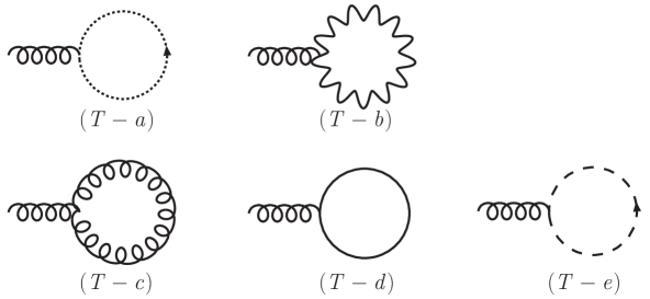
Figure 2: Tadpole diagrams. The curly line represents the propagator of $X_{i}$. The wavy line represents the propagator of $A_{t}$. The dotted line represents the propagator of the ghost. The solid line represents the propagator of $\Phi_{AB}$. The dashed line represents the propagator of $\psi^{A}$.

First, we calculate the 1-loop contribution to the tadpoles. The only possibly nonzero contribution is the truncated 1-point function for $x_{Jm\rho}^{(s,t)}(p)_{ij}$, where $i,j$ run from 1 to $N_{s}$ and $p$ is dual to $t$ in the Fourier transformation. This quantity takes the form

$$2\pi\delta(p)\delta_{st}\delta_{ij}\delta_{\rho\>-1}\delta_{J0}\delta_{m0}\delta_{ij}\Upsilon^{(s)}.$$ (4.2)

There are five 1-loop diagrams for this 1-point function as shown in Fig. 2. Note that all these diagrams are planar ones. The diagrams $(T-a)$ and $(T-b)$ completely cancel each other. Below we list the value of $\Upsilon^{(s)}$ for each of the remaining diagrams.

$$(T-c)=\frac{1}{2}g^{2}\sqrt{N_{0}}\sum_{t,R}N_{t}(-1)^{R+j_{s}+j_{t}}\sqrt{R(R+1)(2R+1)}(2R+1)$$

$$\qquad\qquad\qquad\qquad\qquad\times\left(\frac{2R+3}{(R+1)^{2}}+\frac{2R-1}{R^{2}}+\frac{1}{R^{3/2}(R+1)^{3/2}}\right){\scriptsize\begin{Bmatrix}1&R&R\\ j_{t}&j_{s}&j_{s}\end{Bmatrix}},$$ (4.3)

$$(T-d)=12g^{2}\sqrt{N_{0}}\sum_{t,R}N_{t}(-1)^{R+j_{s}+j_{t}}\sqrt{R(R+1)(2R+1)}{\scriptsize\begin{Bmatrix}1&R&R\\ j_{t}&j_{s}&j_{s}\end{Bmatrix}},$$ (4.4)

$$(T-e)=-\frac{4}{3}\times(T-d),$$ (4.5)

where $g^{2}=g_{PW}^{2}\mu^{2}/N_{0}$. The $6$-$j$ symbol in the above expressions can be written explicitly:

$${\scriptsize\begin{Bmatrix}1&R&R\\ j_{t}&j_{s}&j_{s}\end{Bmatrix}}=(-1)^{j_{t}+j_{s}+R+1}\frac{1}{2}\frac{(j_{s}-j_{t})(j_{s}+j_{t}+1)+R(R+1)}{\sqrt{j_{s}(j_{s}+1)(2j_{s}+1)R(R+1)(2R+1)}},$$ (4.6)

By using (4.6) and $j_{s}=\frac{N_{0}}{2}+q_{s}-\frac{1}{2}$, we sum up the contributions to the tadpole:

$$(T-c)+(T-d)+(T-e)$$

$$=g^{2}\sum_{t}N_{t}\sum_{R=|q_{s}-q_{t}|}^{N_{0}-1+q_{s}+q_{t}}F(R)\left((q_{s}-q_{t})+(R(R+1)+R\mbox{-independent terms})\times{\cal O}\left(\frac{1}{N_{0}}\right)\right),$$ (4.7)

where

$$F(R) =4-\frac{1}{2}(2R+1)\left(\frac{2R+3}{(R+1)^{2}}+\frac{2R-1}{R^{2}}+\frac{1}{R^{3/2}(R+1)^{3/2}}\right).$$ (4.8)

The first term in (4.8) comes from $(T-d)$ and $(T-e)$ while the second term from $(T-c)$. The asymptotic behavior of $F(R)$ for large $R$,

$$F(R)\sim\frac{3}{8R^{4}}+{\cal O}\left(\frac{1}{R^{5}}\right),$$ (4.9)

tells us that in the $N_{0}\rightarrow\infty$ limit

$$(T-c)+(T-d)+(T-e)=g^{2}\sum_{t}N_{t}\sum_{R=|q_{s}-q_{t}|}^{\infty}F(R)(q_{s}-q_{t})+{\cal O}\left(\frac{1}{N_{0}}\right).$$ (4.10)

We find no $N_{0}$-dependent divergences.

We see that

$$\sum_{s}N_{s}((T-c)+(T-d)+(T-e))=0.$$ (4.11)

This means that the vev of $\sum_{s,i}x_{Jm\rho}^{(s,s)}(p)_{ii}$ that corresponds to the one-point function for the overall $U(1)$ field on $R\times S^{2}$ indeed vanishes. This is consistent with the fact that it is a free field decoupled from the other fields when in the theory around (3.28) one takes the Feynman-like gauge, to which the gauge corresponding to (4.1) reduces naively in the $N_{0}\rightarrow\infty$ limit. One can easily verify from (4.8) that if there is no supersymmetry, the vev of the one-point function for the overall $U(1)$ field does not vanish. Note that this happens even with the restriction to the planar limit since all the tadpole diagrams in Fig. 2 are planar. In [54], the same phenomenon was observed in a bosonic gauge theory on the fuzzy sphere in the continuum limit and interpreted as the UV/IR mixing. On the other hand, by shifting $\mu$ in (3.30), one can always cancel the vev of the one point function for the overall U(1) field and might obtain the commutative gauge theory. However, in any case, we cannot follow this prescription because it breaks supersymmetry. Here we have obtained an evidence that in our case the UV/IR mixing is avoided, that is, the noncommutativity vanishes in the continuum limit, in a way compatible with supersymmetry.

If we consider the theory around (3.30) with (3.62) and (3.63) that would realize ${N=4}$ SYM on $R\times S^{3}$, we find no $T$-dependent divergences in (4.10). Furthermore, (4.10) vanishes for fixed $s$ in the $T\rightarrow\infty$ due to the summation over $t$. In this case, the gauge corresponding to (4.1) reduces naively in the limit (3.63) to the Feynman gauge in ${\cal N}=4$ SYM on $R\times S^{3}$. The isometry of $S^{3}$, $SO(4)=SU(2)\times SU(2)$, is manifest in ${\cal N}=4$ SYM on $R\times S^{3}$ with the Feynman gauge, and all the tadpoles vanish due to this isometry. The symmetry corresponding to one of the above two $SU(2)$’s already exists a priori in our theory, while the other does not. Vanishing of (4.10) is a signal for the restoration of the $SO(4)$ symmetry in the continuum limit (3.63). If this restoration and the vanishing of the noncommutativity is indeed the case, we obtain a commutative gauge theory with sixteen supersymmetries on $R\times S^{3}$. This theory should be nothing but ${\cal N}=4$ SYM on $R\times S^{3}$ unless we perform any extra fine-tunings. Thus we have found an evidence that the superconformal symmetry is restored and our formalism does work well.

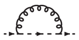
$(F-a)$

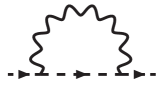
$(F-b)$

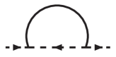
$(F-c)$

Figure 3: Diagrams for the one-loop self-energy of $\psi^{A}$. The curly line represents the propagator of $X_{i}$. The wavy line represents the propagator of $A_{t}$. The solid line represents the propagator of $\Phi_{AB}$. The dashed line represents the propagator of $\psi^{A}$.

Next, we calculate the fermion self-energy in the theory around (3.30) with (3.62) and (3.63) at the one-loop level, and compare the result in ${\cal N}=4$ SYM on $R\times S^{3}$. The fermion self-energy is given by the truncated two-point function $\langle\psi_{Jm\kappa}^{(s,t)A}(p)_{ij}\psi_{J^{\prime}m^{\prime}\kappa^{\prime}A^{\prime}}^{(s^{\prime},t^{\prime})\dagger}(p^{\prime})_{kl}\rangle$, and this takes the form

$$2\pi\delta(p-p^{\prime})\delta_{ss^{\prime}}\delta_{tt^{\prime}}\delta^{A}_{A^{\prime}}\delta_{il}\delta_{jk}\delta_{JJ^{\prime}}\delta_{mm^{\prime}}\Omega^{(s,t)}_{J\kappa\kappa^{\prime}}(p).$$ (4.12)

The diagrams which contribute to the fermion self-energy at the one-loop order are shown in Fig. 3. We list the value of $\Omega^{(s,t)}_{J\kappa\kappa^{\prime}}(p)$ for each diagram in appendix C.

We set the external indices to specific values to calculate the leading contribution in the continuum limit (3.63): $s=t=0$, $\kappa=\kappa^{\prime}=1$ and $J=0$. The divergent part of $\Omega_{011}^{(0,0)}(p)$ for each diagram is evaluated as

$$(F-a)_{\kappa=\kappa^{\prime}=1,J=0}$$

$$=-\frac{ig^{2}}{\mu^{2}}N\sum_{u=-\frac{T}{2}}^{\frac{T}{2}}\sum_{R_{1}=|\frac{u}{2}|}^{N_{0}-1+\frac{u}{2}}\Biggl{[}\frac{2R_{1}+3}{R_{1}+1}\cdot\frac{1}{l-(2R_{1}+\frac{7}{4})}+\frac{2R_{1}-1}{R_{1}}\cdot\frac{1}{l+(2R_{1}+\frac{1}{4})}$$

$$\quad+\sqrt{\frac{R_{1}}{R_{1}+1}}\cdot\frac{1}{l-\{R_{1}+\sqrt{R_{1}(R_{1}+1)}+\frac{3}{4}\}}+\sqrt{\frac{R_{1}+1}{R_{1}}}\cdot\frac{1}{l+\{R_{1}+\sqrt{R_{1}(R_{1}+1)}+\frac{1}{4}\}}\Biggr{]}$$

$$\sim-\frac{4ig^{2}}{\mu^{2}}N\left(-l-\frac{1}{4}\right)\ln T-\frac{4ig^{2}}{\mu^{2}}N\left(-\frac{l}{2}+\frac{5}{8}\right)\ln T,$$

$$(F-b)_{\kappa=\kappa^{\prime}=1,J=0}$$

$$=\frac{ig^{2}}{\mu^{2}}N\sum_{u=-\frac{T}{2}}^{\frac{T}{2}}\sum_{R_{1}=|\frac{u}{2}|}^{N_{0}-1+\frac{u}{2}}$$

$$\quad\times\Biggl{[}\sqrt{\frac{R_{1}+1}{R_{1}}}\cdot\frac{1}{l-\{R_{1}+\sqrt{R_{1}(R_{1}+1)}+\frac{3}{4}\}}+\sqrt{\frac{R_{1}}{R_{1}+1}}\cdot\frac{1}{l+\{R_{1}+\sqrt{R_{1}(R_{1}+1)}+\frac{1}{4}\}}\Biggr{]}$$

$$\sim-\frac{4ig^{2}}{\mu^{2}}N\left(\frac{l}{2}+\frac{3}{8}\right)\ln T,$$

$$(F-c)_{\kappa=\kappa^{\prime}=1,J=0}$$

$$=-\frac{12ig^{2}}{\mu^{2}}N\sum_{u=-\frac{T}{2}}^{\frac{T}{2}}\sum_{R_{1}=|\frac{u}{2}|}^{N_{0}-1+\frac{u}{2}}\Biggl{[}\frac{R_{1}+1}{2R_{1}+1}\cdot\frac{1}{l+(2R_{1}+\frac{5}{4})}+\frac{R_{1}}{2R_{1}+1}\cdot\frac{1}{l-(2R_{1}+\frac{3}{4})}\Biggr{]}$$

$$\sim-\frac{12ig^{2}}{\mu^{2}}N\left(-l+\frac{3}{4}\right)\ln T,$$ (4.13)

where $l=p/\mu$. Note that we find no $N_{0}$-dependent divergences in each diagram. This is consistent with the fact that (2+1)-dimensional gauge theory is super renormalizable. We find that the divergence in $T$ is logarithmic in each diagram. This is again consistent with the fact that the fermion self-energy has only the logarithmic divergence in four dimensions.

In ${\cal N}=4$ SYM on $R\times S^{3}$, the fermion self-energy is given by the two point function $\langle\psi^{A}_{Jm\tilde{m}\kappa}(p)_{ij}\psi^{\dagger}_{J^{\prime}m^{\prime}\tilde{m}^{\prime}\kappa^{\prime}A^{\prime}}(p^{\prime})_{kl}\rangle$, where $J$ and $\tilde{J}$ are the spins for the two $SU(2)$’s of the isometry of $S^{3}$. In the Feynman gauge to which the gauge corresponding to (4.1) reduces naively in the limit (3.63), it takes the form

$$2\pi\delta(p-p^{\prime})\delta^{A}_{A^{\prime}}\delta_{il}\delta_{jk}\delta_{JJ^{\prime}}\delta_{mm^{\prime}}\delta_{\tilde{m}\tilde{m}^{\prime}}\delta_{\kappa\kappa^{\prime}}\Omega^{S^{3}}_{J}(p).$$ (4.14)

By using the technique in [44], we evaluate each diagram in Fig. 3 in the Feynman gauge. As in [44], we introduce naive cutoffs for the angular momenta and evaluate the divergent part of $\Omega^{S^{3}}_{J}(p)$ for each diagram as

$$(F-a)_{S^{3}}$$

$$=\frac{4ig^{2}}{\mu^{2}}N\left[\left\{l+\frac{1}{3}\left(J+\frac{3}{4}\right)\right\}\ln(2\Lambda)+\left\{\frac{l}{2}-\frac{5}{6}\left(J+\frac{3}{4}\right)\right\}\ln(2\Lambda)\right],$$

$$(F-b)_{S^{3}}$$

$$=\frac{4ig^{2}}{\mu^{2}}N\times\Bigl{(}-\frac{1}{2}\Bigr{)}\left\{l+\left(J+\frac{3}{4}\right)\right\}\ln(2\Lambda),$$

$$(F-c)_{S^{3}}$$

$$=\frac{4ig^{2}}{\mu^{2}}N\times 3\times\left\{l-\left(J+\frac{3}{4}\right)\right\}\ln(2\Lambda).$$ (4.15)

The cutoffs for the angular momenta break the gauge symmetry and supersymmetry. Nevertheless, the coefficient of the logarithmic divergent part for each diagram has a universal meaning. We find that (4.13) completely agrees with the continuum case (4.15) under the identification $\Lambda=T$. This fact provides an evidence that in the continuum limit (3.63) our theory reproduces ${\cal N}=4$ SYM on $R\times S^{3}$.

Furthermore, we put $s=1$, $t=0$, $\kappa=1,\kappa^{\prime}=-1$ and $J=\frac{1}{2}$. For $\kappa\neq\kappa^{\prime}$, the fermion self-energy in ${\cal N}=4$ SYM on $R\times S^{3}$ in the Feynman gauge vanishes due to the $SO(4)$ symmetry, while it does not vanish a priori in our theory because the $SO(4)$ symmetry is not manifest in our theory. However, it turns out that there is no divergence in $\Omega_{\frac{1}{2}1\>-1}(p)$ for each diagram and it vanishes due to the summation over the blocks (the summation over $u$ in (4.13)). This is another evidence for the restoration of the $SO(4)$ symmetry, which implies the restoration of the superconformal symmetry if the noncommutativity vanishes.

5 Conclusion and discussion

In this paper, we proposed a nonperturbative definition of the ’t Hooft limit of ${\cal N}=4$ SYM. We realized ${\cal N}=4$ SYM on $R\times S^{3}$ as the theory around a vacuum of PWMM. The size of matrices plays a role of the ultraviolet cutoff. Our formulation preserves the gauge symmetry and the $SU(2|4)$ symmetry. $SU(2|4)$ is a subgroup of $SU(2,2|4)$ which is the superconformal symmetry possessed by ${\cal N}=4$ SYM on $R\times S^{3}$. In particular, sixteen supersymmetries among thirty-two supersymmetries in ${\cal N}=4$ SYM on $R\times S^{3}$ are preserved in our formulation. We calculated the tadpoles and the fermion self-energy at the one-loop order. The results give some evidences that the UV/IR mixing does not exist and the $SU(2,2|4)$ symmetry is restored in the continuum limit so that our formulation does work well.

We should collect more evidences for the restoration of the superconformal symmetry. Higher-loop calculations are needed. Of course, the restoration should eventually be confirmed nonperturbatively.

The numerical simulation for our theory can be performed based on the method in [39, 40, 41]. Unfortunately, the size of matrices available at present seems too small for the continuum limit (3.63). It is now possible to perform the numerical simulation for the theory around (3.30), for instance, with $s$ taking only 1 and $N_{1}=N$ and to take the continuum limit that would realize the ’t Hooft limit of 2+1 SYM on $R\times S^{2}$. Then, we can compare the results of the numerical simulation with those predicted by the gravity dual [25] to check whether the UV/IR mixing is avoided. Anyway, we believe that the numerical simulation for our theory will be possible in the near future. It is also desirable to develop an analytical (approximation) method that enables us to analyze our theory at strong coupling.

By using the result in [47], we can easily construct as a physical observable the Wilson loop in our theory that corresponds to the ordinary Wilson loop in ${\cal N}=4$ SYM on $R\times S^{3}$. We can also consider the BPS Wilson loop [55, 56] by including the matter degrees of freedom in the loop. It is important to calculate the vev of these Wilson loops in our theory analytically and numerically in the strong coupling regime and compare the results with the predictions of the gravity dual [57, 58, 59]. We also hope to find the integrable structure of ${\cal N}=4$ SYM at strong coupling by analyzing our theory.

Appendix A Fuzzy spherical harmonics

In this appendix, we summarize the properties of the fuzzy spherical harmonics analyzed and summarized in [21] (see also [32, 33, 60, 61, 62, 63]). Let us consider $(2j+1)\times(2j^{\prime}+1)$ rectangular complex matrices. Such matrices are generally expressed as

$$M=\sum_{r,r^{\prime}}M_{rr^{\prime}}|jr\rangle\langle j^{\prime}r^{\prime}|.$$ (A.1)

We can define linear maps $L_{i}\circ$, which map the set of $(2j+1)\times(2j^{\prime}+1)$ rectangular complex matrices to itself, by their operation on the basis:

$$L_{i}\circ|jr\rangle\langle j^{\prime}r^{\prime}|\equiv L_{i}^{[j]}|jr\rangle\langle j^{\prime}r^{\prime}|-|jr\rangle\langle j^{\prime}r^{\prime}|L_{i}^{[j^{\prime}]},$$ (A.2)

where $L_{i}^{[j]}$ are the spin $j$ representation matrices of the $SU(2)$ generators. $L_{i}\circ$ satisfy the $SU(2)$ algebra $[L_{i}\circ,L_{j}\circ]=i\epsilon_{ijk}L_{k}\circ$.

We change the basis of the rectangular matrices from the above basis $\{|jr\rangle\langle j^{\prime}r^{\prime}|\}$ to the new basis which is called the fuzzy spherical harmonics:

$$\hat{Y}_{Jm(jj^{\prime})}=\sqrt{N_{0}}\sum_{r,r^{\prime}}(-1)^{-j+r^{\prime}}C^{Jm}_{jr\;j^{\prime}-r^{\prime}}|jr\rangle\langle j^{\prime}r^{\prime}|,$$ (A.3)

where $N_{0}$ is a positive constant, which is taken to be an integer as an ultraviolet cutoff in section 3. For a fixed $J$, the fuzzy spherical harmonics also form the basis of the spin $J$ irreducible representation of $SU(2)$ which is generated by $L_{i}\circ$

$$(L_{i}\circ)^{2}\hat{Y}_{Jm(jj^{\prime})} =J(J+1)\hat{Y}_{Jm(jj^{\prime})},$$

$$L_{\pm}\circ\hat{Y}_{Jm(jj^{\prime})} =\sqrt{(J\mp m)(J\pm m+1)}\hat{Y}_{Jm\pm 1(jj^{\prime})},$$

$$L_{3}\circ\hat{Y}_{Jm(jj^{\prime})} =m\hat{Y}_{Jm(jj^{\prime})}.$$ (A.4)

The hermitian conjugates of the fuzzy spherical harmonics are evaluated as

$$\left(\hat{Y}_{Jm(jj^{\prime})}\right)^{\dagger}=(-1)^{m-(j-j^{\prime})}\hat{Y}_{J-m(j^{\prime}j)}.$$ (A.5)

The fuzzy spherical harmonics satisfy the orthonormality condition under the following normalized trace:

$$\frac{1}{N_{0}}{\rm tr}\left\{\left(\hat{Y}_{Jm(jj^{\prime})}\right)^{\dagger}\hat{Y}_{J^{\prime}m^{\prime}(jj^{\prime})}\right\}=\delta_{JJ^{\prime}}\delta_{mm^{\prime}},$$ (A.6)

where $"{\rm tr}"$ stands for the trace over $(2j^{\prime}+1)\times(2j^{\prime}+1)$ matrices. The trace of three fuzzy spherical harmonics is given by

$$\hat{C}^{J_{1}m_{1}(jj^{\prime\prime})}_{J_{2}m_{2}(jj^{\prime})J_{3}m_{3}(j^{\prime}j^{\prime\prime})} \equiv\frac{1}{N_{0}}{\rm tr}\left\{\left(\hat{Y}_{J_{1}m_{1}(jj^{\prime\prime})}\right)^{\dagger}\hat{Y}_{J_{2}m_{2}(jj^{\prime})}\hat{Y}_{J_{3}m_{3}(j^{\prime}j^{\prime\prime})}\right\}$$

$$=(-1)^{J_{1}+j+j^{\prime\prime}}\sqrt{N_{0}(2J_{2}+1)(2J_{3}+1)}C^{J_{1}m_{1}}_{J_{2}m_{2}J_{3}m_{3}}\left\{\begin{array}[]{ccc}J_{1}&J_{2}&J_{3}\\ j^{\prime}&j^{\prime\prime}&j\end{array}\right\},$$ (A.9)

where the last factor of the last line in the above equation is the $6$-$j$ symbol.

We also introduce the vector fuzzy spherical harmonics $\hat{Y}_{Jm(jj^{\prime})i}^{\rho}$ and the spinor fuzzy spherical harmonics $\hat{Y}_{Jm(jj^{\prime})\alpha}^{\kappa}$, where $\rho$ takes -1,0,1 and $\kappa$ takes -1 and 1. They are defined in terms of the scalar spherical harmonics as

$$\hat{Y}_{Jm(jj^{\prime})i}^{\rho}=i^{\rho}\sum_{n,p}V_{in}C^{Qm}_{\tilde{Q}p\;1n}\hat{Y}_{\tilde{Q}p(jj^{\prime})},$$

$$\hat{Y}_{Jm(jj^{\prime})\alpha}^{\kappa}=\sum_{p}C^{Um}_{\tilde{U}p\;\frac{1}{2}\alpha}\hat{Y}_{\tilde{U}p(jj^{\prime})},$$ (A.10)

where $Q=J+\delta_{\rho 1},\;\tilde{Q}=J+\delta_{\rho-1}$ and $U=J+\delta_{\kappa 1},\;\tilde{U}=J+\delta_{\kappa-1}$. The unitary matrix $V$ is given by

$$V=\frac{1}{\sqrt{2}}\begin{pmatrix}-1&0&1\\ -i&0&-i\\ 0&\sqrt{2}&0\end{pmatrix}.$$ (A.11)

The vector fuzzy spherical harmonics and the spinor fuzzy spherical harmonics satisfy

$$L_{i}\circ\hat{Y}_{Jm(jj^{\prime})i}^{\rho}=\sqrt{J(J+1)}\delta_{\rho 0}\hat{Y}_{Jm(jj^{\prime})},$$

$$i\epsilon_{ijk}L_{j}\circ\hat{Y}_{Jm(jj^{\prime})k}^{\rho}+\hat{Y}_{Jm(jj^{\prime})i}^{\rho}=\rho(J+1)\hat{Y}_{Jm(jj^{\prime})i}^{\rho},$$

$$\left((\sigma_{i})_{\alpha\beta}L_{i}\circ+\frac{3}{4}\delta_{\alpha\beta}\right)\hat{Y}_{Jm(jj^{\prime})\beta}^{\kappa}=\kappa\left(J+\frac{3}{4}\right)\hat{Y}_{Jm(jj^{\prime})\alpha}^{\kappa}.$$ (A.12)

Their hermitian conjugate are

$$\left(\hat{Y}_{Jm(jj^{\prime})i}^{\rho}\right)^{\dagger}=(-1)^{m-(j-j^{\prime})+1}\hat{Y}_{J-m(j^{\prime}j)i}^{\rho},$$

$$\left(\hat{Y}_{Jm(jj^{\prime})\alpha}^{\kappa}\right)^{\dagger}=(-1)^{m-(j-j^{\prime})+\kappa\alpha+1}\hat{Y}_{J-m(j^{\prime}j)-\alpha}^{\kappa},$$ (A.13)

and they satisfy the following orthonormal relations:

$$\frac{1}{N_{0}}\mbox{tr}\left\{\left(\hat{Y}_{Jm(jj^{\prime})i}^{\rho}\right)^{\dagger}\hat{Y}_{J^{\prime}m^{\prime}(jj^{\prime})i}^{\rho^{\prime}}\right\}=\delta_{JJ^{\prime}}\delta_{mm^{\prime}}\delta_{\rho\rho^{\prime}},$$

$$\frac{1}{N_{0}}\mbox{tr}\left\{\left(\hat{Y}_{Jm(jj^{\prime})\alpha}^{\kappa}\right)^{\dagger}\hat{Y}_{J^{\prime}m^{\prime}(jj^{\prime})\alpha}^{\kappa^{\prime}}\right\}=\delta_{JJ^{\prime}}\delta_{mm^{\prime}}\delta_{\kappa\kappa^{\prime}}.$$ (A.14)

We can evaluate the trace of the three fuzzy spherical harmonics, including the vector harmonics and/or the spinor harmonics, as follows:

$$\hat{{\cal D}}^{Jm(j^{\prime}j)}_{J_{1}m_{1}(j^{\prime}j^{\prime\prime})\rho_{1}\;J_{2}m_{2}(j^{\prime\prime}j)\rho_{2}} \equiv\frac{1}{N_{0}}\mbox{tr}\left\{\left(\hat{Y}_{Jm(j^{\prime}j)}\right)^{\dagger}\hat{Y}_{J_{1}m_{1}(j^{\prime}j^{\prime\prime})i}^{\rho_{1}}\hat{Y}_{J_{2}m_{2}(j^{\prime\prime}j)i}^{\rho_{2}}\right\}$$

$$=\sqrt{3N_{0}(2J+1)(2J_{1}+1)(2J_{1}+2\rho_{1}^{2}+1)(2J_{2}+1)(2J_{2}+2\rho_{2}^{2}+1)}$$

$$\qquad\times(-1)^{\frac{\rho_{1}+\rho_{2}}{2}+1+J+j+j^{\prime}}{\scriptsize\begin{Bmatrix}Q_{1}&\tilde{Q}_{1}&1\\ Q_{2}&\tilde{Q}_{2}&1\\ J&J&0\end{Bmatrix}}C^{Jm}_{Q_{1}m_{1}\;Q_{2}m_{2}}{\scriptsize\begin{Bmatrix}J&\tilde{Q}_{1}&\tilde{Q}_{2}\\ j^{\prime\prime}&j&j^{\prime}\end{Bmatrix}}.$$ (A.15)

$$\hat{{\cal E}}_{J_{1}m_{1}(jj^{\prime})\rho_{1}J_{2}m_{2}(j^{\prime}j^{\prime\prime})\rho_{2}J_{3}m_{3}(j^{\prime\prime}j)\rho_{3}}$$

$$\equiv\epsilon_{ijk}\frac{1}{N_{0}}{\rm tr}\left(\hat{Y}^{\rho_{1}}_{J_{1}m_{1}(jj^{\prime})i}\hat{Y}^{\rho_{2}}_{J_{2}m_{2}(j^{\prime}j^{\prime\prime})j}\hat{Y}^{\rho_{3}}_{J_{3}m_{3}(j^{\prime\prime}j)k}\right)$$

$$=\sqrt{6N_{0}(2J_{1}+1)(2J_{1}+2\rho_{1}^{2}+1)(2J_{2}+1)(2J_{2}+2\rho_{2}^{2}+1)(2J_{3}+1)(2J_{3}+2\rho_{3}^{2}+1)}$$

$$\;\;\;\times(-1)^{-\frac{\rho_{1}+\rho_{2}+\rho_{3}+1}{2}-\tilde{Q}_{1}-\tilde{Q}_{2}-\tilde{Q}_{3}+2j+2j^{\prime}+2j^{\prime\prime}}{\scriptsize\begin{Bmatrix}Q_{1}&\tilde{Q}_{1}&1\\ Q_{2}&\tilde{Q}_{2}&1\\ Q_{3}&\tilde{Q}_{3}&1\end{Bmatrix}}\left(\begin{array}[]{ccc}Q_{1}&Q_{2}&Q_{3}\\ m_{1}&m_{2}&m_{3}\end{array}\right){\scriptsize\begin{Bmatrix}\tilde{Q}_{1}&\tilde{Q}_{2}&\tilde{Q}_{3}\\ j^{\prime\prime}&j&j^{\prime}\end{Bmatrix}}.$$ (A.18)

$$\hat{{\cal F}}^{J_{1}m_{1}(j^{\prime}j)\kappa_{1}}_{J_{2}m_{2}(j^{\prime}j^{\prime\prime})\kappa_{2}\;Jm(j^{\prime\prime}j)} \equiv\frac{1}{N_{0}}\mbox{tr}\left\{\left(\hat{Y}_{J_{1}m_{1}(j^{\prime}j)\alpha}^{\kappa_{1}}\right)^{\dagger}\hat{Y}_{J_{2}m_{2}(j^{\prime}j^{\prime\prime})\alpha}^{\kappa_{2}}\hat{Y}_{Jm(j^{\prime\prime}j)}\right\}$$

$$=\sqrt{2N_{0}(2\tilde{U}_{1}+1)(2J+1)^{2}(2J_{2}+1)(2J_{2}+2)}$$

$$\qquad\times(-1)^{\tilde{U}_{1}+2J+j+j^{\prime}}{\scriptsize\begin{Bmatrix}U_{1}&\tilde{U}_{1}&\frac{1}{2}\\ U_{2}&\tilde{U}_{2}&\frac{1}{2}\\ J&J&0\end{Bmatrix}}C^{U_{1}m_{1}}_{U_{2}m_{2}\;Jm}{\scriptsize\begin{Bmatrix}\tilde{U}_{1}&\tilde{U}_{2}&J\\ j^{\prime\prime}&j&j^{\prime}\end{Bmatrix}}.$$ (A.19)

$$\hat{{\cal G}}^{J_{1}m_{1}(j^{\prime}j)\kappa_{1}}_{J_{2}m_{2}(j^{\prime}j^{\prime\prime})\kappa_{2}\;Jm(j^{\prime\prime}j)\rho} \equiv\frac{1}{N_{0}}\mbox{tr}\left\{\left(\hat{Y}_{J_{1}m_{1}(j^{\prime}j)\alpha}^{\kappa_{1}}\right)^{\dagger}\sigma_{\alpha\beta}^{i}\hat{Y}_{J_{2}m_{2}(j^{\prime}j^{\prime\prime})\beta}^{\kappa_{2}}\hat{Y}_{Jm(j^{\prime\prime}j)i}^{\rho}\right\}$$

$$=\sqrt{6N_{0}(2\tilde{U}_{1}+1)(2J_{2}+1)(2J_{2}+2)(2J+1)(2J+2\rho^{2}+1)}$$

$$\qquad\times(-1)^{\frac{\rho}{2}+\tilde{U}_{1}+j+j^{\prime}}{\scriptsize\begin{Bmatrix}U_{1}&\tilde{U}_{1}&\frac{1}{2}\\ U_{2}&\tilde{U}_{2}&\frac{1}{2}\\ Q&\tilde{Q}&1\end{Bmatrix}}C^{U_{1}m_{1}}_{U_{2}m_{2}\;Qm}{\scriptsize\begin{Bmatrix}\tilde{U}_{1}&\tilde{U}_{2}&\tilde{Q}\\ j^{\prime\prime}&j&j^{\prime}\end{Bmatrix}}.$$ (A.20)

Appendix B Harmonic expansion

In this appendix, we make a harmonic expansion of the theory around (3.30) of PWMM. This harmonic expansion enables us to perform the perturbative calculation of the theory in section 4. First, we make a replacement $X_{i}\rightarrow-\mu L_{i}+X_{i}$ in (3.4) and add the gauge fixing and the Fadeev-Popov terms (4.1). The resultant action is

$$S_{PW+gf+FP}=S^{gauge}_{PW,free}+S^{gauge}_{PW,int}+S^{matter}_{PW,free}+S^{matter}_{PW,int},$$ (B.1)

where

$$S^{gauge}_{PW,free} =\frac{1}{g_{PW}^{2}\mu^{2}}\int dt\;\mbox{Tr}\left(\frac{1}{2}(\partial_{t}X_{i})^{2}-\frac{\mu^{2}}{2}[L_{i},A_{t}]^{2}-\frac{1}{2}(\partial_{t}A_{t})^{2}\right.$$

$$\qquad\qquad\left.-\frac{\mu^{2}}{2}(X_{i}+i\epsilon_{ijk}[L_{j},X_{k}])^{2}+\frac{\mu^{2}}{2}[L_{i},X_{i}]^{2}+i\bar{c}\partial_{t}^{2}c+i\mu^{2}\bar{c}[L_{i},[L_{i},c]]\right),$$ (B.2)

$$S^{gauge}_{PW,int} =\frac{1}{g_{PW}^{2}\mu^{2}}\int dt\;\mbox{Tr}\biggl{(}-i(\partial_{t}X_{i})[A_{t},X_{i}]-\mu[A_{t},X_{i}][L_{i},A_{t}]-\frac{1}{2}[A_{t},X_{i}]^{2}$$

$$\qquad\qquad+i\mu\epsilon_{ijk}(X_{i}+i\epsilon_{ilm}[L_{l},X_{m}])X_{j}X_{k}+\frac{1}{2}\epsilon_{ijk}\epsilon_{ilm}X_{j}X_{k}X_{l}X_{m}$$

$$\qquad\qquad-i\mu[L_{i},\bar{c}][c,X_{i}]-\partial_{t}\bar{c}[A_{t},c]\biggr{)},$$ (B.3)

$$S^{matter}_{PW,free} =\frac{1}{g_{PW}^{2}\mu^{2}}\int dt\;\mbox{Tr}\left(\frac{1}{2}\partial_{t}\Phi_{AB}\partial_{t}\Phi^{AB}-\frac{\mu^{2}}{8}\Phi_{AB}\Phi^{AB}+\frac{\mu^{2}}{2}[L_{i},\Phi_{AB}][L_{i},\Phi^{AB}]\right.$$

$$\qquad\qquad\left.-i\psi_{A}^{\dagger}\partial_{t}\psi^{A}-\mu\psi_{A}^{\dagger}(\frac{3}{4}\psi^{A}+\sigma^{i}[L_{i},\psi^{A}]\big{)}\right),$$ (B.4)

$$S^{matter}_{PW,int} =\frac{1}{g_{PW}^{2}\mu^{2}}\int dt\;\mbox{Tr}\left(-i(\partial_{t}\Phi_{AB})[A_{t},\Phi^{AB}]-\frac{1}{2}[A_{t},\Phi_{AB}][A_{t},\Phi^{AB}]-\mu[L_{i},\Phi_{AB}][X_{i},\Phi^{AB}]\right.$$

$$\qquad\qquad+\frac{1}{2}[X_{i},\Phi_{AB}][X_{i},\Phi^{AB}]+\frac{1}{4}[\Phi_{AB},\Phi_{CD}][\Phi^{AB},\Phi^{CD}]+\psi_{A}^{\dagger}[A_{t},\psi^{A}]$$

$$\qquad\qquad\left.+\psi_{A}^{\dagger}\sigma^{i}[X_{i},\psi^{A}]+\psi_{A}^{\dagger}\sigma^{2}[\Phi^{AB},({\psi}_{B}^{\dagger})^{T}]-(\psi^{A})^{T}\sigma^{2}[\Phi_{AB},\psi^{B}]\right).$$ (B.5)

We make a mode expansion of the $(s,t)$ blocks of the fields in terms of the fuzzy spherical harmonics defined in appendix A:

$$A_{t}^{(s,t)} =\sum_{J=|j_{s}-j_{t}|}^{j_{s}+j_{t}}\sum_{m=-J}^{J}B^{(s,t)}_{Jm}\otimes\hat{Y}_{Jm(j_{s}j_{t})},\qquad\Phi_{AB}^{(s,t)}=\sum_{J=|j_{s}-j_{t}|}^{j_{s}+j_{t}}\sum_{m=-J}^{J}\phi^{(s,t)}_{AB,Jm}\otimes\hat{Y}_{Jm(j_{s}j_{t})},$$

$$c^{(s,t)} =\sum_{J=|j_{s}-j_{t}|}^{j_{s}+j_{t}}\sum_{m=-J}^{J}c^{(s,t)}_{Jm}\otimes\hat{Y}_{Jm(j_{s}j_{t})},\qquad\bar{c}^{(s,t)}=\sum_{J=|j_{s}-j_{t}|}^{j_{s}+j_{t}}\sum_{m=-J}^{J}\bar{c}^{(s,t)}_{Jm}\otimes\hat{Y}_{Jm(j_{s}j_{t})},$$

$$\psi^{A(s,t)} =\sum_{\kappa=\pm 1}\sum_{\tilde{U}=|j_{s}-j_{t}|}^{j_{s}+j_{t}}\sum_{m=-U}^{U}\psi_{Jm\kappa}^{A(s,t)}\otimes\hat{Y}_{Jm(j_{s}j_{t})}^{\kappa}$$

$$=\sum_{J=|j_{s}-j_{t}|}^{j_{s}+j_{t}}\sum_{m=-J-\frac{1}{2}}^{J+\frac{1}{2}}\psi_{Jm1}^{A(s,t)}\otimes\hat{Y}_{Jm(j_{s}j_{t})}^{1}+\sum_{J=|j_{s}-j_{t}|-\frac{1}{2}}^{j_{s}+j_{t}-\frac{1}{2}}\sum_{m=-J}^{J}\psi_{Jm-1}^{A(s,t)}\otimes\hat{Y}_{Jm(j_{s}j_{t})}^{-1},$$

$$\psi_{A}^{(t,s)\dagger} =\sum_{\kappa=\pm 1}\sum_{\tilde{U}=|j_{s}-j_{t}|}^{j_{s}+j_{t}}\sum_{m=-U}^{U}\psi_{A,Jm\kappa}^{(t,s)\dagger}\otimes\hat{Y}_{Jm(j_{t}j_{s})}^{\kappa\dagger}$$

$$=\sum_{J=|j_{s}-j_{t}|}^{j_{s}+j_{t}}\sum_{m=-J-\frac{1}{2}}^{J+\frac{1}{2}}\psi_{A,Jm1}^{(t,s)\dagger}\otimes\hat{Y}_{Jm(j_{t}j_{s})}^{1\dagger}+\sum_{J=|j_{s}-j_{t}|-\frac{1}{2}}^{j_{s}+j_{t}-\frac{1}{2}}\sum_{m=-J}^{J}\psi_{A,Jm-1}^{(t,s)\dagger}\otimes\hat{Y}_{Jm(j_{t}j_{s})}^{-1\dagger},$$

$$X_{i}^{(s,t)} =\sum_{\rho=-1}^{1}\sum_{\tilde{Q}=|j_{s}-j_{t}|}^{j_{s}+j_{t}}\sum_{m=-Q}^{Q}x_{Jm\rho}^{(s,t)}\otimes\hat{Y}{}_{Jm(j_{s}j_{t})i}^{\rho}$$

$$=\sum_{J=|j_{s}-j_{t}|}^{j_{s}+j_{t}}\sum_{m=-J-1}^{J+1}x_{Jm1}^{(s,t)}\otimes\hat{Y}{}_{Jm(j_{s}j_{t})i}^{1}+\sum_{J=|j_{s}-j_{t}|}^{j_{s}+j_{t}}\sum_{m=-J}^{J}x_{Jm0}^{(s,t)}\otimes\hat{Y}{}_{Jm(j_{s}j_{t})i}^{0}$$

$$\;\;\;\;\;+\sum_{J=|j_{s}-j_{t}|-1}^{j_{s}+j_{t}-1}\sum_{m=-J}^{J}x_{Jm-1}^{(s,t)}\otimes\hat{Y}{}_{Jm(j_{s}j_{t})i}^{-1}.$$ (B.6)

Note that the modes in the right-hand sides of the equations in (B.6) are $N_{s}\times N_{t}$ matrices.

By using the properties of the fuzzy spherical harmonics summarized in appendix A, we rewrite the free part of (B.1) in terms of the modes as follows:

$$S^{gauge}_{PW,free}+S^{matter}_{PW,free}$$

$$=\frac{1}{g^{2}}\int dt\;\mbox{tr}\Biggl{(}\frac{1}{2}(-1)^{m-(j_{s}-j_{t})+1}x_{Jm\rho}^{(s,t)}\bigl{\{}-\partial_{t}^{2}-\rho^{2}{\omega_{J}^{x}}^{2}-\mu^{2}\delta_{\rho 0}J(J+1)\bigr{\}}x_{J-m\rho}^{(t,s)}$$

$$\qquad\qquad+\frac{1}{2}(-1)^{m-(j_{s}-j_{t})+1}B_{Jm}^{(s,t)}\bigl{\{}-\partial_{t}^{2}-\mu^{2}J(J+1)\bigr{\}}B_{J-m}^{(t,s)}$$

$$\qquad\qquad+i(-1)^{m-(j_{s}-j_{t})}\bar{c}_{Jm}^{(s,t)}\bigl{\{}\partial_{t}^{2}+\mu^{2}J(J+1)\bigr{\}}c_{J-m}^{(t,s)}$$

$$\qquad\qquad+\frac{1}{4}(-1)^{m-(j_{s}-j_{t})}\epsilon^{ABCD}\phi_{AB,Jm}^{(s,t)}(-\partial_{t}^{2}-{\omega_{J}^{x}}^{2})\phi_{CD,J-m}^{(t,s)}+\psi_{A,Jm\kappa}^{(s,t)\dagger}(i\partial_{t}-\kappa\omega_{J}^{\psi})\psi_{Jm\kappa}^{A(s,t)}\Biggr{)},$$ (B.7)

where

$$\frac{1}{g^{2}}\equiv\frac{N_{0}}{g_{PW}^{2}\mu^{2}},\;\;\omega_{J}^{x}\equiv\mu(J+1),$$

$$\omega_{J}^{\psi}\equiv\mu(J+\frac{3}{4}),\;\;\omega_{J}^{\phi}\equiv\mu(J+\frac{1}{2}).$$ (B.8)

We can read off the propagators for the Fourier transforms of the fields from (B.7) as

$$\langle x_{Jm\rho}^{(s,t)}(p)_{ij}x_{J^{\prime}m^{\prime}\rho^{\prime}}^{(s^{\prime},t^{\prime})}(p^{\prime})_{kl}\rangle$$

$$=\begin{cases}(-1)^{m-(j_{s}-j_{t})+1}\delta_{JJ^{\prime}}\delta_{m\,-m^{\prime}}\delta_{\rho\rho^{\prime}}\delta_{st^{\prime}}\delta_{ts^{\prime}}\delta_{il}\delta_{jk}2\pi\delta(p+p^{\prime})\frac{ig^{2}}{p^{2}-{\omega_{J}^{x}}^{2}}\;\;(\rho\neq 0)\\ (-1)^{m-(j_{s}-j_{t})+1}\delta_{JJ^{\prime}}\delta_{m\,-m^{\prime}}\delta_{st^{\prime}}\delta_{ts^{\prime}}\delta_{il}\delta_{jk}2\pi\delta(p+p^{\prime})\frac{ig^{2}}{p^{2}-\mu^{2}J(J+1)}\;\;(\rho=\rho^{\prime}=0)\end{cases},$$

$$\langle B_{Jm}^{(s,t)}(p)_{ij}B_{J^{\prime}m^{\prime}}^{(s^{\prime},t^{\prime})}(p^{\prime})_{kl}\rangle=(-1)^{m-(j_{s}-j_{t})+1}\delta_{JJ^{\prime}}\delta_{m\,-m^{\prime}}\delta_{st^{\prime}}\delta_{ts^{\prime}}\delta_{il}\delta_{jk}2\pi\delta(p+p^{\prime})\frac{ig^{2}}{p^{2}-\mu^{2}J(J+1)},$$

$$\langle c_{Jm}^{(s,t)}(p)_{ij}\bar{c}_{J^{\prime}m^{\prime}}^{(s^{\prime},t^{\prime})}(p^{\prime})_{kl}\rangle=(-1)^{m-(j_{s}-j_{t})}\delta_{JJ^{\prime}}\delta_{m\,-m^{\prime}}\delta_{st^{\prime}}\delta_{ts^{\prime}}\delta_{il}\delta_{jk}2\pi\delta(p+p^{\prime})\frac{g^{2}}{-p^{2}+\mu^{2}J(J+1)},$$

$$\langle\phi_{AB,Jm}^{(s,t)}(p)_{ij}\phi_{A^{\prime}B^{\prime},J^{\prime}m^{\prime}}^{(s^{\prime},t^{\prime})}(p^{\prime})_{kl}\rangle=\frac{1}{2}\epsilon_{ABA^{\prime}B^{\prime}}(-1)^{m-(j_{s}-j_{t})}\delta_{JJ^{\prime}}\delta_{m\,-m^{\prime}}\delta_{st^{\prime}}\delta_{ts^{\prime}}\delta_{il}\delta_{jk}2\pi\delta(p+p^{\prime})\frac{ig^{2}}{p^{2}-{\omega_{J}^{\phi}}^{2}},$$

$$\langle\psi_{Jm\kappa}^{A(s,t)}(p)_{ij}\psi_{A^{\prime},J^{\prime}m^{\prime}\kappa^{\prime}}^{(s^{\prime},t^{\prime})\dagger}(p^{\prime})_{kl}\rangle=\delta_{JJ^{\prime}}\delta_{mm^{\prime}}\delta_{\kappa\kappa^{\prime}}\delta^{A}_{A^{\prime}}\delta_{ss^{\prime}}\delta_{tt^{\prime}}\delta_{il}\delta_{jk}2\pi\delta(p-p^{\prime})\frac{ig^{2}(p+\kappa\omega_{J}^{\psi})}{p^{2}-{\omega_{J}^{\psi}}^{2}}.$$ (B.9)

The gauge part of the interaction terms in (B.1) is rewritten as

$$S^{gauge}_{PW,int}$$

$$=\frac{1}{g^{2}}\int dt\;\mbox{tr}\Big{[}-i\hat{\mathcal{D}}_{J_{1}m_{1}(j_{s}j_{t})\;J_{2}m_{2}(j_{t}j_{u})\rho_{2}\;J_{3}m_{3}(j_{u}j_{s})\rho_{3}}B_{J_{1}m_{1}}^{(s,t)}(\partial_{t}x_{J_{2}m_{2}\rho_{2}}^{(t,u)}x_{J_{3}m_{3}\rho_{3}}^{(u,s)}-x_{J_{2}m_{2}\rho_{2}}^{(t,u)}\partial_{t}x_{J_{3}m_{3}\rho_{3}}^{(u,s)})$$

$$+\mu(\sqrt{J_{2}(J_{2}+1)}\hat{\mathcal{D}}_{J_{1}m_{1}(j_{s}j_{t})\;J_{2}m_{2}(j_{t}j_{u})0\;J_{3}m_{3}(j_{u}j_{s})\rho_{3}}-\sqrt{J_{1}(J_{1}+1)}\hat{\mathcal{D}}_{J_{2}m_{2}(j_{t}j_{u})\;J_{3}m_{3}(j_{u}j_{s})\rho_{3}\;J_{1}m_{1}(j_{s}j_{t})0})$$

$$\quad\times B_{J_{1}m_{1}}^{(s,t)}B_{J_{2}m_{2}}^{(t,u)}x_{J_{3}m_{3}\rho_{3}}^{(u,s)}$$

$$+(-1)^{m-(j_{s}-j_{u})+1}$$

$$\quad\times(\hat{\mathcal{D}}_{J_{1}m_{1}(j_{s}j_{t})\;J_{2}m_{2}(j_{t}j_{u})\rho_{2}\;J-m(j_{u}j_{s})\rho}\hat{\mathcal{D}}_{J_{4}m_{4}(j_{v}j_{s})\;Jm(j_{s}j_{t})\rho\;J_{3}m_{3}(j_{u}j_{v})\rho_{3}}B_{J_{1}m_{1}}^{(s,t)}x_{J_{2}m_{2}\rho_{2}}^{(t,u)}x_{J_{3}m_{3}\rho_{3}}^{(u,v)}B_{J_{4}m_{4}}^{(v,s)}$$

$$\quad-\hat{\mathcal{D}}_{J_{1}m_{1}(j_{s}j_{t})\;J_{2}m_{2}(j_{t}j_{u})\rho_{2}\;J-m(j_{u}j_{s})\rho}\hat{\mathcal{D}}_{J_{3}m_{3}(j_{u}j_{v})\;J_{4}m_{4}(j_{v}j_{s})\rho_{4}\;Jm(j_{s}j_{u})\rho}B_{J_{1}m_{1}}^{(s,t)}x_{J_{2}m_{2}\rho_{2}}^{(t,u)}B_{J_{3}m_{3}}^{(u,v)}x_{J_{4}m_{4}\rho_{4}}^{(v,s)})$$

$$+i\mu\rho_{1}(\rho_{1}+1)\hat{\mathcal{E}}_{J_{1}m_{1}(j_{s}j_{t})\rho_{1}\;J_{2}m_{2}(j_{t}j_{u})\rho_{2}\;J_{3}m_{3}(j_{u}j_{s})\rho_{3}}x_{J_{1}m_{1}\rho_{1}}^{(s,t)}x_{J_{2}m_{2}\rho_{2}}^{(t,u)}x_{J_{3}m_{3}\rho_{3}}^{(u,s)}$$

$$+\frac{1}{2}(-1)^{m-(j_{s}-j_{u})+1}\hat{\mathcal{E}}_{J-m(j_{u}j_{s})\rho\;J_{1}m_{1}(j_{s}j_{t})\rho_{1}\;J_{2}m_{2}(j_{t}j_{u})\rho_{2}}\hat{\mathcal{E}}_{Jm(j_{s}j_{u})\rho\;J_{3}m_{3}(j_{u}j_{v})\rho_{3}\;J_{4}m_{4}(j_{v}j_{s})\rho_{4}}$$

$$\quad\times x_{J_{1}m_{1}\rho_{1}}^{(s,t)}x_{J_{2}m_{2}\rho_{2}}^{(t,u)}x_{J_{3}m_{3}\rho_{3}}^{(u,v)}x_{J_{4}m_{4}\rho_{4}}^{(v,s)}$$

$$-i\mu\sqrt{J_{3}(J_{3}+1)}\;(\hat{\mathcal{D}}_{J_{2}m_{2}(j_{s}j_{t})\;J_{3}m_{3}(j_{t}j_{u})0\;J_{1}m_{1}(j_{u}j_{s})\rho_{1}}c_{J_{2}m_{2}}^{(s,t)}\bar{c}_{J_{3}m_{3}}^{(t,u)}x_{J_{1}m_{1}\rho_{1}}^{(u,s)}$$

$$\quad-\hat{\mathcal{D}}_{J_{2}m_{2}(j_{s}j_{t})\;J_{1}m_{1}(j_{t}j_{u})\rho_{1}\;J_{3}m_{3}(j_{u}j_{s})0}c_{J_{2}m_{2}}^{(s,t)}x_{J_{1}m_{1}\rho_{1}}^{(t,u)}\bar{c}_{J_{3}m_{3}}^{(u,s)})$$

$$+\hat{\mathcal{C}}_{J_{1}m_{1}(j_{s}j_{t})\;J_{2}m_{2}(j_{t}j_{u})\;J_{3}m_{3}(j_{u}j_{s})}B_{J_{1}m_{1}}^{(s,t)}(\partial_{t}\bar{c}_{J_{2}m_{2}}^{(t,u)}c_{J_{3}m_{3}}^{(u,s)}+c_{J_{2}m_{2}}^{(t,u)}\partial_{t}\bar{c}_{J_{3}m_{3}}^{(u,s)})\Big{]}.$$ (B.10)

The matter part of the interaction terms in (B.1) is rewritten as

$$S^{matter}_{PW,int}$$

$$=\frac{1}{g^{2}}\int dt\;\mbox{tr}\bigg{[}\frac{i}{2}\epsilon^{ABCD}\hat{\mathcal{C}}_{J_{1}m_{1}(j_{s}j_{t})\;J_{2}m_{2}(j_{t}j_{u})\;J_{3}m_{3}(j_{u}j_{s})}B_{J_{1}m_{1}}^{(s,t)}(\partial_{t}\phi_{AB,J_{2}m_{2}}^{(t,u)}\phi_{CD,J_{3}m_{3}}^{(u,s)}-\phi_{AB,J_{2}m_{2}}^{(t,u)}\partial_{t}\phi_{CD,J_{3}m_{3}}^{(u,s)})$$

$$+\frac{1}{2}\epsilon^{ABCD}\hat{\mathcal{C}}^{Jm(j_{s}j_{u})}_{J_{1}m_{1}(j_{s}j_{t})\;J_{2}m_{2}(j_{t}j_{u})}\hat{\mathcal{C}}_{Jm(j_{s}j_{u})\;J_{3}m_{3}(j_{u}j_{v})\;J_{4}m_{4}(j_{v}j_{s})}$$

$$\quad\times(B_{J_{1}m_{1}}^{(s,t)}B_{J_{2}m_{2}}^{(t,u)}\phi_{AB,J_{3}m_{3}}^{(u,v)}\phi_{CD,J_{4}m_{4}}^{(v,s)}-B_{J_{1}m_{1}}^{(s,t)}\phi_{AB,J_{2}m_{2}}^{(t,u)}B_{J_{3}m_{3}}^{(u,v)}\phi_{CD,J_{4}m_{4}}^{(v,s)})$$

$$-\frac{\mu}{2}\epsilon^{ABCD}(\sqrt{J_{2}(J_{2}+1)}\hat{\mathcal{D}}_{J_{1}m_{1}(j_{s}j_{t})\;J_{2}m_{2}(j_{t}j_{u})0\;J_{3}m_{3}(j_{u}j_{s})\rho_{3}}$$

$$\quad-\sqrt{J_{1}(J_{1}+1)}\hat{\mathcal{D}}_{J_{2}m_{2}(j_{t}j_{u})\;J_{3}m_{3}(j_{u}j_{s})\rho_{3}\;J_{1}m_{1}(j_{s}j_{t})0})\phi_{AB,J_{1}m_{1}}^{(s,t)}\phi_{CD,J_{2}m_{2}}^{(t,u)}x_{J_{3}m_{3}\rho_{3}}^{(u,s)}$$

$$+\frac{1}{2}\epsilon^{ABCD}(-1)^{m-(j_{s}-j_{u})+1}$$

$$\quad\times(\hat{\mathcal{D}}_{J_{4}m_{4}(j_{v}j_{s})\;Jm(j_{s}j_{u})\rho\;J_{3}m_{3}(j_{u}j_{v})\rho_{3}}\hat{\mathcal{D}}_{J_{2}m_{2}(j_{t}j_{u})\;J-m(j_{u}j_{s})\rho\;J_{1}m_{1}(j_{s}j_{t})\rho_{1}}x_{J_{1}m_{1}\rho_{1}}^{(s,t)}\phi_{AB,J_{2}m_{2}}^{(t,u)}x_{J_{3}m_{3}\rho_{3}}^{(u,v)}\phi_{CD,J_{4}m_{4}}^{(v,s)}$$

$$\quad-\hat{\mathcal{D}}_{J_{4}m_{4}(j_{u}j_{v})\;J_{3}m_{3}(j_{v}j_{s})\rho_{3}\;Jm(j_{s}j_{u})\rho}\hat{\mathcal{D}}_{J_{2}m_{2}(j_{t}j_{u})\;J-m(j_{u}j_{s})\rho\;J_{1}m_{1}(j_{s}j_{t})\rho_{1}}x_{J_{1}m_{1}\rho_{1}}^{(s,t)}\phi_{AB,J_{2}m_{2}}^{(t,u)}\phi_{CD,J_{4}m_{4}}^{(u,v)}x_{J_{3}m_{3}\rho_{3}}^{(v,s)})$$

$$+\frac{1}{8}\epsilon^{ABEF}\epsilon^{CDGH}\hat{\mathcal{C}}^{Jm(j_{s}j_{u})}_{J_{1}m_{1}(j_{s}j_{t})\;J_{2}m_{2}(j_{t}j_{u})}\hat{\mathcal{C}}_{Jm(j_{s}j_{u})\;J_{3}m_{3}(j_{u}j_{v})\;J_{4}m_{4}(j_{v}j_{s})}$$

$$\quad\times(\phi_{AB,J_{1}m_{1}}^{(s,t)}\phi_{CD,J_{2}m_{2}}^{(t,u)}\phi_{EF,J_{3}m_{3}}^{(u,v)}\phi_{GH,J_{4}m_{4}}^{(v,s)}-\phi_{AB,J_{1}m_{1}}^{(s,t)}\phi_{EF,J_{2}m_{2}}^{(t,u)}\phi_{CD,J_{3}m_{3}}^{(u,v)}\phi_{GH,J_{4}m_{4}}^{(v,s)})$$

$$+\left((-1)^{m_{3}-(j_{s}-j_{u})+\frac{\kappa_{1}-\kappa_{2}}{2}}\hat{\mathcal{F}}^{J_{2}-m_{2}(j_{t}j_{u})\kappa_{2}}_{J_{1}-m_{1}(j_{t}j_{s})\kappa_{1}\;J_{3}m_{3}(j_{s}j_{u})}\psi_{A,J_{1}m_{1}\kappa_{1}}^{(s,t)\dagger}B_{J_{3}m_{3}}^{(s,u)}\psi_{J_{2}m_{2}\kappa_{2}}^{A(u,t)}\right.$$

$$\quad\left.-\hat{\mathcal{F}}^{J_{1}m_{1}(j_{s}j_{t})\kappa_{1}}_{J_{2}m_{2}(j_{s}j_{u})\kappa_{2}\;J_{3}m_{3}(j_{u}j_{t})}\psi_{A,J_{1}m_{1}\kappa_{1}}^{(s,t)\dagger}\psi_{J_{2}m_{2}\kappa_{2}}^{A(s,u)}B_{J_{3}m_{3}}^{(u,t)}\right)$$

$$-\left((-1)^{m_{3}-(j_{s}-j_{u})+\frac{\kappa_{1}-\kappa_{2}}{2}}\hat{\mathcal{G}}^{J_{2}-m_{2}(j_{t}j_{u})\kappa_{2}}_{J_{1}-m_{1}(j_{t}j_{s})\kappa_{1}\;J_{3}m_{3}(j_{s}j_{u})\rho_{3}}\psi_{A,J_{1}m_{1}\kappa_{1}}^{(s,t)\dagger}x_{J_{3}m_{3}\rho_{3}}^{(s,u)}\psi_{J_{2}m_{2}\kappa_{2}}^{A(u,t)}\right.$$

$$\quad\left.+\hat{\mathcal{G}}^{J_{1}m_{1}(j_{s}j_{t})\kappa_{1}}_{J_{2}m_{2}(j_{s}j_{u})\kappa_{2}\;J_{3}m_{3}(j_{u}j_{t})\rho_{3}}\psi_{A,J_{1}m_{1}\kappa_{1}}^{(s,t)\dagger}\psi_{J_{2}m_{2}\kappa_{2}}^{A(s,u)}x_{J_{3}m_{3}\rho_{3}}^{(u,t)}\right)$$

$$-\frac{i}{2}\epsilon^{ABCD}\left((-1)^{m_{1}-(j_{s}-j_{t})-\frac{\kappa_{1}}{2}}\hat{\mathcal{F}}^{J_{2}m_{2}(j_{t}j_{u})\kappa_{2}}_{J_{1}-m_{1}(j_{t}j_{s})\kappa_{1}\;J_{3}m_{3}(j_{s}j_{u})}\psi_{A,J_{1}m_{1}\kappa_{1}}^{(s,t)\dagger}\phi_{CD,J_{3}m_{3}}^{(s,u)}\psi_{B,J_{2}m_{2}\kappa_{2}}^{(t,u)\dagger}\right.$$

$$\quad\left.+(-1)^{m_{2}-(j_{u}-j_{s})-\frac{\kappa_{2}}{2}}\hat{\mathcal{F}}^{J_{1}m_{1}(j_{s}j_{t})\kappa_{1}}_{J_{2}-m_{2}(j_{s}j_{u})\kappa_{2}\;J_{3}m_{3}(j_{u}j_{t})}\psi_{A,J_{1}m_{1}\kappa_{1}}^{(s,t)\dagger}\psi_{B,J_{2}m_{2}\kappa_{2}}^{(u,s)\dagger}\phi_{CD,J_{3}m_{3}}^{(u,t)}\right)$$

$$-i\left((-1)^{m_{2}-(j_{u}-j_{s})-\frac{\kappa_{2}}{2}}\hat{\mathcal{F}}^{J_{2}-m_{2}(j_{s}j_{u})\kappa_{2}}_{J_{1}m_{1}(j_{s}j_{t})\kappa_{1}\;J_{3}m_{3}(j_{t}j_{u})}\psi_{J_{1}m_{1}\kappa_{1}}^{A,(s,t)}\phi_{AB,J_{3}m_{3}}^{(t,u)}\psi_{J_{2}m_{2}\kappa_{2}}^{B(u,s)}\right.$$

$$\quad\left.+(-1)^{m_{1}-(j_{s}-j_{t})-\frac{\kappa_{1}}{2}}\hat{\mathcal{F}}^{J_{1}-m_{1}(j_{t}j_{s})\kappa_{1}}_{J_{2}m_{2}(j_{t}j_{u})\kappa_{2}\;J_{3}m_{3}(j_{u}j_{s})}\psi_{J_{1}m_{1}\kappa_{1}}^{A(s,t)}\psi_{J_{2}m_{2}\kappa_{2}}^{B(t,u)}\phi_{AB,J_{3}m_{3}}^{(u,s)}\right)\bigg{]}.$$ (B.11)

Appendix C Fermion self-energy

In this appendix, we list the value of $\Omega_{J\kappa\kappa^{\prime}}^{(s,t)}(p)$ for each diagram of the fermion self-energy in Fig. 3:

$$(F-a)$$

$$=-\frac{3ig^{2}}{\mu^{2}}NN_{0}\sqrt{(2\tilde{U}+1)(2\tilde{U^{\prime}}+1)}\delta_{UU^{\prime}}\sum_{uR_{1}R_{2}}$$

$$\Biggl{[}\frac{(2R_{2}+1)(2R_{2}+3)}{R_{2}+1}(2R_{1}+2)(2R_{1}+1)\frac{1}{l-(R_{1}+R_{2}+\frac{7}{4})}{\scriptsize\begin{Bmatrix}U&\tilde{U}&\frac{1}{2}\\ R_{1}+{\tiny\mbox{$\frac{1}{2}$}}&R_{1}&\frac{1}{2}\\ R_{2}+1&R_{2}&1\end{Bmatrix}}{\scriptsize\begin{Bmatrix}U&\tilde{U^{\prime}}&\frac{1}{2}\\ R_{1}+{\tiny\mbox{$\frac{1}{2}$}}&R_{1}&\frac{1}{2}\\ R_{2}+1&R_{2}&1\end{Bmatrix}}$$

$$+\frac{(2R_{2}+1)(2R_{2}+3)}{R_{2}+1}2R_{1}(2R_{1}+1)\frac{1}{l+(R_{1}+R_{2}+\frac{5}{4})}{\scriptsize\begin{Bmatrix}U&\tilde{U}&\frac{1}{2}\\ R_{1}-{\tiny\mbox{$\frac{1}{2}$}}&R_{1}&\frac{1}{2}\\ R_{2}+1&R_{2}&1\end{Bmatrix}}{\scriptsize\begin{Bmatrix}U&\tilde{U^{\prime}}&\frac{1}{2}\\ R_{1}-{\tiny\mbox{$\frac{1}{2}$}}&R_{1}&\frac{1}{2}\\ R_{2}+1&R_{2}&1\end{Bmatrix}}$$

$$+\frac{(2R_{2}-1)(2R_{2}+1)}{R_{2}}(2R_{1}+2)(2R_{1}+1)\frac{1}{l-(R_{1}+R_{2}+\frac{3}{4})}{\scriptsize\begin{Bmatrix}U&\tilde{U}&\frac{1}{2}\\ R_{1}+{\tiny\mbox{$\frac{1}{2}$}}&R_{1}&\frac{1}{2}\\ R_{2}-1&R_{2}&1\end{Bmatrix}}{\scriptsize\begin{Bmatrix}U&\tilde{U^{\prime}}&\frac{1}{2}\\ R_{1}+{\tiny\mbox{$\frac{1}{2}$}}&R_{1}&\frac{1}{2}\\ R_{2}-1&R_{2}&1\end{Bmatrix}}$$

$$+\frac{(2R_{2}-1)(2R_{2}+1)}{R_{2}}2R_{1}(2R_{1}+1)\frac{1}{l+(R_{1}+R_{2}+\frac{1}{4})}{\scriptsize\begin{Bmatrix}U&\tilde{U}&\frac{1}{2}\\ R_{1}-{\tiny\mbox{$\frac{1}{2}$}}&R_{1}&\frac{1}{2}\\ R_{2}-1&R_{2}&1\end{Bmatrix}}{\scriptsize\begin{Bmatrix}U&\tilde{U^{\prime}}&\frac{1}{2}\\ R_{1}-{\tiny\mbox{$\frac{1}{2}$}}&R_{1}&\frac{1}{2}\\ R_{2}-1&R_{2}&1\end{Bmatrix}}$$

$$+\frac{(2R_{2}+1)^{2}}{\sqrt{R_{2}(R_{2}+1)}}\times\Biggl{(}\frac{(2R_{1}+2)(2R_{1}+1)}{l-(R_{1}+\sqrt{R_{2}(R_{2}+1)}+\frac{3}{4})}{\scriptsize\begin{Bmatrix}U&\tilde{U}&\frac{1}{2}\\ R_{1}+{\tiny\mbox{$\frac{1}{2}$}}&R_{1}&\frac{1}{2}\\ R_{2}&R_{2}&1\end{Bmatrix}}{\scriptsize\begin{Bmatrix}U&\tilde{U^{\prime}}&\frac{1}{2}\\ R_{1}+{\tiny\mbox{$\frac{1}{2}$}}&R_{1}&\frac{1}{2}\\ R_{2}&R_{2}&1\end{Bmatrix}}$$

$$+\frac{2R_{1}(2R_{1}+1)}{l+(R_{1}+\sqrt{R_{2}(R_{2}+1)}+\frac{1}{4})}{\scriptsize\begin{Bmatrix}U&\tilde{U}&\frac{1}{2}\\ R_{1}-{\tiny\mbox{$\frac{1}{2}$}}&R_{1}&\frac{1}{2}\\ R_{2}&R_{2}&1\end{Bmatrix}}{\scriptsize\begin{Bmatrix}U&\tilde{U^{\prime}}&\frac{1}{2}\\ R_{1}-{\tiny\mbox{$\frac{1}{2}$}}&R_{1}&\frac{1}{2}\\ R_{2}&R_{2}&1\end{Bmatrix}}\Biggr{)}\;\Biggr{]}$$

$$\qquad\qquad\times\Biggl{[}{\scriptsize\begin{Bmatrix}\tilde{U}&R_{1}&R_{2}\\ j_{u}&j_{s}&j_{t}\end{Bmatrix}}{\scriptsize\begin{Bmatrix}\tilde{U^{\prime}}&R_{1}&R_{2}\\ j_{u}&j_{s}&j_{t}\end{Bmatrix}}+(-1)^{1-\frac{\kappa+\kappa^{\prime}}{2}}{\scriptsize\begin{Bmatrix}\tilde{U}&R_{1}&R_{2}\\ j_{u}&j_{t}&j_{s}\end{Bmatrix}}{\scriptsize\begin{Bmatrix}\tilde{U^{\prime}}&R_{1}&R_{2}\\ j_{u}&j_{t}&j_{s}\end{Bmatrix}}\Biggr{]},$$ (C.1)

$$(F-b)$$

$$=\frac{ig^{2}}{\mu^{2}}NN_{0}\sqrt{(2\tilde{U}+1)(2\tilde{U^{\prime}}+1)}\delta_{UU^{\prime}}\sum_{uR_{1}R_{2}}\frac{(2R_{2}+1)^{2}}{\sqrt{R_{2}(R_{2}+1)}}$$

$$\times\Biggl{[}\frac{(2R_{1}+2)(2R_{1}+1)}{l-(R_{1}+\sqrt{R_{2}(R_{2}+1)}+\frac{3}{4})}{\scriptsize\begin{Bmatrix}U&\tilde{U}&\frac{1}{2}\\ R_{1}+{\tiny\mbox{$\frac{1}{2}$}}&R_{1}&\frac{1}{2}\\ R_{2}&R_{2}&0\end{Bmatrix}}{\scriptsize\begin{Bmatrix}U&\tilde{U^{\prime}}&\frac{1}{2}\\ R_{1}+{\tiny\mbox{$\frac{1}{2}$}}&R_{1}&\frac{1}{2}\\ R_{2}&R_{2}&0\end{Bmatrix}}$$

$$+\frac{2R_{1}(2R_{1}+1)}{l+(R_{1}+\sqrt{R_{2}(R_{2}+1)}+\frac{1}{4})}{\scriptsize\begin{Bmatrix}U&\tilde{U}&\frac{1}{2}\\ R_{1}-{\tiny\mbox{$\frac{1}{2}$}}&R_{1}&\frac{1}{2}\\ R_{2}&R_{2}&0\end{Bmatrix}}{\scriptsize\begin{Bmatrix}U&\tilde{U^{\prime}}&\frac{1}{2}\\ R_{1}-{\tiny\mbox{$\frac{1}{2}$}}&R_{1}&\frac{1}{2}\\ R_{2}&R_{2}&0\end{Bmatrix}}\Biggr{]}$$

$$\qquad\qquad\times\Biggl{[}{\scriptsize\begin{Bmatrix}\tilde{U}&R_{1}&R_{2}\\ j_{u}&j_{s}&j_{t}\end{Bmatrix}}{\scriptsize\begin{Bmatrix}\tilde{U^{\prime}}&R_{1}&R_{2}\\ j_{u}&j_{s}&j_{t}\end{Bmatrix}}+(-1)^{1-\frac{\kappa+\kappa^{\prime}}{2}}{\scriptsize\begin{Bmatrix}\tilde{U}&R_{1}&R_{2}\\ j_{u}&j_{t}&j_{s}\end{Bmatrix}}{\scriptsize\begin{Bmatrix}\tilde{U^{\prime}}&R_{1}&R_{2}\\ j_{u}&j_{t}&j_{s}\end{Bmatrix}}\Biggr{]},$$ (C.2)

$$(F-c)$$

$$=-\frac{12ig^{2}}{\mu^{2}}NN_{0}\sqrt{(2\tilde{U}+1)(2\tilde{U^{\prime}}+1)}\delta_{UU^{\prime}}\sum_{uR_{1}R_{2}}(2R_{2}+1)$$

$$\times\Biggl{[}(2R_{1}+2)(2R_{1}+1)\frac{1}{l+(R_{1}+R_{2}+\frac{5}{4})}{\scriptsize\begin{Bmatrix}U&\tilde{U}&\frac{1}{2}\\ R_{1}+{\tiny\mbox{$\frac{1}{2}$}}&R_{1}&\frac{1}{2}\\ R_{2}&R_{2}&0\end{Bmatrix}}{\scriptsize\begin{Bmatrix}U&\tilde{U^{\prime}}&\frac{1}{2}\\ R_{1}+{\tiny\mbox{$\frac{1}{2}$}}&R_{1}&\frac{1}{2}\\ R_{2}&R_{2}&0\end{Bmatrix}}$$

$$+2R_{1}(2R_{1}+1)\frac{1}{l-(R_{1}+R_{2}+\frac{3}{4})}{\scriptsize\begin{Bmatrix}U&\tilde{U}&\frac{1}{2}\\ R_{1}-{\tiny\mbox{$\frac{1}{2}$}}&R_{1}&\frac{1}{2}\\ R_{2}&R_{2}&0\end{Bmatrix}}{\scriptsize\begin{Bmatrix}U&\tilde{U^{\prime}}&\frac{1}{2}\\ R_{1}-{\tiny\mbox{$\frac{1}{2}$}}&R_{1}&\frac{1}{2}\\ R_{2}&R_{2}&0\end{Bmatrix}}\Biggr{]}$$

$$\qquad\qquad\times\Biggl{[}{\scriptsize\begin{Bmatrix}\tilde{U}&R_{1}&R_{2}\\ j_{u}&j_{s}&j_{t}\end{Bmatrix}}{\scriptsize\begin{Bmatrix}\tilde{U^{\prime}}&R_{1}&R_{2}\\ j_{u}&j_{s}&j_{t}\end{Bmatrix}}+(-1)^{1-\frac{\kappa+\kappa^{\prime}}{2}}{\scriptsize\begin{Bmatrix}\tilde{U}&R_{1}&R_{2}\\ j_{u}&j_{t}&j_{s}\end{Bmatrix}}{\scriptsize\begin{Bmatrix}\tilde{U^{\prime}}&R_{1}&R_{2}\\ j_{u}&j_{t}&j_{s}\end{Bmatrix}}\Biggr{]},$$ (C.3)

where $l=p/\mu$.

References

- [1] J. M. Maldacena, Adv. Theor. Math. Phys. 2 (1998) 231 [arXiv:hep-th/9711200].
- [2] S. S. Gubser, I. R. Klebanov and A. M. Polyakov, Phys. Lett. B 428 (1998) 105 [arXiv:hep-th/9802109].
- [3] E. Witten, Adv. Theor. Math. Phys. 2 (1998) 253 [arXiv:hep-th/9802150].
- [4] D. B. Kaplan, E. Katz and M. Unsal, JHEP 0305 (2003) 037 [arXiv:hep-lat/0206019].
- [5] K. Itoh, M. Kato, H. Sawanaka, H. So and N. Ukita, JHEP 0302 (2003) 033 [arXiv:hep-lat/0210049].
- [6] S. Catterall, JHEP 0305 (2003) 038 [arXiv:hep-lat/0301028].
- [7] F. Sugino, JHEP 0401 (2004) 015 [arXiv:hep-lat/0311021].
- [8] A. D’Adda, I. Kanamori, N. Kawamoto and K. Nagata, Phys. Lett. B 633 (2006) 645 [arXiv:hep-lat/0507029].
- [9] T. Eguchi and H. Kawai, Phys. Rev. Lett. 48 (1982) 1063.
- [10] G. Bhanot, U. M. Heller and H. Neuberger, Phys. Lett. B 113, 47 (1982).
- [11] G. Parisi, Phys. Lett. B 112, 463 (1982).
- [12] D. J. Gross and Y. Kitazawa, Nucl. Phys. B 206, 440 (1982).
- [13] S. R. Das and S. R. Wadia, Phys. Lett. B 117 (1982) 228 [Erratum-ibid. B 121 (1983) 456].
- [14] A. Gonzalez-Arroyo and M. Okawa, Phys. Rev. D 27 (1983) 2397.
- [15] M. Teper and H. Vairinhos, Phys. Lett. B 652 (2007) 359 [arXiv:hep-th/0612097].
- [16] T. Azeyanagi, M. Hanada, T. Hirata and T. Ishikawa, JHEP 0801 (2008) 025 [arXiv:0711.1925 [hep-lat]].
- [17] W. Bietenholz, A. Bigarini, J. Nishimura, Y. Susaki, A. Torrielli and J. Volkholz, PoS LATTICE2007 (2007) 049 [arXiv:0708.1857 [hep-lat]].
- [18] B. Bringoltz and S. R. Sharpe, arXiv:0805.2146 [hep-lat].
- [19] M. Unsal and L. G. Yaffe, arXiv:0803.0344 [hep-th].
- [20] W. I. Taylor, Phys. Lett. B 394 (1997) 283 [arXiv:hep-th/9611042].
- [21] G. Ishiki, S. Shimasaki, Y. Takayama and A. Tsuchiya, JHEP 0611 (2006) 089 [arXiv:hep-th/0610038].
- [22] J. Maldacena, M. M. Sheikh-Jabbari and M. Van Raamsdonk, JHEP 0301 (2003) 038 [arXiv:hep-th/0211139].
- [23] D. Berenstein, J. M. Maldacena and H. Nastase, JHEP 0204 (2002) 013 [arXiv:hep-th/0202021].
- [24] N. w. Kim, T. Klose and J. Plefka, Nucl. Phys. B 671, 359 (2003) [arXiv:hep-th/0306054].
- [25] H. Lin and J. M. Maldacena, Phys. Rev. D 74 (2006) 084014 [arXiv:hep-th/0509235].
- [26] J. Madore, Class. Quant. Grav. 9 (1992) 69.
- [27] H. Grosse and J. Madore, Phys. Lett. B 283 (1992) 218.
- [28] H. Grosse, C. Klimcik and P. Presnajder, Int. J. Theor. Phys. 35 (1996) 231 [arXiv:hep-th/9505175].
- [29] U. Carow-Watamura and S. Watamura, Commun. Math. Phys. 212 (2000) 395 [arXiv:hep-th/9801195].
- [30] S. Iso, Y. Kimura, K. Tanaka and K. Wakatsuki, Nucl. Phys. B 604 (2001) 121 [arXiv:hep-th/0101102].
- [31] H. Steinacker, Nucl. Phys. B 679 (2004) 66 [arXiv:hep-th/0307075].
- [32] H. Grosse, C. Klimcik and P. Presnajder, Commun. Math. Phys. 178 (1996) 507 [arXiv:hep-th/9510083].
- [33] S. Baez, A. P. Balachandran, B. Ydri and S. Vaidya, Commun. Math. Phys. 208 (2000) 787 [arXiv:hep-th/9811169].
- [34] G. Landi, J.Geom.Phys. 37 (2001) 47.
- [35] H. Aoki, S. Iso and K. Nagao, Nucl. Phys. B 684 (2004) 162 [arXiv:hep-th/0312199].
- [36] U. Carow-Watamura, H. Steinacker and S. Watamura, J. Geom. Phys. 54 (2005) 373 [arXiv:hep-th/0404130].
- [37] T. Ishii, G. Ishiki, S. Shimasaki and A. Tsuchiya, JHEP 0705 (2007) 014 [arXiv:hep-th/0703021].
- [38] T. Ishii, G. Ishiki, S. Shimasaki and A. Tsuchiya, Phys. Rev. D 77 (2008) 126015 [arXiv:0802.2782 [hep-th]].
- [39] M. Hanada, J. Nishimura and S. Takeuchi, Phys. Rev. Lett. 99 (2007) 161602 [arXiv:0706.1647 [hep-lat]].
- [40] K. N. Anagnostopoulos, M. Hanada, J. Nishimura and S. Takeuchi, Phys. Rev. Lett. 100 (2008) 021601 [arXiv:0707.4454 [hep-th]].
- [41] S. Catterall and T. Wiseman, arXiv:0803.4273 [hep-th].
- [42] H. Kaneko, Y. Kitazawa and K. Matsumoto, Phys. Rev. D 76 (2007) 084024 [arXiv:0706.1708 [hep-th]].
- [43] J. W. Elliott, J. Giedt and G. D. Moore, arXiv:0806.0013 [hep-lat].
- [44] G. Ishiki, Y. Takayama and A. Tsuchiya, JHEP 0610 (2006) 007 [arXiv:hep-th/0605163].
- [45] A. Salam and J. A. Strathdee, Ann. Phys. 141, 316 (1982).
- [46] T. T. Wu and C. N. Yang, Nucl. Phys. B 107 (1976) 365.
- [47] T. Ishii, G. Ishiki, K. Ohta, S. Shimasaki and A. Tsuchiya, Prog. Theor. Phys. 119 (2008) 863 [arXiv:0711.4235 [hep-th]].
- [48] D. Varshalovich, A. Moskalev and V. Khersonskii, Quantum Theory of Angular Momentum (World Scientific, Singapore, 1988).
- [49] C. S. Chu, J. Madore and H. Steinacker, JHEP 0108 (2001) 038 [arXiv:hep-th/0106205].
- [50] M. Panero, JHEP 0705 (2007) 082 [arXiv:hep-th/0608202].
- [51] H. Ling, A. R. Mohazab, H. H. Shieh, G. van Anders and M. Van Raamsdonk, JHEP 0610 (2006) 018 [arXiv:hep-th/0606014].
- [52] K. Dasgupta, M. M. Sheikh-Jabbari and M. Van Raamsdonk, JHEP 0209 (2002) 021 [arXiv:hep-th/0207050].
- [53] H. Lin, Phys. Rev. D 74 (2006) 125013 [arXiv:hep-th/0609186].
- [54] P. Castro-Villarreal, R. Delgadillo-Blando and B. Ydri, Nucl. Phys. B 704 (2005) 111 [arXiv:hep-th/0405201].
- [55] J. K. Erickson, G. W. Semenoff and K. Zarembo, Nucl. Phys. B 582 (2000) 155 [arXiv:hep-th/0003055].
- [56] N. Drukker and D. J. Gross, J. Math. Phys. 42 (2001) 2896 [arXiv:hep-th/0010274].
- [57] J. M. Maldacena, Phys. Rev. Lett. 80 (1998) 4859 [arXiv:hep-th/9803002].
- [58] S. J. Rey and J. T. Yee, Eur. Phys. J. C 22 (2001) 379 [arXiv:hep-th/9803001].
- [59] L. F. Alday and J. Maldacena, JHEP 0711 (2007) 068 [arXiv:0710.1060 [hep-th]].
- [60] J. Hoppe, “Quantum Theory of a Massless Relativistic Surface and a Two-Dimensional Bound State Problem,” MIT Ph.D. Thesis, 1982.
- [61] B. de Wit, J. Hoppe and H. Nicolai, Nucl. Phys. B 305 (1988) 545.
- [62] J. Hoppe, Int. J. Mod. Phys. A 4 (1989) 5235.
- [63] K. Dasgupta, M. M. Sheikh-Jabbari and M. Van Raamsdonk, JHEP 0205 (2002) 056 [arXiv:hep-th/0205185].