Exact solutions of $f(R)$ gravity coupled to nonlinear electrodynamics

Abstract

In this work, exact solutions of static and spherically symmetric space-times are analyzed in $f(R)$ modified theories of gravity coupled to nonlinear electrodynamics. Firstly, we restrict the metric fields to one degree of freedom, considering the specific case of $g_{tt}\,g_{rr}=-1$. Using the dual $P$ formalism of nonlinear electrodynamics an exact general solution is deduced in terms of the structural function $H_{P}$. In particular, specific exact solutions to the gravitational field equations are found, confirming previous results and new pure electric field solutions are found. Secondly, motivated by the existence of regular electric fields at the center, and allowing for the case of $g_{tt}\,g_{rr}\neq-1$, new specific solutions are found. Finally, we outline alternative approaches by considering the specific case of constant curvature, followed by the analysis of a specific form for $f(R)$.

I Introduction

A central theme in cosmology is the perplexing fact that the Universe is undergoing an accelerated expansion expansion . Several candidates, responsible for this expansion, have been proposed in the literature, in particular, dark energy models and modified gravity. Amongst the modified theories of gravity, models generalizing the Einstein-Hilbert action have been proposed, where a nonlinear function of the curvature scalar, $f(R)$, is introduced in the action. These modified theories of gravity seem to provide a natural gravitational alternative to dark energy, and in addition to allow for a unification of the early-time inflation Starobinsky:1980te and late-time cosmic speed-up Carroll:2003wy ; Fay:2007gg . These models seem to explain the four cosmological phases Nojiri:2006be . They are also very useful in high energy physics, in explaining the hierarchy problem and the unification of GUTs with gravity Cognola:2006eg . The possibility that the galactic dynamics of massive test particles may be understood without the need for dark matter was also considered in the framework of $f(R)$ gravity models darkmatter . One may also generalize the action by considering an explicit coupling between an arbitrary function of the scalar curvature, $R$, and the Lagrangian density of matter Nojiri:2004bi . Note that these couplings imply the violation of the equivalence principle Olmo:2006zu , which is highly constrained by solar system tests.

A fundamental issue extensively addressed in the literature is the viability of the proposed $f(R)$ models viablemodels ; Hu:2007nk ; Sokolowski:2007pk . In this context, it has been argued that most $f(R)$ models proposed so far in the metric formalism violate weak field solar system constraints solartests , although viable models do exist Hu:2007nk ; solartests2 ; Sawicki:2007tf ; Amendola:2007nt . The issue of stability Faraoni:2006sy also plays an important role for the viability of cosmological solutions Nojiri:2006ri ; Sokolowski:2007pk ; Amendola:2007nt ; Boehmer:2007tr ; deSitter . In the context of cosmological structure formation observations structureform , it has been argued that the inclusion of inhomogeneities is necessary to distinguish between dark energy models and modified theories of gravity, and therefore, the evolution of density perturbations and the study of perturbation theory in $f(R)$ gravity is of considerable importance Boehmer:2007tr ; Tsuj ; Uddin:2007gj ; Bazeia:2007jj .

A great deal of attention has also been paid to the issue of static and spherically symmetric solutions of the gravitational field equations in $f(R)$ gravity Clifton:2005aj ; SSSsol ; Multamaki:2006zb . Solutions in the presence of a perfect fluid were also analyzed Multamaki:2006ym , where it was shown that the pressure and energy density profiles do not uniquely determine $f(R)$. In addition to this, it was found that matching the exterior Schwarzschild-de Sitter metric to the interior metric leads to additional constraints that severely limit the allowed fluid configurations. An interesting approach in searching for exact spherically symmetric solutions in $f(R)$ theories of gravity was explored in Capozziello:2007wc , via the Noether Symmetry Approach, and a general analytic procedure was developed to deal with the Newtonian limit of $f(R)$ gravity in Capozziello:2007ms . Analytical and numerical solutions of the gravitational field equations for stellar configurations in $f(R)$ gravity theories were also presented Kainulainen:2007bt ; Henttunen:2007bz ; Multamaki:2007jk , and the generalized Tolman-Oppenheimer-Volkov equations for these theories were derived Kainulainen:2007bt .

In the context of $f(R)$ modified theories of gravity, it was recently shown that power-law inflation and late-time cosmic accelerated expansion can be explained by a modified $f(R)$-Maxwell theory Bamba:2008ja , due to breaking the conformal invariance of the electromagnetic field through a non-minimal gravitational coupling. It is interesting to note that such a coupling may generate large-scale magnetic fields. Motivated by these ideas, we consider in this work $f(R)$ gravity coupled to nonlinear electrodynamics, and endeavor to search for exact solutions in a static and spherically symmetric set-up. In contrast to a non-minimal gravitational coupling, here conformal invariance is not broken.

In the context of nonlinear electrodynamics, a specific model was proposed by Born and Infeld in 1934 BI founded on a principle of finiteness, namely, that a satisfactory theory should avoid physical quantities to become infinite. The Born-Infeld model was inspired mainly to remedy the fact that the standard picture of a point particle possesses an infinite self-energy, and consisted on placing an upper limit on the electric field strength and considering a finite electron radius. Later, Plebański explored and presented other examples of nonlinear electrodynamic Lagrangians Pleb , and showed that the Born-Infeld theory satisfies physically acceptable requirements. Furthermore, nonlinear electrodynamics have recently been revived, mainly because these theories appear as effective theories at different levels of string/M-theory, in particular, in D$p-$branes and supersymmetric extensions, and non-Abelian generalizations (see Ref. Witten for a review).

Much interest in nonlinear electrodynamic theories has also been aroused in applications to cosmological models cosmoNLED , in particular, in explaining the inflationary epoch and the late-time accelerated expansion of the universe Novello . It is interesting to note that the first exact regular black hole solution in general relativity was found within nonlinear electrodynamics Garcia ; Garcia2 , where the source is a nonlinear electrodynamic field satisfying the weak energy condition, and recovering the Maxwell theory in the weak field limit. In fact, general relativistic static and spherically symmetric space-times coupled to nonlinear electrodynamics have been extensively analyzed in the literature: regular magnetic black holes and monopoles Bronnikov1 ; regular electrically charged structures, possessing a regular de Sitter center Dymnikova ; traversable wormholes Arellano1 and gravastar solutions Arellano3 .

Thus, as mentioned above, motivated by recent work on a non-minimal Maxwell-$f(R)$ gravity model Bamba:2008ja , in this paper $f(R)$ modified theories of gravity coupled to nonlinear electrodynamics are explored, in the context of static and spherically symmetric space-times. This paper is outlined in the following manner: In section II, the action of $f(R)$ gravity coupled to nonlinear electrodynamics is introduced, and the respective gravitational field equations and electromagnetic equations are presented. In section III, we restrict the metric fields to one degree of freedom, by considering the specific case of $g_{tt}=-g_{rr}^{-1}$, and using the dual $P$ formalism of nonlinear electrodynamics, we present exact solutions in terms of the structural function $H_{P}$. Subsequently, in section IV we investigate the situation where the two metric fields are related via a power law in $r$, introducing additional parameters, and derive new specific solutions. In section V, we present alternative methods of finding exact solutions, first by considering the specific case of constant curvature, then by choosing a form for the $f(R)$, before we conclude in section VI.

II Action and field equations

Throughout this work, we consider a static and spherically symmetric space-time, in curvature coordinates, given by the following line element

$$ds^{2} = -e^{2\alpha(r)}\,dt^{2}+e^{2\beta(r)}\,dr^{2}+r^{2}\,(d\theta^{2}+\sin^{2}{\theta}\,d\phi^{2})\,,$$ (1)

where the metric fields $\alpha$ and $\beta$ are both arbitrary functions of $r$. We use geometrized units, $c=G=1$.

The action describing $f(R)$ gravity coupled to nonlinear electrodynamics is given in the following form

$$S\ =\ \int\sqrt{-g}\left[\frac{f(R)}{2\kappa}+L(F)\right]\,d^{4}x\,,$$ (2)

where $\kappa=8\pi$, and $f(R)$ is an arbitrary function of the Ricci scalar $R$. $L(F)$ is a gauge-invariant electromagnetic Lagrangian which depends on a single invariant $F$ given by $F=F^{\mu\nu}F_{\mu\nu}/4$ Pleb . As usual the antisymmetric Faraday tensor $F_{\mu\nu}=A_{\nu,\mu}-A_{\mu,\nu}$ is the electromagnetic field and $A_{\mu}$ its potential. In Maxwell theory the Lagrangian takes the form $L(F)=-F/4\pi$. Nevertheless, we consider more general choices of electromagnetic Lagrangians. The Lagrangian may also be constructed using a second invariant $G\sim F_{\mu\nu}{}^{*}F^{\mu\nu}$, where the asterisk ^∗ denotes the Hodge dual with respect to $g_{\mu\nu}$. However, we shall only consider $F$, as this provides interesting enough results.

II.1 Gravitational field equations

Varying the action with respect to $g_{\mu\nu}$ provides the following gravitational field equation

$$f_{R}R_{\mu\nu}-\frac{1}{2}f\,g_{\mu\nu}-\nabla_{\mu}\nabla_{\nu}f_{R}+g_{\mu\nu}\Box f_{R}\ =\ \kappa\,T_{\mu\nu}\,,$$ (3)

where $f_{R}=df/dR$, and the stress-energy tensor of the nonlinear electromagnetic field is given by

$$T_{\mu\nu}\ =\ g_{\mu\nu}\,L(F)-F_{\mu\alpha}F_{\nu}{}^{\alpha}\,L_{F}\,,$$ (4)

with $L_{F}=dL/dF$.

Taking into account the symmetries of the geometry given by the metric (1), the non-zero compatible terms for the electromagnetic field tensor are

$$F_{\mu\nu}\ =\ 2E(x^{\alpha})\,\delta^{[t}_{\mu}\,\delta^{r]}_{\nu}+2B(x^{\alpha})\,\delta^{[\theta}_{\mu}\,\delta^{\phi]}_{\nu}\,,$$ (5)

such that the only non-zero components are $F_{tr}=E(x^{\mu})$ and $F_{\theta\phi}=B(x^{\mu})$. Thus, the invariant $F$ takes the following form

$$F\ =\ -\frac{1}{2}\left[e^{-2(\alpha+\beta)}\,E^{2}-\frac{B^{2}}{r^{4}\sin^{2}\theta}\right]\,.$$ (6)

Consequently, the stress-energy tensor components are given by

$$T^{t}{}_{t} =\ T^{r}{}_{r} =\ L+e^{-2(\alpha+\beta)}E^{2}\,L_{F}\,,$$ (7)

$$T^{\theta}{}_{\theta} =\ T^{\phi}{}_{\phi} =\ L-\frac{B^{2}}{r^{4}\sin^{2}\theta}\,L_{F}\,.$$ (8)

The property $T^{t}{}_{t}=T^{r}{}_{r}$ imposes a stringent constraint on the field equations, which will be analyzed further below.

The contraction of the field equation (3) yields the trace equation

$$f_{R}R-2f+3\,\Box f_{R}\ =\ \kappa T$$ (9)

which shows that the Ricci scalar is a fully dynamical degree of freedom. The trace of the stress-energy tensor, $T=T^{\mu}{}_{\mu}$, is given by $T=4(L-FL_{F})$. Note that for the Maxwell limit, with $L=-F/(4\pi)$ and $L(F)=-1/(4\pi)$, one readily obtains $T=0$, and consequently Eq. (9) in the Maxwell limit reduces to $f_{R}R-2f+3\,\Box f_{R}=0$.

The trace equation (9) can be used to simplify the field equations and then keep it as a constraint equation. Thus, substituting the trace equation into the field equation (3), we end up with the following gravitational field equation

$$f_{R}R^{\mu}{}_{\nu}-\frac{1}{4}\delta^{\mu}_{\nu}\left(f_{R}R-\Box f_{R}-\kappa T\right)-\nabla^{\mu}\nabla_{\nu}f_{R}\ =\ \kappa\,T^{\mu}{}_{\nu}\,.$$ (10)

Now we can use the properties (7) and (8) of the electromagnetic stress-energy tensor by subtracting the $(rr)$–$(tt)$ and $(\theta\theta)$–$(tt)$ components, which provides the following field equations:

$$f_{R}^{\prime\prime}-\left(\alpha+\beta\right)^{\prime}f_{R}^{\prime}-\frac{2}{r}\left(\alpha+\beta\right)^{\prime}f_{R}\ =\ 0\,,$$ (11)

and

$$\frac{N(r)}{\kappa r^{2}}\ =\ -\left[e^{-2(\alpha+\beta)}E^{2}+\frac{B^{2}}{r^{4}\sin^{2}\theta}\right]L_{F}\,,$$ (12)

respectively, where we defined the dimensionless function $N(r)$ as

$$N(r)\ =\ r^{2}e^{-2\beta}f_{R}\Bigg{[}\alpha^{\prime\prime}+2\alpha^{\prime 2}+\frac{e^{2\beta}-1}{r^{2}}+\left(\alpha^{\prime}+\beta^{\prime}-\frac{f_{R}^{\prime}}{f_{R}}\right)\left(\frac{1}{r}-\alpha^{\prime}\right)\Bigg{]}\,.$$ (13)

The prime stands for the derivative with respect to the radial co-ordinate $r$. It is important to note that Eq. (11) places a constraint on the metric fields and $f_{R}$, independently of the form of the electromagnetic Lagrangian. In the Einstein limit, $f_{R}=1$, Eq. (11) leads to $(\alpha+\beta)^{\prime}=0$ which we will assume in section III to explore a specific class of solutions.

Note that with help of Eq. (11), the following relationship

$$\Box f_{R}\ =\ e^{-2\beta}\left[f_{R}^{\prime\prime}+\left(\alpha^{\prime}-\beta^{\prime}+\frac{2}{r}\right)f_{R}^{\prime}\right]\,,$$ (14)

and the definition of the curvature scalar, provided from the metric, given by

$$R\ =\ 2e^{-2\beta}\left[\left(\alpha^{\prime}+\frac{2}{r}\right)\left(\beta^{\prime}-\alpha^{\prime}\right)-\alpha^{\prime\prime}+\frac{e^{2\beta}-1}{r^{2}}\right]\,,$$ (15)

the trace equation (9) may be expressed as

$$f\ =\ f_{R}e^{-2\beta}\left[-\alpha^{\prime\prime}+\alpha^{\prime}(\beta^{\prime}-\alpha^{\prime})+\frac{1}{r}(\alpha^{\prime}+5\beta^{\prime})+\frac{e^{2\beta}-1}{r^{2}}+3\left(\alpha^{\prime}+\frac{1}{r}\right)\frac{f_{R}^{\prime}}{f_{R}}\right]-\frac{\kappa}{2}T\,.$$ (16)

If $\alpha(r)$ and $\beta(r)$ are specified, one can obtain $f_{R}(r)$ from the first gravitational equation (11) and the curvature scalar in a parametric form, $R(r)$, from its definition via the metric. Then, once $T$ is known as a function of $r$, one may in principle obtain $f(R)$ as a function of $R$ from Eq. (16).

II.2 Electromagnetic field equations: $F$ representation of nonlinear electrodynamics

The electromagnetic field equations are given by the following relationships

$$\left(F^{\mu\nu}\,L_{F}\right)_{;\mu}\ =\ 0\;,\qquad\left({}^{*}F^{\mu\nu}\right)_{;\mu}\ =\ 0\,.$$ (17)

The first equation is obtained by varying the action with respect to the electromagnetic potential $A_{\mu}$. The second relationship, in turn, is deduced from the Bianchi identities.

Using the electromagnetic field equation $\left({}^{*}F^{\mu\nu}\right)_{;\mu}=0$, we obtain $E=E(r)$ and $B=B(\theta)$, and from $\left(F^{\mu\nu}\,L_{F}\right)_{;\mu}=0$, we deduce

$$EL_{F}\ =\ \frac{q_{e}\,e^{(\alpha+\beta)}}{r^{2}}\,,\qquad B\ =\ q_{m}\sin\theta\,.$$ (18)

The electric field $E$ is determined from equations (12) and (18), and is given by

$$E(r)\ =\ \frac{e^{\alpha+\beta}}{2\kappa q_{e}}\left[-N(r)\pm\sqrt{N^{2}(r)-\left(\frac{2\kappa q_{e}q_{m}}{r^{2}}\right)^{2}}\right]\,.$$ (19)

Note that independently of $N(r)$ the electric field diverges at the center in the presence of a magnetic field, as in the general relativistic case Arellano3 . Thus, to avoid this problematic feature, in the following analysis we consider either a purely electric field or a purely magnetic field.

The physical fields and the other relevant quantities in the purely electric and the purely magnetic case, respectively, are summarized in the following table:

$$\begin{array}[c]{r|c c c c}&&&&\\ &E(r)&B(\theta)&F(r)&L_{F}(r)\\ &&&&\\ \hline\cr&&&&\\ {\rm purely\ electric}&\quad-e^{\alpha+\beta}\dfrac{N}{\kappa q_{e}}&0&\quad-\dfrac{1}{2}\left(\!\dfrac{N}{\kappa q_{e}}\!\right)^{2}&-\dfrac{\kappa q_{e}^{2}}{N}\dfrac{1}{r^{2}}\\ &&&&\\ \hline\cr&&&&\\ {\rm purely\ magnetic}&0&\quad q_{m}\sin\theta&\dfrac{q_{m}^{2}}{2}\dfrac{1}{r^{4}}&\quad-\dfrac{N}{\kappa q_{m}^{2}}r^{2}\\ &&&&\end{array}$$ (20)

In the purely magnetic case the field equations assume a simpler form, $Nr^{2}\propto L_{F}$, than in the purely electric case, where $Nr^{2}\propto 1/L_{F}$, and the magnetic fields is independent of the metric fields, contrary to the electric field. Therefore the $F$ representation of electrodynamics is more suited for finding purely magnetic solutions which, however, involve magnetic monopoles.

II.3 Electromagnetic field equations: Dual $P$ formalism

As introduced above nonlinear electrodynamics is represented in terms of a nonlinear electrodynamic field, $F_{\mu\nu}$, and its invariants. However, one may introduce a dual representation in terms of an auxiliary field $P_{\mu\nu}$. This strategy proved to be extremely useful for deriving exact solutions in general relativity, especially in the electric regime Garcia ; Garcia2 . The dual representation is obtained by the following Legendre transformation

$$H\ =\ 2FL_{F}-L\,.$$ (21)

The structural function $H$ is a functional of the invariant $P=P_{\mu\nu}P^{\mu\nu}/4$. Then the theory is recast in the $P$ representation by the following relations

$$P_{\mu\nu}\ =\ L_{F}F_{\mu\nu}\,,\qquad F_{\mu\nu}\ =\ H_{P}P_{\mu\nu}\,,\qquad L\ =\ 2PH_{P}-H\,,\qquad L_{F}H_{P}\ =\ (4\pi)^{-2}\,,$$ (22)

where $H_{P}=dH/dP$. The invariant $P$ is given by

$$P\ =\ \frac{1}{4}\,P_{\mu\nu}P^{\mu\nu}\ =\ -\frac{1}{2}\left[e^{-2(\alpha+\beta)}P_{tr}^{2}-\frac{1}{r^{4}\sin^{2}\theta}\,P_{\theta\phi}^{2}\right]\,.$$ (23)

The stress-energy tensor in the dual $P$ formalism is written as

$$T_{\mu\nu}\ =\ g_{\mu\nu}\,(2PH_{P}-H)-P_{\mu\alpha}P_{\nu}{}^{\alpha}\,H_{P}\,,$$ (24)

and provides the following non-zero components

$$T^{t}{}_{t} = T^{r}{}_{r}\ =\ -H+\frac{1}{r^{4}\sin^{2}\theta}\,P_{\theta\phi}^{2}\,H_{P}\,,$$ (25)

$$T^{\theta}{}_{\theta} = T^{\phi}{}_{\phi}\ =\ -H-e^{-2(\alpha+\beta)}P_{tr}^{2}\,H_{P}\,.$$ (26)

The trace of the stress-energy tensor reads $T=-4(H-PH_{P})$, so that in the Maxwell limit, $H=-P/(4\pi)$ and $H_{P}=-1/(4\pi)$, we have $T=0$, which is consistent with the $F$ formalism, as outlined in Section II.1.

The electromagnetic field equations now read

$$P^{\mu\nu}{}_{;\mu}\ =\ 0\;,\qquad\left(H_{P}\,^{*}P^{\mu\nu}\right)_{;\mu}\ =\ 0\,.$$ (27)

We emphasize that the tensor $F_{\mu\nu}=H_{P}\,P_{\mu\nu}$ is the physically relevant quantity. The $P$ invariant may be deduced from Eqs. (27) in an analogous manner as in the $F$ formalism. In the purely electric case, $B=0$ we find

$$P\ =\ -\frac{q_{e}^{2}}{2r^{4}}\,.$$ (28)

Due to the fact that it does not depend on the metric fields $\alpha$ and $\beta$, this formalism is attractive to find electric solutions, as opposed to the usual $F$ representation where purely magnetic solutions are easier to find. The gravitational field equation (12) now takes the simple form

$$r^{2}N(r)\ =\ -\kappa q_{e}^{2}H_{P}(r)\,,$$ (29)

where the function $N(r)$ was defined in Eq. (13) and describes the gravity side. Through Eqs. (20) in the purely electric case we can express the electric field in terms of $H_{P}$ and $P$ as

$$E(r)\ =\ \frac{q_{e}}{r^{2}}e^{\alpha+\beta}H_{P}\ =\ e^{\alpha+\beta}\sqrt{-2P}\,H_{P}\,.$$ (30)

In summary, using the dual $P$ formalism, it is easier to find nonlinear electrodynamic solutions than in the $F$ formalism, for the specific case of pure electric fields. We shall consider several specific solutions in the following section.

III Specific solutions: $\alpha(r)=-\beta(r)$

It is highly non-trivial to find general solutions for the field equations of $f(R)$ modified theories of gravity coupled to nonlinear electrodynamics. However, restricting the metric fields to one degree of freedom provides very interesting solutions which will be analyzed in this section. In this context, the condition $(\alpha+\beta)^{\prime}=0$ imposes $\alpha(r)=-\beta(r)$, where the constant of integration can safely be absorbed by redefining the time co-ordinate.

In this specific case Eq. (11) implies $f_{R}(r)=Ar+B$. The Einstein limit is achieved by $A\rightarrow 0,B\rightarrow 1$ and so we define ${\cal A}:=A/B$ which represents the departure from Einstein gravity while $B$ can be interpreted as rescaling the coupling constants. The second field equation (29) now provides the following general solution for the metric field in terms of $H_{P}$:

$$e^{2\alpha(r)}\ =\ 1-\frac{2r^{2}}{3}\left(3C_{1}+\int\Big{[}\frac{\kappa q_{e}^{2}}{B\bar{r}^{2}}H_{P}(\bar{r})-{\cal A}\bar{r}\Big{]}\,\frac{\Gamma(\bar{r})}{\bar{r}^{3}}\,d\bar{r}\right)+\frac{2\Gamma(r)}{3\,r}\left(\frac{C_{2}}{B}+\int\Big{[}\frac{\kappa q_{e}^{2}}{B\bar{r}^{2}}H_{P}(\bar{r})-{\cal A}\bar{r}\Big{]}\,d\bar{r}\right)\,,$$ (31)

where $C_{1}$ and $C_{2}$ are constants of integration and the function $\Gamma(r)$ is defined as

$$\Gamma(r)\ =\ 1-\frac{3}{2}{\cal A}r+3{\cal A}^{2}r^{2}-3{\cal A}^{3}r^{3}\ln\!\Big{(}B[{\cal A}+1/r]\Big{)}\,.$$ (32)

The electric field, given in Eq. (30), in this case simply provides

$$E(r)\ =\ \frac{q_{e}}{r^{2}}H_{P}(r)\,.$$ (33)

Thus, in principle, by choosing a particular nonlinear electrodynamics theory, by specifying $H_{P}$, all the physical fields are deduced. Note that in order for the electric field to be finite at the center $H_{P}$ must be $\propto r^{\varepsilon}$ for small $r$, with $\varepsilon\geq 2$. In the following sections we consider specific choices for $H_{P}$ and find the respective exact solutions.

III.0.1 $f(R)$ gravity and Maxwell electrodynamics

Consider the specific case of $f(R)$ gravity coupled to Maxwell electrodynamics, i.e. $H(P)=-P/(4\pi)$. The field equation (29) provides the following exact solution

$$e^{2\alpha(r)}\ =\ 1+{\cal A}D-\frac{2D}{3r}+\frac{q_{e}^{2}}{Br^{2}}-\big{(}1+2{\cal A}D\big{)}{\cal A}r-2C_{1}r^{2}+\left[\frac{1}{2}+\big{(}1+2{\cal A}D\big{)}\ln\!\Big{(}B[{\cal A}+1/r]\Big{)}\right]{\cal A}^{2}r^{2}\,,$$ (34)

where we defined $D=(2{\cal A}\,q_{e}^{2}-C_{2})/B$, which can be interpreted as an effective mass for the $f(R)$-Maxwell case. The corresponding electric field is simply

$$E(r)\ =\ -\frac{q_{e}}{4\pi r^{2}}\,,$$ (35)

and, as expected, diverges at the center.

Note that the vacuum solution, $H(P)=0$, in $f(R)$ gravity, can be immediately obtained by setting $q_{e}=0$ in the Maxwell solution, Eq. (34),

$$e^{2\alpha(r)}\ =\ 1-\frac{C_{2}{\cal A}}{B}+\frac{2C_{2}}{3Br}-\Big{(}1-\frac{2C_{2}{\cal A}}{B}\Big{)}{\cal A}r-2C_{1}r^{2}+\left[\frac{1}{2}+\Big{(}1-\frac{2C_{2}{\cal A}}{B}\Big{)}\ln\!\Big{(}B[{\cal A}+1/r]\Big{)}\right]{\cal A}^{2}r^{2}\,.$$ (36)

An interesting difference to the vacuum solution in general relativity is the term linear in $r$, and the term with the logarithm. Note that the former linear term also arises in the vacuum solutions of conformal Weyl gravity MannKaz .

In order to obtain the Schwarzschild-de Sitter solution, one sets the following values for the constants: ${\cal A}=0$, $C_{2}=-3BM$ and $C_{1}=\Lambda/6$. This result is similar to the analysis outlined in Ref. Multamaki:2006zb . Note also that the ${\cal A}\neq 0$ vacuum solution is not asymptotically flat. An interesting solution is obtained by setting $C_{2}=0$, which yields

$$e^{2\alpha(r)}\ =\ 1-{\cal A}r-2C_{1}r^{2}+\left[\frac{1}{2}+\ln\!\Big{(}B[{\cal A}+1/r]\Big{)}\right]{\cal A}^{2}r^{2}\,.$$ (37)

This solution has no effective mass term. For positive $B$ it is regular at the center but diverges for large $r$, independently of the constants $C_{1}$ and ${\cal A}$. For negative $B$ it shows the opposite behavior.

For the specific case of general relativity coupled to Maxwell electrodynamics, i.e. $f(R)=R$ and $H(P)=-P/(4\pi)$, the solution reduces to

$$e^{2\alpha(r)}\ =\ 1+\frac{2C_{2}}{3r}+\frac{q_{e}^{2}}{r^{2}}-2C_{1}r^{2}$$ (38)

which is simply the Reissner-Nordstrom-de Sitter solution by setting $C_{2}=-3M$ and $C_{1}=\Lambda/6$, as shown above. Note that the solution (38) is equivalent to considering $A=0$ and $B=1$ in the solution given by Eq. (34).

Clearly it is interesting to try to reconstruct the $f(R)$ theory associated with the solution given in Eq. (34). First we calculate the Ricci scalar for the given $\alpha(r)$ which reads in parametric form

$$R(r)\ =\ \dfrac{1}{(1+{\cal A}r)^{2}}\Bigg{[}24C_{1}+13{\cal A}^{2}+36{\cal A}^{3}D-\dfrac{2{\cal A}D}{r^{2}}+\dfrac{6{\cal A}+8{\cal A}^{2}D}{r}+24\left(2C_{1}+{\cal A}^{3}D\right){\cal A}r$$

$$+6\left(4C_{1}-{\cal A}^{2}\right){\cal A}^{2}r^{2}-12{\cal A}^{2}(1+2{\cal A}D)(1+{\cal A}r)^{2}\ln\Big{(}B[{\cal A}+1/r]\Big{)}\Bigg{]}\,.$$ (39)

Because of the term $\propto\ln({\cal A}+1/r)$, however, this cannot simply be inverted to find $r(R)$. Using the trace equation (16), with $T=0$ for the Maxwell case, we find $f(r)$ in parametric form

$$f(r)\ =\ \dfrac{B}{2(1+{\cal A}r)^{2}}\Bigg{[}{\cal A}(9+24C_{1}+13{\cal A}^{2}+36{\cal A}^{3}D)+\dfrac{6+6{\cal A}^{2}+8{\cal A}^{3}D}{r}-2D\dfrac{1+{\cal A}^{2}}{r^{2}}+6\left(4{\cal A}^{3}C_{1}-{\cal A}^{5}\right)r^{2}$$

$$+4{\cal A}^{2}\left(1+12C_{1}+6{\cal A}^{3}D\right)r-12{\cal A}^{3}\left(1+2{\cal A}D\right)\left(1+{\cal A}r\right)^{2}\ln\Big{(}B\left[{\cal A}+1/r\right]\Big{)}\Bigg{]}\,.$$ (40)

In principle one could find the functional form $f(R)$ from these parametric forms but, as mentioned, $R(r)$ can not analytically be inverted to find $r(R)$ and substitute into $f(r)$.

In figure 1 we plot $R(r)$, $f(r)$, and $f(R)$ for specific values of the constants. $B$ and $q_{e}$ scale the gravitational and electromagnetic force while $C_{1}$ only acts as an overall additive constant, so we set $B=1=q_{e}$ and $C_{1}=0$ in the plots. The sign of the constant $D=(2{\cal A}q_{e}^{2}-C_{2})/B$ influences the sign of $R$ and $f$ close to the center. Thus by looking at different values of $A$ with fixed $C_{2}=2$, we see the different behaviors: if $D$ is positive $f(R)$ is not a uniquely defined function at large distances $r$ from the center. As a consequence, for $f(R)$ to be well-defined everywhere $C_{2}$ needs to satisfy $C_{2}\geq 2{\cal A}q_{e}^{2}$.

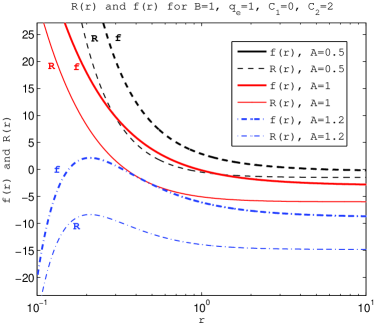
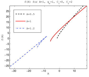
Figure 1: In the left panel we plot $R(r)$ and $f(r)$, while the right panel shows $f(R)$. We choose the coupling constants to be $B=1=q_{e}$ and the overall additive constant $C_{1}=0$. The sign of the constant $D$ influences the sign of $R$ and $f$ close to the center. For the choice $C_{2}=2$ it reduces to $D=2(A-1)$ and by plotting $f$ and $R$ for $A\in\{0.5,1,1.2\}$ we see the different behaviors: as soon as $D$ is positive (here $A>1$) $f(R)$ is not a uniquely defined function at large distances $r$ from the center.

III.0.2 Generalized Maxwell electrodynamics

To demonstrate the effect of nonlinear electrodynamics we consider a generalized form of the Maxwell theory described by the following structural function

$$H(P)\ =\ -\frac{P}{4\pi}\left[1+\frac{\mu}{1+\delta}(-2q_{e}^{2}P)^{\delta}\right]\,,$$ (41)

where $\mu$ and $\delta$ are the characteristic parameters of the theory. Note that this choice may physically describe strong fields, as the second term is now dominant, i.e. for $P\gg 1$. This Lagrangian possesses the correct Maxwell limit for $\delta>0$, i.e. $H\simeq-P/(4\pi)$ for $P\ll 1$. The relevant quantity $H_{P}$ is then given by

$$H_{P}\ =\ -\frac{1}{4\pi}\left[1+\mu(-2q_{e}^{2}P)^{\delta}\right]\,.$$ (42)

A particularly interesting and simple example is obtained by setting $\delta=1/4$, such that using Eq. (28), $H_{P}$ takes the form

$$H_{P}\ =\ -\frac{1}{4\pi}\left(1+\frac{\mu q_{e}}{r}\right)\,.$$ (43)

Thus, substituting Eq. (43) into Eq. (29), we finally deduce the following solution:

$$e^{2\alpha(r)} = 1+{\cal A}{\cal D}-\frac{2{\cal D}}{3r}+\frac{q_{e}^{2}(2-{\cal A}|q_{e}|\mu)}{2Br^{2}}+\frac{2|q_{e}|^{3}\mu}{5Br^{3}}$$ (44)

$$-\big{(}1+2{\cal A}{\cal D}\big{)}{\cal A}r-2C_{1}r^{2}+\left[\frac{1}{2}+\big{(}1+2{\cal A}{\cal D}\big{)}\ln\!\Big{(}B[{\cal A}+1/r]\Big{)}\right]{\cal A}^{2}r^{2}\,,$$

where now the effective mass is generalized to

$${\cal D}\ =\ \frac{{\cal A}\,q_{e}^{2}(2-{\cal A}|q_{e}|\mu)-C_{2}}{B}\,.$$ (45)

Note that $f(R)$ gravity coupled with Maxwell electromagnetism, i.e. $H_{P}=-1/(4\pi)$, follows from the above solution in the limit of $\mu=0$, which simply reduces to Eq. (34). Note that we can use the solution (44) to write $R(r)$ and $f(r)$ in parametric form, and finally, in principle, deduce the functional form $f(R)$. However, as outlined in Section III.0.1, $R(r)$ cannot be analytically inverted to find $r(R)$ and substitute into $f(r)$. In addition to this, we do not write out the explicit forms of $R(r)$ and $f(r)$ due to their lengthy character.

Setting $A=0$ and $B=1$, which is equivalent to general relativity, Eq. (44) provides a particularly interesting solution given by

$$e^{2\alpha(r)}\ =\ 1+\frac{2C_{2}}{3r}+\frac{q_{e}^{2}}{r^{2}}+\frac{2|q_{e}|^{3}\mu}{5r^{3}}-2C_{1}r^{2}\,,$$ (46)

which can also be found from Eq. (31). Note the presence of a term proportional to $1/r^{3}$, which dominates for low values of $r$. This solution tends to the Maxwell-Einstein limit setting $\mu=0$.

IV New solutions: $\alpha(r)\neq-\beta(r)$

Due to the fact that $f(R)$ gravity has more degrees of freedom compared to Einstein gravity, and also in view of Ref. Jacobson:2007tj , it is very interesting to explore the situation of $\alpha\neq-\beta$. However, without specifying a relation between $\alpha$ and $\beta$, a specific nonlinear electrodynamics model, or a specific $f(R)$ theory the equations are not closed and therefore analytically intractable. In this section we consider the specific example where the two metric fields satisfy the following relationship

$$\alpha(r)+\beta(r)\ =\ \ln(kr^{\ell})$$ (47)

where $k$ and $\ell$ are free parameters. This case is particularly interesting since it allows for regular electric fields at the center, as will be shown below.

From the first field equation (11) we find that $f_{R}(r)$ has the following form

$$f_{R}(r)\ =\ Ar^{p_{+}(\ell)}+Br^{p_{-}(\ell)}\,,$$ (48)

where $A$ and $B$ are constants of integration, and the exponents depend on the parameter $\ell$ as

$$p_{\pm}(\ell)\ =\ \frac{1}{2}\left(1+\ell\pm\sqrt{\ell\,(\ell+10)+1}\right)\,.$$ (49)

In order for $p_{\pm}(\ell)$ to be real it is required that either $\ell\geq 2\sqrt{6}-5$ or $\ell\leq-2\sqrt{6}-5$. In the limit $\ell=0$ the exponents become $p_{+}(0)=1$ and $p_{-}(0)=0$ such that $f_{R}(r)=Ar+B$ as in the case considered in the previous section. We plot $p_{\pm}$ in figure 2.

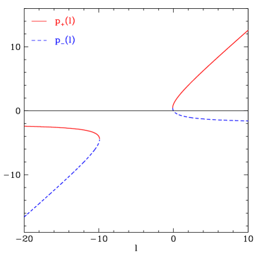
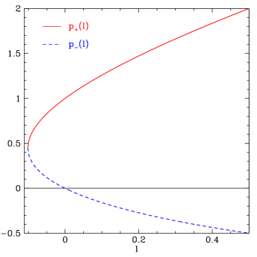
Figure 2: In the left panel we plot $p_{\pm}$, the powers of $r$ in the solution for $f_{R}(r)$, as function of the parameter $\ell$. The right panel zooms into the right branch of $p_{\pm}$. Note that $p_{-}$ vanishes for $\ell=0$, is positive for negative $\ell$ and vice versa, while $p_{-}\rightarrow-2$ for large $\ell$. This behavior makes the solution $f_{R}=Br^{p_{-}}$ particularly interesting.

The electric field now reads

$$E(r)\ =\ q_{e}kr^{\ell-2}\,H_{P}(r)\,.$$ (50)

An interesting case is $\ell=2$ where the electric field is constant in the Maxwell limit, $H_{P}=-1/(4\pi)$.

Let us consider the case $A=0$ where $f_{R}(r)$ is a simple power law which has a well defined Einstein limit for $\ell=0$ and $B=1$. For this specific case the second field equation (29) can in principle be solved for any general structural function $H_{P}(r)$. We define the constant $K=\kappa q_{e}^{2}k^{2}/B$ and solve equation (29) for $\ell\neq 1,2$, which provides the following solution

$$e^{2\alpha}\ =\ \frac{k^{2}\,r^{2\ell}}{(\ell-1)(p_{+}-2\ell-2)}+\frac{2\,r^{2}}{p_{+}-4}\left[\Big{(}C_{1}+K\int\bar{r}^{p_{+}+\ell-6}H_{P}(\bar{r})d\bar{r}\Big{)}-r^{p_{+}-4}\Big{(}C_{2}+K\int\bar{r}^{\ell-2}H_{P}(\bar{r})d\bar{r}\Big{)}\right]\,,$$ (51)

while the special cases $\ell=1,2$ have to be solved separately. For $\ell=1$, the solution is

$$e^{2\alpha}\ =\ \frac{\left(6\ln(r)-\sqrt{3}-3\right)k^{2}\,r^{2}}{3(\sqrt{3}-3)}+\frac{2\,r^{2}}{3(\sqrt{3}-3)}\left[\Big{(}C_{1}+K\int\bar{r}^{\sqrt{3}-4}H_{P}(\bar{r})d\bar{r}\Big{)}-r^{\sqrt{3}-3}\Big{(}C_{2}+K\int\frac{H_{P}(\bar{r})}{\bar{r}}d\bar{r}\Big{)}\right]\,,$$ (52)

and for $\ell=2$, we find

$$e^{2\alpha}\ =\ -\frac{1}{2}k^{2}\,r^{4}+2\,r^{2}\left[\Big{(}C_{1}+K\int\ln(\bar{r})H_{P}(\bar{r})d\bar{r}\Big{)}-\ln(r)\Big{(}C_{2}+K\int H_{P}(\bar{r})d\bar{r}\Big{)}\right]\,.$$ (53)

In all cases, the solution is not conformally flat due to the first term.

An interesting case is $f(R)$ gravity coupled to Maxwell electrodynamics where $H_{P}=-1/(4\pi)$. The electric field for this case is given by

$$E(r)\ =\ -\frac{q_{e}k}{4\pi}r^{\ell-2}$$ (54)

where for $\ell=0$, the classical Coulomb field is recovered. For $\ell<2$ it diverges at the center. Interestingly the electric field is constant for $\ell=2$, as mentioned before. For $\ell>2$ the electric field vanishes at the center and diverges at spatial infinity.

The metric field is then given in the three cases as:

$$\ell\neq 1,2\ : e^{2\alpha}\ =\ \frac{k^{2}\,r^{2\ell}}{(\ell-1)(p_{+}-2\ell-2)}+\frac{K\,r^{p_{+}+\ell-3}}{2\pi(\ell-1)(p_{+}+\ell-5)}+\frac{2\left(C_{1}\,r^{2}+C_{2}\,r^{p_{+}-2}\right)}{p_{+}-4}\,,$$ (55)

$$\ell=1\ : e^{2\alpha}\ =\ \frac{3-\sqrt{3}}{3(2-\sqrt{3})}\left\{-C_{1}\,r^{2}+C_{2}\,r^{\sqrt{3}-1}-\frac{K}{4\pi}\left[\ln(r)+(3-\sqrt{3})^{-1}\right]r^{\sqrt{3}-1}\right\}\,,$$ (56)

$$\ell=2\ : e^{2\alpha}\ =\ -\frac{1}{2}k^{2}\,r^{4}+\frac{K}{2\pi}\,r^{3}+2\,r^{2}\left[C_{1}-C_{2}\ln(r)\right]\,.$$ (57)

In the first case, the exponents of $r$ are positive in all terms for $\ell\geq\ell_{\rm crit}$, where $\ell_{\rm crit}=(5-\sqrt{13})/2\simeq 0.7$. See the left panel of figure 3 for a comparison of the different exponents. At $\ell=1$ and $\ell=2$ the hierarchy of the terms change which explains why these are special cases.

A solution is regular at the origin if the function and all its derivatives are finite at $r=0$. We verify that the solutions (56) and (57) are not regular at the origin, although they vanish for $r=0$. In case of solution (55) we only consider $2<\ell\in\mathbb{N}$ for which the electric field is regular at the origin, cf. Eq. (54). For its derivatives to be finite at the origin the following exponents of $r$

$$n_{1}\ = p_{+}+\ell-3 =\ \frac{1}{2}\left[3\ell-5+\sqrt{\ell\left(\ell+10\right)+1}\right]\,,$$ (58)

$$n_{2}\ = p_{+}-2 =\ \frac{1}{2}\left[\ell-3+\sqrt{\ell\left(\ell+10\right)+1}\right]$$ (59)

must be natural numbers, i.e. $n_{1},n_{2}\in\mathbb{N}$.

The metric function $g_{rr}$ must also be regular at the origin. Using $\alpha(r)+\beta(r)\ =\ \ln(kr^{\ell})$, we have

$$e^{2\beta}\ =\ \frac{k^{2}}{\overline{C}_{1}+\overline{C}_{2}r^{p_{+}-l-3}+\overline{C}_{3}\left(C_{1}r^{2(1-l)}+C_{2}r^{p_{+}-2-2l}\right)}\,,$$ (60)

with the constants

$$\overline{C}_{1}\ =\ \frac{k^{2}}{(\ell-1)(p_{+}-2\ell-2)}\,,\qquad\overline{C}_{2}\ =\ \frac{K}{2\pi(\ell-1)(p_{+}+\ell-5)}\,,\qquad\overline{C}_{3}\ =\ \frac{2}{p_{+}-4}$$ (61)

We have considered that $l>2$, so that we have to impose $C_{1}=0$ to have regularity at the origin. Furthermore the metric function $e^{2\beta}$ and its derivatives need to exist at the origin which means the following exponents of $r$ must be natural numbers

$$m_{1}\ = p_{+}-\ell-3 =\ \frac{1}{2}\left[-\ell-5+\sqrt{\ell\left(\ell+10\right)+1}\right]\,,$$ (62)

$$m_{2}\ = p_{+}-2(\ell+1) =\ \frac{1}{2}\left[-3(\ell+1)+\sqrt{\ell\left(\ell+10\right)+1}\right]\,.$$ (63)

However, it turns out that $m_{1}$ and $m_{2}$ are both negative for all $\ell\in\mathbb{N}$ which contradicts the imposition that $m_{1}$ and $m_{2}$ be natural numbers. Thus, we conclude that the solution (55) is not regular at the origin.

It is evident that for $\ell=1$ and $\ell=2$ the metric field goes to negative infinity for large $r>r_{0}$ and thus has to be matched to an external vacuum solution at a junction interface at $r<r_{0}$. This behavior is independent of the signs of the constants of integration $C_{1}$ and $C_{2}$. However, for the solution to be positive for small $r$, we find $C_{2}\geq 0$. In the case of $\ell>2$ we find the same behavior of the metric field and the same constraint on $C_{2}$. For $\ell_{\rm crit}\leq\ell<1$ we find positive solutions for all $r$ if $C_{2}\leq 0$ and $C_{1}\geq 0$. If $C_{1}<0$ the solution is negative for small $r>0$, if $C_{2}>0$ it tends to negative infinity for large $r$. See right panel of figure 3.

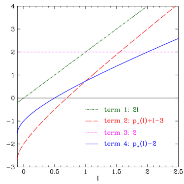
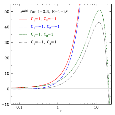
Figure 3: In the left panel the exponents of $r$ in the four terms of $e^{2\alpha(r)}$ for $\ell\neq 1,2$ are plotted. For $\ell\geq\ell_{\rm crit}\simeq 0.7$ the exponents of $r$ are positive in all terms. Negative $\ell$ lead to solutions divergent at the center. At $\ell=1$ and $\ell=2$ the hierarchy of the terms change which explains why these are special cases. The right panel shows $e^{2\alpha(r)}$ for $\ell=0.8$ for four different combinations of signs of the integration constants, while for simplicity and transparency we set $K=1=k^{2}$ throughout the analysis.

We also emphasize that through $R(r)$ and $f(r)$ (not written out explicitly due to their extremely lengthy nature) expressed in parametric form, the functional form $f(R)$ may in principle be deduced. However, as outlined in Section III.0.1, $R(r)$ cannot be analytically inverted to find $r(R)$ and substitute into $f(r)$.

V Alternative approaches

V.1 Constant curvature

An interesting alternative is to consider the specific case of constant curvature $R(r)=R_{0}$. Note that in this case $f_{R}$ is independent of $r$, and for simplicity one may set $f_{R}(r)=B$. Thus, one verifies that Eq. (11) yields $\alpha(r)=-\beta(r)$, so that the curvature scalar is given by

$$R\ =\ -\frac{2e^{2\alpha(r)}}{r^{2}}\left[4r\alpha^{\prime}+r^{2}\alpha^{\prime\prime}+2r^{2}(\alpha^{\prime})^{2}-e^{-2\alpha}+1\right]\,.$$ (64)

For constant curvature, $R(r)=R_{0}$, this yields the following solution for $\alpha(r)$

$$e^{2\alpha(r)}\ =\ 1-\frac{2C_{1}}{r}+\frac{2C_{2}}{r^{2}}-\frac{R_{0}}{12}r^{2}\,.$$ (65)

Substituting the metric field into Eq. (29), one deduces $H_{P}$, given by

$$H_{P}(r)\ =\ -\frac{C_{2}B}{2\pi q_{e}^{2}}\,.$$ (66)

which reduces to the Maxwell type, i.e. $H_{P}=-1/(4\pi)$, by setting the constant of integration $C_{2}=q_{e}^{2}/(2B)$.

For this case, i.e. constant curvature, and taking into account that the Maxwell limit implies $T=0$ (see Section II.1), the trace equation (9) imposes the following algebraic relationship

$$f_{R}R-2f\ =\ 0\,,$$ (67)

so that the form of $f(R)$ needs to obey this algebraic identity. Thus the metric given by Eq. (65) is an exact solution for the class of solutions $f(R)$, in the Maxwell limit, that satisfy $f_{R}(R_{0})R_{0}-2f(R_{0})=0$. For instance, considering the case of $f(R)=R-\mu^{4}/R$, and using the above trace equation yields $R_{0}=\pm\sqrt{\mu^{2}}$. The case of $f(R)=R+\gamma^{2}R^{2}$, provides $R_{0}=0$.

V.2 Specific gravity theory: $f(R)=R+\bar{\gamma}^{2}R^{2}$

Another alternative approach is to consider specific choices for the form of $f(R)$. Consider the specific case of $f(R)=R+\bar{\gamma}^{2}R^{2}$, which for $\alpha(r)=-\beta(r)$ implies that $Ar+B=1+\gamma^{2}R$, with $\gamma^{2}=2\bar{\gamma}^{2}$. Substituting the value for $R(r)$, provides the following solution:

$$e^{2\alpha(r)}\ =\ 1-\frac{2C_{2}}{r}+\frac{2C_{1}}{r^{2}}+\frac{(1-B)}{12\gamma^{2}}r^{2}-\frac{A}{20\gamma^{2}}r^{3}\,.$$ (68)

Note that this solution is consistent with Eq. (11), i.e. $f_{R}^{\prime\prime}(r)=\gamma^{2}R^{\prime\prime}(r)=0$.

Now, substituting this solution in Eq. (12), and finally using the relationship $P=-q_{e}^{2}/(2r^{4})$, we reconstruct the following nonlinear electrodynamic structural function

$$H(P) = -\frac{C_{1}B}{2\pi q_{e}^{2}}P+\frac{A}{2\pi q_{e}^{2}}\Bigg{[}3C_{2}|q_{e}|(-2P)^{\frac{1}{2}}-2|q_{e}|^{\frac{3}{2}}(-2P)^{\frac{1}{4}}+\frac{B|q_{e}|^{\frac{5}{2}}}{5\gamma^{2}}(-2P)^{-\frac{1}{4}}+\frac{A|q_{e}|^{\frac{3}{2}}}{8\gamma^{2}}(-2P)^{-\frac{1}{2}}\Bigg{]}\,.$$ (69)

Note that for $A=0$ and $C_{1}=q_{e}^{2}/(2B)$ it reduces to the Maxwell type, i.e. $H=-P/(4\pi)$. However, for $A\neq 0$ this structural function does not tend to the Maxwell limit for $P\ll 1$. Therefore it is not a viable nonlinear electrodynamic theory. This specific case illustrates the difficulty in finding viable nonlinear electrodynamic theories, i.e. with the correct Maxwell limit, by explicitly providing a form for $f(R)$.

VI Conclusion

The issue of exact static and spherically symmetric solutions in $f(R)$ modified theories of gravity is an important theme, mainly due to the analysis of weak field solar system constraints, and the generalization of exact general relativistic solutions to $f(R)$ gravity. In this work we have analyzed exact solutions of static and spherically symmetric space-times in $f(R)$ modified theories of gravity coupled to nonlinear electrodynamics. Firstly, the metric fields were restricted to one degree of freedom, by considering the specific case of $g_{tt}=-g_{rr}^{-1}$. Using the dual $P$ formalism of nonlinear electrodynamics, an exact general solution was found in terms of the structural function $H_{P}$. In particular, exact solutions to the gravitational field equations were found, confirming previous results and new pure electric field solutions were deduced. Secondly, by allowing two degrees of freedom for the metric fields, and motivated by the existence of regular electric fields at the center, new solutions were found. Finally, we have also briefly considered alternative approaches by analyzing the specific case of constant curvature and secondly, by considering a specific form for $f(R)$.

- (1) S. Perlmutter et al., Astrophys. J. 517, 565 (1999); A. G. Riess et al., Astron. J. 116, 1009 (1998); A. G. Riess et al., Astrophys. J. 607, 665 (2004) A. Grant et al, Astrophys. J. 560 49-71 (2001); S. Perlmutter, M. S. Turner and M. White, Phys. Rev. Lett. 83 670-673 (1999); C. L. Bennett et al, Astrophys. J. Suppl. 148 1 (2003); G. Hinshaw et al, Astrophys. J. Suppl. 148, 135 (2003).
- (2) A. A. Starobinsky, Phys. Lett. B 91, 99 (1980).
- (3) S. M. Carroll, V. Duvvuri, M. Trodden and M. S. Turner, Phys. Rev. D 70, 043528 (2004).
- (4) S. Fay, R. Tavakol and S. Tsujikawa, Phys. Rev. D 75, (2007) 063509.
- (5) S. Nojiri and S. D. Odintsov, Phys. Rev. D 74 (2006) 086005; S. Nojiri and S. D. Odintsov, J. Phys. Conf. Ser. 66, 012005 (2007); S. Capozziello, S. Nojiri, S. D. Odintsov and A. Troisi, Phys. Lett. B 639 (2006) 135; S. Nojiri and S. D. Odintsov, arXiv:0804.3519 [hep-th].
- (6) G. Cognola, E. Elizalde, S. Nojiri, S. D. Odintsov and S. Zerbini, Phys. Rev. D 73, 084007 (2006)
- (7) S. Capozziello, V. F. Cardone and A. Troisi, JCAP 0608, 001 (2006); S. Capozziello, V. F. Cardone and A. Troisi, Mon. Not. R. Astron. Soc. 375, 1423 (2007); A. Borowiec, W. Godlowski and M. Szydlowski, Int. J. Geom. Meth. Mod. Phys. 4 (2007) 183; C. F. Martins and P. Salucci, Mon. Not. Roy. Astron. Soc. 381, 1103 (2007); C. G. Boehmer, T. Harko and F. S. N. Lobo, Astropart. Phys. 29, 386-392 (2008); C. G. Boehmer, T. Harko and F. S. N. Lobo, JCAP 0803, 024 (2008); F. S. N. Lobo, arXiv:0807.1640 [gr-qc].
- (8) S. Nojiri and S. D. Odintsov, Phys. Lett. B 599 (2004) 137; G. Allemandi, A. Borowiec, M. Francaviglia and S. D. Odintsov, Phys. Rev. D 72 (2005) 063505; T. Koivisto, Class. Quant. Grav. 23, (2006) 4289; O. Bertolami, C. G. Böhmer, T. Harko and F. S. N. Lobo, Phys. Rev. D 75 (2007) 104016; O. Bertolami and J. Páramos, Phys. Rev. D 77, 084018 (2008); V. Faraoni, Phys. Rev. D 76, 127501 (2007); O. Bertolami and J. Páramos, arXiv:0805.1241 [gr-qc]; T. P. Sotiriou, arXiv:0805.1160 [gr-qc]; T. P. Sotiriou and V. Faraoni, arXiv:0805.1249 [gr-qc]; O. Bertolami, F. S. N. Lobo and J. Páramos, Phys. Rev. D 78, 064036 (2008).
- (9) G. J. Olmo, Phys. Rev. Lett. 98, (2007) 061101.
- (10) M. Amarzguioui, O. Elgaroy, D. F. Mota and T. Multamaki, Astron. Astrophys. 454 (2006) 707; L. Amendola, D. Polarski and S. Tsujikawa, Phys. Rev. Lett. 98, (2007) 131302; L. Amendola, R. Gannouji, D. Polarski and S. Tsujikawa, Phys. Rev. D 75, (2007) 083504; T. Koivisto, Phys. Rev. D 76, 043527 (2007); A. A. Starobinsky, JETP Lett. 86, 157 (2007).
- (11) W. Hu and I. Sawicki, Phys. Rev. D 76, 064004 (2007).
- (12) L. M. Sokolowski, Class. Quant. Grav. 24 3391-3411 (2007).
- (13) T. Chiba, Phys. Lett. B 575, (2003) 1; A. L. Erickcek, T. L. Smith and M. Kamionkowski, Phys. Rev. D 74, (2006) 121501(R); T. Chiba, T. L. Smith and A. L. Erickcek, Phys. Rev. D 75, 124014 (2007); G. J. Olmo, Phys. Rev. D 75 (2007) 023511.
- (14) S. Nojiri and S. D. Odintsov, Phys. Rev. D 68 (2003) 123512; V. Faraoni, Phys. Rev. D 74 (2006) 023529; T. Faulkner, M. Tegmark, E. F. Bunn and Y. Mao, Phys. Rev. D 76, 063505 (2007).
- (15) I. Sawicki and W. Hu, Phys. Rev. D 75, 127502 (2007).
- (16) L. Amendola and S. Tsujikawa, Phys. Lett. B 660, 125 (2008).
- (17) V. Faraoni, Phys. Rev. D 74, (2006) 104017; S. Carloni, P. K. S. Dunsby, S. Capozziello and A. Troisi, Class. Quant. Grav. 22 (2005) 4839; J. A. Leach, S. Carloni and P. K. S. Dunsby, Class. Quant. Grav. 23 (2006) 4915; S. Carloni, A. Troisi and P. K. S. Dunsby, arXiv:0706.0452 [gr-qc].
- (18) C. G. Böhmer, L. Hollenstein and F. S. N. Lobo, Phys. Rev. D 76, 084005 (2007); R. Goswami, N. Goheer and P. K. S. Dunsby, arXiv:0804.3528 [gr-qc].
- (19) G. Cognola, E. Elizalde, S. Nojiri, S. D. Odintsov and S. Zerbini, JCAP 0502 (2005) 010; V. Faraoni, Phys. Rev. D 72, (2005) 061501(R); V. Faraoni, S. Nadeau, Phys. Rev. D 72, (2005) 124005; V. Faraoni, Phys. Rev. D 75, (2007) 067302; G. Cognola, M. Gastaldi and S. Zerbini, Int. J. Theor. Phys. 47, 898 (2008).
- (20) S. Nojiri and S. D. Odintsov, Int. J. Geom. Meth. Mod. Phys. 4 (2007) 115.
- (21) T. Koivisto and H. Kurki-Suonio, Class. Quant. Grav. 23, (2006) 2355; R. Bean, D. Bernat, L. Pogosian, A. Silvestri and M. Trodden, Phys. Rev. D 75, (2007) 064020.
- (22) S. Tsujikawa, Phys. Rev. D 76, 023514 (2007).
- (23) K. Uddin, J. E. Lidsey and R. Tavakol, Class. Quant. Grav. 24, 3951 (2007).
- (24) D. Bazeia, B. Carneiro da Cunha, R. Menezes and A. Y. Petrov, Phys. Lett. B 649 (2007) 445.
- (25) T. Clifton and J. D. Barrow, Phys. Rev. D 72, 103005 (2005).
- (26) T. Multamaki and I. Vilja, Phys. Rev. D 76, 064021 (2007); K. Kainulainen, J. Piilonen, V. Reijonen and D. Sunhede, Phys. Rev. D 76, 024020 (2007); S. Capozziello, A. Stabile and A. Troisi, Class. Quant. Grav. 24, (2007) 2153; M. D. Seifert, Phys. Rev. D 76, 064002 (2007).
- (27) T. Multamaki and I. Vilja, Phys. Rev. D 74, 064022 (2006).
- (28) T. Multamaki and I. Vilja, Phys. Rev. D 76, 064021 (2007).
- (29) S. Capozziello, A. Stabile and A. Troisi, Class. Quant. Grav. 24, 2153 (2007).
- (30) S. Capozziello, A. Stabile and A. Troisi, Phys. Rev. D 76, 104019 (2007).
- (31) K. Kainulainen, J. Piilonen, V. Reijonen and D. Sunhede, Phys. Rev. D 76, 024020 (2007).
- (32) K. Henttunen, T. Multamaki and I. Vilja, Phys. Rev. D 77, 024040 (2008).
- (33) T. Multamaki and I. Vilja, Phys. Lett. B 659, 843 (2008).
- (34) I. Dymnikova, Class. Quant. Grav. 21, 4417 (2004).
- (35) P. D. Mannheim and D. Kazanas, Astroph. Journ. 342, 635 (1989); D. Kazanas and P. D. Mannheim, Astroph. Journ. Supp. Series 76, 421 (1991).
- (36) K. Bamba and S. D. Odintsov, JCAP 0804, 024 (2008).
- (37) M. Born, Proc. Roy. Soc. Lond. A143, 410 (1934); M. Born and L. Infeld, Proc. Roy. Soc. A144, 425 (1934).
- (38) J. F. Plebański, “Lectures on non-linear electrodynamics,” monograph of the Niels Bohr Institute Nordita, Copenhagen (1968).
- (39) N. Seiberg and E. Witten, JHEP 9909, 032 (1999).
- (40) R. Garcia-Salcedo and N. Breton, Int. J. Mod. Phys. A 15, 4341 (2000); R. Garcia-Salcedo and N. Breton, Class. Quant. Grav. 20, 5425 (2003); R. Garcia-Salcedo and N. Breton, Class. Quant. Grav. 22, 4783 (2005); V. V. Dyadichev, D. V. Gal’tsov, A. G. Zorin and M. Yu. Zotov, Phys. Rev. D 65, 084007 (2002); D. N. Vollick, Gen. Rel. Grav. 35, 1511-1516 (2003).
- (41) M. Novello, S. E. Perez Bergliaffa and J. Salim, Phys. Rev. D 69, 127301 (2004).
- (42) E. Ayón-Beato and A. García, Phys. Rev. Lett. 80, 5056-5059 (1998).
- (43) E. Ayón-Beato and A. García, Phys. Lett. B 464, 25 (1999); E. Ayón-Beato and A. García, Gen. Rel. Grav. 31, 629-633 (1999).
- (44) K. A. Bronnikov, Phys. Rev. D 63, 044005 (2001).
- (45) I. Dymnikova, Class. Quant. Grav. 21, 4417-4429 (2004).
- (46) A. V. B. Arellano and F. S. N. Lobo, Class. Quant. Grav. 23, 5811 (2006); A. V. B. Arellano and F. S. N. Lobo, Class. Quant. Grav. 23, 7229 (2006); A. V. B. Arellano, N. Breton and R. Garcia-Salcedo, arXiv:0804.3944 [gr-qc].
- (47) F. S. N. Lobo and A. V. B. Arellano, Class. Quant. Grav. 24, 1069 (2007).
- (48) T. Jacobson, Class. Quant. Grav. 24, 5717 (2007).