Nemirovski’s Inequalities Revisited

1 Introduction.

Our starting point is the following well known theorem from probability: Let $X_{1},\ldots,X_{n}$ be (stochastically) independent random variables with finite second moments, and let $S_{n}=\sum_{i=1}^{n}X_{i}$. Then

$$\mathop{\rm Var}\nolimits(S_{n})=\sum_{i=1}^{n}\mathop{\rm Var}\nolimits(X_{i}).$$ (1)

If we suppose that each $X_{i}$ has mean zero, $\mathop{\rm I\!E}\nolimits X_{i}=0$, then (1) becomes

$$\mathop{\rm I\!E}\nolimits S_{n}^{2}=\sum_{i=1}^{n}\mathop{\rm I\!E}\nolimits X_{i}^{2}.$$ (2)

This equality generalizes easily to vectors in a Hilbert space $\mathbb{H}$ with inner product $\langle\cdot,\cdot\rangle$: If the $X_{i}$’s are independent with values in $\mathbb{H}$ such that $\mathop{\rm I\!E}\nolimits X_{i}=0$ and $\mathop{\rm I\!E}\nolimits\|X_{i}\|^{2}<\infty$, then $\|S_{n}\|^{2}=\langle S_{n},S_{n}\rangle=\sum_{i,j=1}^{n}\langle X_{i},X_{j}\rangle$, and since $\mathop{\rm I\!E}\nolimits\langle X_{i},X_{j}\rangle=0$ for $i\not=j$ by independence,

$$\mathop{\rm I\!E}\nolimits\|S_{n}\|^{2}=\sum_{i,j=1}^{n}\mathop{\rm I\!E}\nolimits\langle X_{i},X_{j}\rangle=\sum_{i=1}^{n}\mathop{\rm I\!E}\nolimits\|X_{i}\|^{2}.$$ (3)

What happens if the $X_{i}$’s take values in a (real) Banach space $(\mathbb{B},\|\cdot\|)$? In such cases, in particular when the square of the norm $\|\cdot\|$ is not given by an inner product, we are aiming at inequalities of the following type: Let $X_{1}$, $X_{2}$, …, $X_{n}$ be independent random vectors with values in $(\mathbb{B},\|\cdot\|)$ with $\mathop{\rm I\!E}\nolimits X_{i}=0$ and $\mathop{\rm I\!E}\nolimits\|X_{i}\|^{2}<\infty$. With $S_{n}:=\sum_{i=1}^{n}X_{i}$ we want to show that

$$\mathop{\rm I\!E}\nolimits\|S_{n}\|^{2}\ \leq\ K\sum_{i=1}^{n}\mathop{\rm I\!E}\nolimits\|X_{i}\|^{2}$$ (4)

for some constant $K$ depending only on $(\mathbb{B},\|\cdot\|)$.

For statistical applications, the case $(\mathbb{B},\|\cdot\|)=\ell_{r}^{d}:=(\mathbb{R}^{d},\|\cdot\|_{r})$ for some $r\in[1,\infty]$ is of particular interest. Here the $r$-norm of a vector $x\in\mathbb{R}^{d}$ is defined as

$$\|x\|_{r}\ :=\begin{cases}\displaystyle\Bigl{(}\sum_{j=1}^{d}|x_{j}|^{r}\Bigr{)}^{1/r}&\text{if}\ 1\leq r<\infty,\\ \displaystyle\max_{1\leq j\leq d}\,|x_{j}|&\text{if}\ r=\infty.\end{cases}$$ (5)

An obvious question is how the exponent $r$ and the dimension $d$ enter an inequality of type (4). The influence of the dimension $d$ is crucial, since current statistical research often involves small or moderate “sample size” $n$ (the number of independent units), say on the order of $10^{2}$ or $10^{4}$, while the number $d$ of items measured for each independent unit is large, say on the order of $10^{6}$ or $10^{7}$. The following two examples for the random vectors $X_{i}$ provide lower bounds for the constant $K$ in (4):

Example 1.1.

(A lower bound in $\ell_{r}^{d}$)   Let $b_{1},b_{2},\ldots,b_{d}$ denote the standard basis of $\mathbb{R}^{d}$, and let $\epsilon_{1},\epsilon_{2},\ldots,\epsilon_{d}$ be independent Rademacher variables, i.e. random variables taking the values $+1$ and $-1$ each with probability $1/2$. Define $X_{i}:=\epsilon_{i}b_{i}$ for $1\leq i\leq n:=d$. Then $\mathop{\rm I\!E}\nolimits X_{i}=0$, $\|X_{i}\|_{r}^{2}=1$, and $\|S_{n}\|_{r}^{2}=d^{2/r}=d^{2/r-1}\sum_{i=1}^{n}\|X_{i}\|_{r}^{2}$. Thus any candidate for $K$ in (4) has to satisfy $K\geq d^{2/r-1}$.

Example 1.2.

(A lower bound in $\ell_{\infty}^{d}$)   Let $X_{1},X_{2},X_{3},\ldots$ be independent random vectors, uniformly distributed on $\{-1,1\}^{d}$ each. Then $\mathop{\rm I\!E}\nolimits X_{i}=0$ and $\|X_{i}\|_{\infty}=1$. On the other hand, according to the Central Limit Theorem, $n^{-1/2}S_{n}$ converges in distribution as $n\to\infty$ to a random vector $Z=(Z_{j})_{j=1}^{d}$ with independent, standard Gaussian components, $Z_{j}\sim N(0,1)$. Hence

$$\sup_{n\geq 1}\frac{\mathop{\rm I\!E}\nolimits\|S_{n}\|_{\infty}^{2}}{\sum_{i=1}^{n}\mathop{\rm I\!E}\nolimits\|X_{i}\|_{\infty}^{2}}=\sup_{n\geq 1}\mathop{\rm I\!E}\nolimits\|n^{-1/2}S_{n}\|_{\infty}^{2}\ \geq\ \mathop{\rm I\!E}\nolimits\|Z\|_{\infty}^{2}=\mathop{\rm I\!E}\nolimits\max_{1\leq j\leq d}Z_{j}^{2}.$$

But it is well-known that $\max_{1\leq j\leq d}|Z_{j}|=\sqrt{2\log d}+o_{p}(1)$ as $d\to\infty$. Thus candidates $K(d)$ for the constant in (4) have to satisfy

$$\liminf_{d\to\infty}\frac{K(d)}{2\log d}\ \geq\ 1.$$

At least three different methods have been developed to prove inequalities of the form given by (4). The three approaches known to us are:

(a) deterministic inequalities for norms;
(b) probabilistic methods for Banach spaces;
(c) empirical process methods.

Approach (a) was used by Nemirovski [14] to show that in the space $\ell_{r}^{d}$ with $d\geq 2$, inequality (4) holds with $K=C\min(r,\log(d))$ for some universal (but unspecified) constant $C$. In view of Example 1.2, this constant has the correct order of magnitude if $r=\infty$. For statistical applications see Greenshtein and Ritov [7]. Approach (b) uses special moment inequalities from probability theory on Banach spaces which involve nonrandom vectors in $\mathbb{B}$ and Rademacher variables as introduced in Example 1.1. Empirical process theory (approach (c)) in general deals with sums of independent random elements in infinite-dimensional Banach spaces. By means of chaining arguments, metric entropies and approximation arguments, “maximal inequalities” for such random sums are built from basic inequalities for sums of independent random variables or finite-dime nsional random vectors, in particular, “exponential inequalities”; see e.g. Dudley [4], van der Vaart and Wellner [26], Pollard [21], de la Pena and Giné [3], or van de Geer [25].

Our main goal in this paper is to compare the inequalities resulting from these different approaches and to refine or improve the constants $K$ obtainable by each method. The remainder of this paper is organized as follows: In Section 2 we review several deterministic inequalities for norms and, in particular, key arguments of Nemirovski [14]. Our exposition includes explicit and improved constants. While finishing the present paper we became aware of yet unpublished work of [15] and [12] who also improved some inequalities of [14]. Rio [22] uses similar methods in a different context. In Section 3 we present inequalities of type (4) which follow from type and co-type inequalities developed in probability theory on Banach spaces. In addition, we provide and utilize a new type inequality for the normed space $\ell_{\infty}^{d}$. To do so we utilize, among other tools, exponential inequalities of Hoeffding [9] and Pinelis [17]. In Section 4 we follow approach (c) and treat $\ell_{\infty}^{d}$ by means of a truncation argument and Bernstein’s exponential inequality. Finally, in Section 5 we compare the inequalities resulting from these three approaches. In that section we relax the assumption that $\mathop{\rm I\!E}\nolimits X_{i}=0$ for a more thorough understanding of the differences between the three approaches. Most proofs are deferred to Section 6.

2 Nemirovski’s approach: Deterministic inequalities for
norms.

In this section we review and refine inequalities of type (4) based on deterministic inequalities for norms. The considerations for $(\mathbb{B},\|\cdot\|)=\ell_{r}^{d}$ follow closely the arguments of [14].

2.1 Some inequalities for $\mathbb{R}^{d}$ and the norms $\|\cdot\|_{r}$

Throughout this subsection let $\mathbb{B}=\mathbb{R}^{d}$, equipped with one of the norms $\|\cdot\|_{r}$ defined in (5). For $x\in\mathbb{R}^{d}$ we think of $x$ as a column vector and write $x^{\top}$ for the corresponding row vector. Thus $xx^{\top}$ is a $d\times d$ matrix with entries $x_{i}x_{j}$ for $i,j\in\{1,\ldots,d\}$.

A first solution.

Recall that for any $x\in\mathbb{R}^{d}$,

$$\|x\|_{r}\ \leq\ \|x\|_{q}\ \leq\ d^{1/q-1/r}\|x\|_{r}\quad\text{for}\ 1\leq q<r\leq\infty.$$ (6)

Moreover, as mentioned before,

$$\mathop{\rm I\!E}\nolimits\|S_{n}\|_{2}^{2}\ =\ \sum_{i=1}^{n}\mathop{\rm I\!E}\nolimits\|X_{i}\|_{2}^{2}.$$

Thus for $1\leq q<2$,

$$\mathop{\rm I\!E}\nolimits\|S_{n}\|_{q}^{2}\ \leq\ (d^{1/q-1/2})^{2}\mathop{\rm I\!E}\nolimits\|S_{n}\|_{2}^{2}\ =\ d^{2/q-1}\sum_{i=1}^{n}\mathop{\rm I\!E}\nolimits\|X_{i}\|_{2}^{2}\ \leq\ d^{2/q-1}\sum_{i=1}^{n}\mathop{\rm I\!E}\nolimits\|X_{i}\|_{q}^{2},$$

whereas for $2<r\leq\infty$,

$$\mathop{\rm I\!E}\nolimits\|S_{n}\|_{r}^{2}\ \leq\ \mathop{\rm I\!E}\nolimits\|S_{n}\|_{2}^{2}\ =\ \sum_{i=1}^{n}\mathop{\rm I\!E}\nolimits\|X_{i}\|_{2}^{2}\ \leq\ d^{1-2/r}\sum_{i=1}^{n}\mathop{\rm I\!E}\nolimits\|X_{i}\|_{r}^{2}.$$

Thus we may conclude that (4) holds with

$$K=\widetilde{K}(d,r)\ :=\ \begin{cases}d^{2/r-1}&\text{if}\ 1\leq r\leq 2,\\ d^{1-2/r}&\text{if}\ 2\leq r\leq\infty.\end{cases}$$

Example 1.1 shows that this constant $\widetilde{K}(d,r)$ is indeed optimal for $1\leq r\leq 2$.

A refinement for $r>2$.

In what follows we shall replace $\widetilde{K}(d,r)=d^{1-2/r}$ with substantially smaller constants. The main ingredient is the following result:

Lemma 2.1.

For arbitrary fixed $r\in[2,\infty)$ and $x\in\mathbb{R}^{d}\setminus\{0\}$ let

$$h(x)\ :=\ 2\|x\|_{r}^{2-r}\bigl{(}|x_{i}|^{r-2}x_{i}\bigr{)}_{i=1}^{d}$$

while $h(0):=0$. Then for arbitrary $x,y\in\mathbb{R}^{d}$,

$$\|x\|_{r}^{2}+h(x)^{\top}y\ \leq\ \|x+y\|_{r}^{2}\ \leq\ \|x\|_{r}^{2}+h(x)^{\top}y+(r-1)\|y\|_{r}^{2}.$$

[16] and [14] stated Lemma 2.1 with the factor $r-1$ on the right side replaced with $Cr$ for some (absolute) constant $C>1$. Lemma 2.1, which is a special case of the more general Lemma 2.4 in the next subsection, may be applied to the partial sums $S_{0}:=0$ and $S_{k}:=\sum_{i=1}^{k}X_{i}$, $1\leq k\leq n$, to show that for $2\leq r<\infty$,

$$\mathop{\rm I\!E}\nolimits\|S_{k}\|_{r}^{2} \leq \mathop{\rm I\!E}\nolimits\bigl{(}\|S_{k-1}\|_{r}^{2}+h(S_{k-1})^{\top}X_{k}+(r-1)\|X_{k}\|_{r}^{2}\bigr{)}$$

$$= \mathop{\rm I\!E}\nolimits\|S_{k-1}\|_{r}^{2}+\mathop{\rm I\!E}\nolimits h(S_{k-1})^{\top}\mathop{\rm I\!E}\nolimits X_{k}+(r-1)\mathop{\rm I\!E}\nolimits\|X_{k}\|_{r}^{2}$$

$$= \mathop{\rm I\!E}\nolimits\|S_{k-1}\|_{r}^{2}+(r-1)\mathop{\rm I\!E}\nolimits\|X_{k}\|_{r}^{2},$$

and inductively we obtain a second candidate for $K$ in (4):

$$\mathop{\rm I\!E}\nolimits\|S_{n}\|_{r}^{2}\ \leq\ (r-1)\sum_{i=1}^{n}\mathop{\rm I\!E}\nolimits\|X_{i}\|_{r}^{2}\quad\text{for}\ 2\leq r<\infty.$$

Finally, we apply (6) again: For $2\leq q\leq r\leq\infty$ with $q<\infty$,

$$\mathop{\rm I\!E}\nolimits\|S_{n}\|_{r}^{2}\ \leq\ \mathop{\rm I\!E}\nolimits\|S_{n}\|_{q}^{2}\\ \ \leq\ (q-1)\sum_{i=1}^{n}\mathop{\rm I\!E}\nolimits\|X_{i}\|_{q}^{2}\\ \ \leq\ (q-1)d^{2/q-2/r}\sum_{i=1}^{n}\mathop{\rm I\!E}\nolimits\|X_{i}\|_{r}^{2}.$$

This inequality entails our first ($q=2$) and second ($q=r<\infty$) preliminary result, and we arrive at the following refinement:

Theorem 2.2.

For arbitrary $r\in[2,\infty]$,

$$\mathop{\rm I\!E}\nolimits\|S_{n}\|_{r}^{2}\ \leq\ K_{\rm Nem}(d,r)\sum_{i=1}^{n}\mathop{\rm I\!E}\nolimits\|X_{i}\|_{r}^{2}$$

with

$$K_{\rm Nem}(d,r)\ :=\ \inf_{q\in[2,r]\cap\mathbb{R}}(q-1)d^{2/q-2/r}.$$

This constant $K_{\rm Nem}(d,r)$ satisfies the (in)equalities

$$K_{\rm Nem}(d,r)\ \left\{\begin{array}[]{ccl}=&d^{1-2/r}&\text{if}\ d\leq 7\\ \leq&r-1\\ \leq&2e\log d-e&\text{if}\ d\geq 3,\end{array}\right.$$

and

$$K_{\rm Nem}(d,\infty)\ \geq\ 2e\log d-3e.$$

Corollary 2.3.

In case of $(\mathbb{B},\|\cdot\|)=\ell_{\infty}^{d}$ with $d\geq 3$, inequality (4) holds with constant $K=2e\log d-e$. If the $X_{i}$’s are also identically distributed, then

$$\mathop{\rm I\!E}\nolimits\|n^{-1/2}S_{n}\|_{\infty}^{2}\ \leq\ (2e\log d-e)\mathop{\rm I\!E}\nolimits\|X_{1}\|_{\infty}^{2}.$$

Note that

$$\lim_{d\to\infty}\frac{K_{\rm Nem}(d,\infty)}{2\log d}\ =\ \lim_{d\to\infty}\frac{2e\log d-e}{2\log d}\ =\ e.$$

Thus Example 1.2 entails that for large dimension $d$, the constants $K_{\rm Nem}(d,\infty)$ and $2e\log d-e$ are optimal up to a factor close to $e\ \dot{=}\ 2.7183$.

2.2 Arbitrary $L_{r}$-spaces

Lemma 2.1 is a special case of a more general inequality: Let $(T,\Sigma,\mu)$ be a $\sigma$-finite measure space, and for $1\leq r<\infty$ let $L_{r}(\mu)$ be the set of all measurable functions $f:T\to\mathbb{R}$ with finite (semi-) norm

$$\|f\|_{r}\ :=\ \Bigl{(}\int|f|^{r}\,d\mu\Bigr{)}^{1/r},$$

where two such functions are viewed as equivalent if they coincide almost everywhere with respect to $\mu$. In what follows we investigate the functional

$$f\ \mapsto\ V(f):=\|f\|_{r}^{2}$$

on $L_{r}(\mu)$. Note that $(\mathbb{R}^{d},\|\cdot\|_{r})$ corresponds to $(L_{r}(\mu),\|\cdot\|_{r})$ if we take $T=\{1,2,\ldots,d\}$ equipped with counting measure $\mu$.

Note that $V(\cdot)$ is convex; thus for fixed $f,g\in L_{r}(\mu)$, the function

$$v(t)\ :=\ V(f+tg)=\|f+tg\|_{r}^{2},\qquad t\in\mathbb{R}$$

is convex with derivative

$$v^{\prime}(t)=v^{1-r/2}(t)\int 2|f+tg|^{r-2}(f+tg)g\,d\mu.$$

By convexity of $v$ it follows that

$$V(f+g)-V(f)=v(1)-v(0)\geq v^{\prime}(0)\ :=\ DV(f,g).$$

This proves the lower bound in the following lemma. We will prove the upper bound in Section 6 by computation of $v^{\prime\prime}$ and application of Hölder’s inequality.

Lemma 2.4.

Let $r\geq 2$. Then for arbitrary $f,g\in L_{r}(\mu)$,

$$DV(f,g)\ =\ \int h(f)g\,d\mu\quad\text{with}\quad h(f)\ :=\ 2\|f\|_{r}^{2-r}|f|^{r-2}f\ \in\ L_{q}(\mu),$$

where $q:=r/(r-1)$. Moreover,

$$V(f)+DV(f,g)\ \leq\ V(f+g)\ \leq\ V(f)+DV(f,g)+(r-1)V(g).$$

Remark 2.5.

The upper bound for $V(f+g)$ is sharp in the following sense: Suppose that $\mu(T)<\infty$, and let $f,g_{o}:T\to\mathbb{R}$ be measurable such that $|f|\equiv|g_{o}|\equiv 1$ and $\int fg_{o}\,d\mu=0$. Then our proof of Lemma 2.4 reveals that

$$\frac{V(f+tg_{o})-V(f)-DV(f,tg_{o})}{V(tg_{o})}\ \to\ r-1\quad\text{as}\ t\to 0.$$

Remark 2.6.

In case of $r=2$, Lemma 2.4 is well known and easily verified. Here the upper bound for $V(f+g)$ is even an equality, i.e.

$$V(f+g)\ =\ V(f)+DV(f,g)+V(g).$$

Remark 2.7.

Lemma 2.4 improves on an inequality of [16]. After writing this paper we realized Lemma 2.4 is also proved by [18]; see his (2.2) and Proposition 2.1, page 1680.

Lemma 2.4 leads directly to the following result:

Corollary 2.8.

In case of $\mathbb{B}=L_{r}(\mu)$ for $r\geq 2$, inequality (4) is satisfied with $K=r-1$.

2.3 A connection to geometrical functional analysis

For any Banach space $(\mathbb{B},\|\cdot\|)$ and Hilbert space $(\mathbb{H},\langle\cdot,\cdot\rangle,\|\cdot\|)$, their Banach-Mazur distance $D(\mathbb{B},\mathbb{H})$ is defined to be the infimum of

$$\|T\|\cdot\|T^{-1}\|$$

over all linear isomorphisms $T:\mathbb{B}\to\mathbb{H}$, where $\|T\|$ and $\|T^{-1}\|$ denote the usual operator norms

$$\|T\| := \sup\bigl{\{}\|Tx\|:x\in\mathbb{B},\|x\|\leq 1\bigr{\}},$$

$$\|T^{-1}\| := \sup\bigl{\{}\|T^{-1}y\|:y\in\mathbb{H},\|y\|\leq 1\bigr{\}}.$$

(If no such bijection exists, one defines $D(\mathbb{B},\mathbb{H}):=\infty$.) Given such a bijection $T$,

$$\mathop{\rm I\!E}\nolimits\|S_{n}\|^{2} \leq \|T^{-1}\|^{2}\mathop{\rm I\!E}\nolimits\|TS_{n}\|^{2}$$

$$= \|T^{-1}\|^{2}\sum_{i=1}^{n}\mathop{\rm I\!E}\nolimits\|TX_{i}\|^{2}$$

$$\leq \|T^{-1}\|^{2}\|T\|^{2}\sum_{i=1}^{n}\mathop{\rm I\!E}\nolimits\|X_{i}\|^{2}.$$

This leads to the following observation:

Corollary 2.9.

For any Banach space $(\mathbb{B},\|\cdot\|)$ and any Hilbert space $(\mathbb{H},\langle,\cdot,\cdot,\rangle,\|\cdot\|)$ with finite Banach-Mazur distance $D(\mathbb{B},\mathbb{H})$, inequality (4) is satisfied with $K=D(\mathbb{B},\mathbb{H})^{2}$.

A famous result from geometrical functional analysis is John’s theorem (cf. [24], [11]) for finite-dimensional normed spaces. It entails that $D(\mathbb{B},\ell_{2}^{\dim(\mathbb{B})})\leq\sqrt{\dim(\mathbb{B})}$. This entails the following fact:

Corollary 2.10.

For any normed space $(\mathbb{B},\|\cdot\|)$ with finite dimension, inequality (4) is satisfied with $K=\dim(\mathbb{B})$.

Note that Example 1.1 with $r=1$ provides an example where the constant $K=\dim(\mathbb{B})$ is optimal.

3 The probabilistic approach: Type and co-type
inequalities.

3.1 Rademacher type and cotype inequalities

Let $\{\epsilon_{i}\}$ denote a sequence of independent Rademacher random variables. Let $1\leq p<\infty$. A Banach space $\mathbb{B}$ with norm $\|\cdot\|$ is said to be of (Rademacher) type $p$ if there is a constant $T_{p}$ such that for all finite sequences $\{x_{i}\}$ in $\mathbb{B}$,

$$\mathop{\rm I\!E}\nolimits\Bigl{\|}\sum_{i=1}^{n}\epsilon_{i}x_{i}\Bigr{\|}^{p}\ \leq\ T_{p}^{p}\sum_{i=1}^{n}\|x_{i}\|^{p}.$$

Similarly, for $1\leq q<\infty$, $\mathbb{B}$ is of (Rademacher) cotype $q$ if there is a constant $C_{q}$ such that for all finite sequences $\{x_{i}\}$ in $\mathbb{B}$,

$$\mathop{\rm I\!E}\nolimits\Bigl{\|}\sum_{i=1}^{n}\epsilon_{i}x_{i}\Bigr{\|}^{q}\ \geq\ C_{q}^{-q}\left(\sum_{i=1}^{n}\|x_{i}\|^{q}\right)^{1/q}.$$

Ledoux and Talagrand [13], page 247, note that type and cotype properties appear as dual notions: If a Banach space $\mathbb{B}$ is of type $p$, its dual space $\mathbb{B}^{\prime}$ is of cotype $q=p/(p-1)$.

One of the basic results concerning Banach spaces with type $p$ and cotype $q$ is the following proposition:

Proposition 3.1.

[13, Proposition 9.11, page 248].

If $\mathbb{B}$ is of type $p\geq 1$ with constant $T_{p}$, then

$$\mathop{\rm I\!E}\nolimits\|S_{n}\|^{p}\ \leq\ (2T_{p})^{p}\sum_{i=1}^{n}\mathop{\rm I\!E}\nolimits\|X_{i}\|^{p}.$$

If $\mathbb{B}$ is of cotype $q\geq 1$ with constant $C_{q}$, then

$$\mathop{\rm I\!E}\nolimits\|S_{n}\|^{q}\ \geq\ (2C_{q})^{-q}\sum_{i=1}^{n}\mathop{\rm I\!E}\nolimits\|X_{i}\|^{q}.$$

As shown in [13], page 27, the Banach space $L_{r}(\mu)$ with $1\leq r<\infty$ (cf. section 2.2) is of type $\min(r,2)$. Similarly, $L_{r}(\mu)$ is co-type $\max(r,2)$. In case of $r\geq 2=p$, explicit values for the constant $T_{p}$ in Proposition 3.1 can be obtained from the optimal constants in Khintchine’s inequalities due to [8].

Lemma 3.2.

For $2\leq r<\infty$, the space $L_{r}(\mu)$ is of type $2$ with constant $T_{2}=B_{r}$, where

$$B_{r}\ :=\ 2^{1/2}\left(\frac{\Gamma((r+1)/2)}{\sqrt{\pi}}\right)^{1/r}.$$

Corollary 3.3.

For $\mathbb{B}=L_{r}(\mu)$, $2\leq r<\infty$, inequality (4) is satisfied with $K=4B_{r}^{2}$.

Note that $B_{2}=1$ and

$$\frac{B_{r}}{\sqrt{r}}\ \to\ \frac{1}{\sqrt{e}}\quad\mbox{as}\ r\to\infty.$$

Thus for large values $r$, the conclusion of Corollary 3.3 is weaker than the one of Corollary 2.8.

3.2 The space $\ell_{\infty}^{d}$

The preceding results apply only to $r<\infty$, so the special space $\ell_{\infty}^{d}$ requires different arguments. At first we deduce a new type inequality based on Hoeffding’s [9] exponential inequality: If $\epsilon_{1},\epsilon_{2},\ldots,\epsilon_{n}$ are independent Rademacher random variables, $a_{1},a_{2},\ldots,a_{n}$ are real numbers and $v^{2}:=\sum_{i=1}^{n}a_{i}^{2}$, then the tail probabilities of the random variable $\Bigl{|}\sum_{i=1}^{n}a_{i}\epsilon_{i}\Bigr{|}$ may be bounded as follows:

$$\mathop{\rm I\!P}\nolimits\left(\Bigl{|}\sum_{i=1}^{n}a_{i}\epsilon_{i}\Bigr{|}\geq z\right)\ \leq\ 2\exp\Bigl{(}-\frac{z^{2}}{2v^{2}}\Bigr{)},\quad z\geq 0.$$ (7)

At the heart of these tail bounds is the following exponential moment bound:

$$\mathop{\rm I\!E}\nolimits\exp\Bigl{(}t\sum_{i=1}^{n}a_{i}\epsilon_{i}\Bigr{)}\ \leq\ \exp(t^{2}v^{2}/2),\quad t\in\mathbb{R}.$$ (8)

From the latter bound we shall deduce the following type inequality in Section 6:

Lemma 3.4.

The space $\ell_{\infty}^{d}$ is of type $2$ with constant $\sqrt{2\log(2d)}$.

Using this upper bound together with Proposition 3.1 yields another Nemirovski type inequality:

Corollary 3.5.

For $(\mathbb{B},\|\cdot\|)=\ell_{\infty}^{d}$, inequality (4) is satisfied with $K=K_{\rm Type2}(d,\infty)=8\log(2d)$.

Refinements.

Let $T_{2}(\ell_{\infty}^{d})$ be the optimal type 2 constant for the space $\ell_{\infty}^{d}$. So far we know that $T_{2}(\ell_{\infty}^{d})\leq\sqrt{2\log(2d)}$. Moreover, by a modification of Example 1.2 one can show that

$$T_{2}(\ell_{\infty}^{d})\ \geq\ c_{d}\ :=\ \sqrt{\mathop{\rm I\!E}\nolimits\max_{1\leq j\leq d}Z_{j}^{2}}.$$ (9)

The constants $c_{d}$ can be expressed or bounded in terms of the distribution function $\Phi$ of $N(0,1)$, i.e. $\Phi(z)=\int_{-\infty}^{z}\phi(x)\,dx$ with $\phi(x)=\exp(-x^{2}/2)/\sqrt{2\pi}$. Namely, with $W:=\max_{1\leq j\leq d}|Z_{j}|$,

$$c_{d}^{2}\ =\ \mathop{\rm I\!E}\nolimits(W^{2})\ =\ \mathop{\rm I\!E}\nolimits\int_{0}^{\infty}2t1_{[t\leq W]}\,dt\ =\ \int_{0}^{\infty}2t\mathop{\rm I\!P}\nolimits(W\geq t)\,dt,$$

and for any $t>0$,

$$\mathop{\rm I\!P}\nolimits(W\geq t)\ \begin{cases}=\ 1-\mathop{\rm I\!P}\nolimits(W<t)\ =\ 1-\mathop{\rm I\!P}\nolimits(|Z_{1}|<t)^{d}\ =\ 1-(2\Phi(t)-1)^{d},\\ \leq\ d\mathop{\rm I\!P}\nolimits(|Z_{1}|\geq t)\ =\ 2d(1-\Phi(t)).\end{cases}$$

These considerations and various bounds for $\Phi$ will allow us to derive explicit bounds for $c_{d}$.

On the other hand, Hoeffding’s inequality (7) has been refined by Pinelis [17, 20] as follows:

$$\mathop{\rm I\!P}\nolimits\left(\Bigl{|}\sum_{i=1}^{n}a_{i}\epsilon_{i}\Bigr{|}\geq z\right)\ \leq\ 2K(1-\Phi(z/v)),\quad z>0,$$ (10)

where $K$ satisfies $3.18\leq K\leq 3.22$. This will be the main ingredient for refined upper bounds for $T_{2}(\ell_{\infty}^{d})$. The next lemma summarizes our findings:

Lemma 3.6.

The constants $c_{d}$ and $T_{2}(\ell_{\infty}^{d})$ satisfy the following inequalities:

$$\sqrt{2\log d+h_{1}(d)}\leq c_{d}\leq\left\{\begin{array}[]{l l}T_{2}(\ell_{\infty}^{d})\leq\sqrt{2\log d+h_{2}(d)},&\qquad d\geq 1\\ \sqrt{2\log d},&\qquad d\geq 3\\ \sqrt{2\log d+h_{3}(d)},&\qquad d\geq 1\end{array}\right.$$ (14)

where $h_{2}(d)\leq 3$, $h_{2}(d)$ becomes negative for $d>4.13795\times 10^{10}$, $h_{3}(d)$ becomes negative for $d\geq 14$, and $h_{j}(d)\sim-\log\log d$ as $d\rightarrow\infty$ for $j=1,2,3$.

In particular, one could replace $K_{\rm Type2}(d,\infty)$ in Corollary 3.5 with $8\log d+4h_{2}(d)$.

4 The empirical process approach: Truncation and
Bernstein’s inequality.

An alternative to Hoeffding’s exponential tail inequality (7) is a classical exponential bound due to Bernstein (see e.g. [2]): Let $Y_{1},Y_{2},\ldots,Y_{n}$ be independent random variables with mean zero such that $|Y_{i}|\leq\kappa$. Then for any $v^{2}\geq\sum_{i=1}^{n}\mathop{\rm Var}\nolimits(Y_{i})$,

$$\mathop{\rm I\!P}\nolimits\left(\Bigl{|}\sum_{i=1}^{n}Y_{i}\Bigr{|}\geq x\right)\leq 2\exp\left(-\frac{x^{2}}{2(v^{2}+\kappa x/3)}\right),\qquad x>0.$$ (15)

We will not use this inequality itself but rather an exponential moment inequality underlying its proof:

Lemma 4.1.

For $L>$ define

$${\rm e}(L)\ :=\ \exp(1/L)-1-1/L.$$

Let $Y$ be a random variable with mean zero and variance $\sigma^{2}$ such that $|Y|\leq\kappa$. Then for any $L>0$,

$$\mathop{\rm I\!E}\nolimits\exp\Bigl{(}\frac{Z}{\kappa L}\Bigr{)}\ \leq\ 1+\frac{\sigma^{2}{\rm e}(L)}{\kappa^{2}}\ \leq\ \exp\Bigl{(}\frac{\sigma^{2}{\rm e}(L)}{\kappa^{2}}\Bigr{)}.$$

With the latter exponential moment bound we can prove a moment inequality for random vectors with bounded components:

Lemma 4.2.

Suppose that $X_{i}=(X_{i,j})_{j=1}^{d}$ satisfies $\|X_{i}\|_{\infty}\leq\kappa$, and let $\Gamma$ be an upper bound for $\max_{1\leq j\leq d}\sum_{i=1}^{n}\mathop{\rm Var}\nolimits(X_{i,j})$. Then for any $L>0$,

$$\sqrt{\mathop{\rm I\!E}\nolimits\|S_{n}\|_{\infty}^{2}}\ \leq\ \kappa L\log(2d)+\frac{\Gamma L\,{\rm e}(L)}{\kappa}.$$

Now we return to our general random vectors $X_{i}\in\mathbb{R}^{d}$ with mean zero and $\mathop{\rm I\!E}\nolimits\|X_{i}\|_{\infty}^{2}<\infty$. They are split into two random vectors via truncation: $X_{i}=X_{i}^{(a)}+X_{i}^{(b)}$ with

$$X_{i}^{(a)}\ :=\ 1_{[\|X_{i}\|_{\infty}\leq\kappa_{o}]}X_{i}\quad\text{and}\quad X_{i}^{(b)}\ :=\ 1_{[\|X_{i}\|_{\infty}>\kappa_{o}]}X_{i}$$

for some constant $\kappa_{o}>0$ to be specified later. Then we write $S_{n}=A_{n}+B_{n}$ with the centered random sums

$$A_{n}\ :=\ \sum_{i=1}^{n}(X_{i}^{(a)}-\mathop{\rm I\!E}\nolimits X_{i}^{(a)})\quad\text{and}\quad B_{n}\ :=\ \sum_{i=1}^{n}(X_{i}^{(b)}-\mathop{\rm I\!E}\nolimits X_{i}^{(b)}).$$

The sum $A_{n}$ involves centered random vectors in $[-2\kappa_{o},2\kappa_{o}]^{d}$ and will be treated by means of Lemma 4.2, while $B_{n}$ will be bounded with elementary methods. Choosing the threshold $\kappa$ and the parameter $L$ carefully yields the following theorem.

Theorem 4.3.

In case of $(\mathbb{B},\|\cdot\|)=\ell_{\infty}^{d}$ for some $d\geq 1$, inequality (4) holds with

$$K\ =K_{\rm TrBern}(d,\infty):=\bigl{(}1+3.46\sqrt{\log(2d)}\bigr{)}^{2}.$$

If the random vectors $X_{i}$ are symmetrically distributed around $0$, one may even set

$$K\ =\ K_{\rm TrBern}^{(\rm symm)}(d,\infty)\ =\ \bigl{(}1+2.9\sqrt{\log(2d)}\bigr{)}^{2}.$$

5 Comparisons.

In this section we compare the three approaches just described for the space $\ell_{\infty}^{d}$. As to the random vectors $X_{i}$, we broaden our point of view and consider three different cases:

General case:

The random vectors $X_{i}$ are independent with $\mathop{\rm I\!E}\nolimits\|X_{i}\|_{\infty}^{2}<\infty$ for all $i$.

Centered case:

In addition, $\mathop{\rm I\!E}\nolimits X_{i}=0$ for all $i$.

Symmetric case:

In addition, $X_{i}$ is symmetrically distributed around $0$ for all $i$.

In view of the general case, we reformulate inequality (4) as follows:

$$\mathop{\rm I\!E}\nolimits\|S_{n}-\mathop{\rm I\!E}\nolimits S_{n}\|_{\infty}^{2}\ \leq\ K\sum_{i=1}^{n}\mathop{\rm I\!E}\nolimits\|X_{i}\|_{\infty}^{2}.$$ (16)

One reason for this extension is that in some applications, particularly in connection with empirical processes, it is easier and more natural to work with uncentered summands $X_{i}$. Let us discuss briefly the consequences of this extension in the three frameworks:

Nemirovski’s approach:

Between the centered and symmetric case there is no difference. If (4) holds in the centered case for some $K$, then in the general case

$$\mathop{\rm I\!E}\nolimits\|S_{n}-\mathop{\rm I\!E}\nolimits S_{n}\|_{\infty}^{2}\ \leq\ K\sum_{i=1}^{n}\mathop{\rm I\!E}\nolimits\|X_{i}-\mathop{\rm I\!E}\nolimits X_{i}\|_{\infty}^{2}\ \leq\ 4K\sum_{i=1}^{n}\mathop{\rm I\!E}\nolimits\|X_{i}\|_{\infty}^{2}.$$

The latter inequality follows from the general fact that

$$\mathop{\rm I\!E}\nolimits\|Y-\mathop{\rm I\!E}\nolimits Y\|^{2}\ \leq\ \mathop{\rm I\!E}\nolimits\bigl{(}(\|Y\|+\|\mathop{\rm I\!E}\nolimits Y\|)^{2}\bigr{)}\ \leq\ 2\mathop{\rm I\!E}\nolimits\|Y\|^{2}+2\|\mathop{\rm I\!E}\nolimits Y\|^{2}\ \leq\ 4\mathop{\rm I\!E}\nolimits\|Y\|^{2}.$$

This looks rather crude at first glance, but in case of the maximum norm and high dimension $d$, the factor $4$ cannot be reduced. For let $Y\in\mathbb{R}^{d}$ have independent components $Y_{1},\ldots,Y_{d}\in\{-1,1\}$ with $\mathop{\rm I\!P}\nolimits(Y_{j}=1)=1-\mathop{\rm I\!P}\nolimits(Y_{j}=-1)=p\in[1/2,1)$. Then $\|Y\|_{\infty}\equiv 1$, while $\mathop{\rm I\!E}\nolimits Y=(2p-1)_{j=1}^{d}$ and

$$\|Y-\mathop{\rm I\!E}\nolimits Y\|_{\infty}\ =\ \begin{cases}2(1-p)&\text{if}\ Y_{1}=\cdots=Y_{d}=1,\\ 2p&\text{else}.\end{cases}$$

Hence

$$\frac{\mathop{\rm I\!E}\nolimits\|Y-\mathop{\rm I\!E}\nolimits Y\|_{\infty}^{2}}{\mathop{\rm I\!E}\nolimits\|Y\|_{\infty}^{2}}\ =\ 4\bigl{(}(1-p)^{2}p^{d}+p^{2}(1-p^{d})\bigr{)}.$$

If we set $p=1-d^{-1/2}$ for $d\geq 4$, then the latter ratio converges to $4$ as $d\to\infty$.

The approach via Rademacher type 2 inequalities:

The first part of Proposition 3.1, involving the Rademacher type constant $T_{p}$, remains valid if we drop the assumption that $\mathop{\rm I\!E}\nolimits X_{i}=0$ and replace $S_{n}$ with $S_{n}-\mathop{\rm I\!E}\nolimits S_{n}$. Thus there is no difference between the general and the centered case. In the symmetric case, however, the factor $2^{p}$ in Proposition 3.1 becomes superfluous. Thus, if (4) holds with a certain constant $K$ in the general and centered case, we may replace $K$ with $K/4$ in the symmetric case.

The approach via truncation and Bernstein’s inequality:

Our proof for the centered case does not utilize that $\mathop{\rm I\!E}\nolimits X_{i}=0$, so again there is no difference between the centered and general case. However, in the symmetric case, the truncated random vectors $1\{\|X_{i}\|_{\infty}\leq\kappa\}X_{i}$ and $1\{\|X_{i}\|_{\infty}>\kappa\}X_{i}$ are centered, too, which leads to the substantially smaller constant $K$ in Theorem 4.3.

Summaries and comparisons.

Table 1 summarizes the constants $K=K(d,\infty)$ we have found so far by the three different methods and for the three different cases. Table 2 contains the corresponding limits

$$K^{*}\ :=\ \lim_{d\to\infty}\,\frac{K(d,\infty)}{\log d}.$$

Interestingly, there is no global winner among the three methods. But for the centered case, Nemirovski’s approach yields asymptotically the smallest constants. In particular,

$$\lim_{d\to\infty}\,\frac{K_{\rm TrBern}(d,\infty)}{K_{\rm Nem}(d,\infty)} = \frac{3.46^{2}}{2e}\ \dot{=}\ 2.20205,$$

$$\lim_{d\to\infty}\,\frac{K_{\rm Type2}(d,\infty)}{K_{\rm Nem}(d,\infty)} = \frac{4}{e}\ \dot{=}\ 1.47152,$$

$$\lim_{d\to\infty}\,\frac{K_{\rm TrBern}(d,\infty)}{K_{\rm Type2}(d,\infty)} = \frac{3.46^{2}}{8}\ \dot{=}\ 1.49645.$$

The conclusion at this point seems to be that Nemirovski’s approach and the type 2 inequalities yield better constants than Bernstein’s inequality and truncation. Figure 1 shows the constants $K(d,\infty)$ for the centered case over a certain range of dimensions $d$.

	General case	Centered case	Symmetric case
Nemirovski	$8e\log d-4e$	$2e\log d-e$	$2e\log d-e$
Type 2 inequalities	$8\log(2d)$	$8\log(2d)$	$2\log(2d)$
	$8\log d+4h_{2}(d)$	$8\log d+4h_{2}(d)$	$2\log d+h_{2}(d)$
Truncation/Bernstein	​​​$\bigl{(}1+3.46\sqrt{\log(2d)}\bigr{)}^{\!2}$​​	​​​$\bigl{(}1+3.46\sqrt{\log(2d)}\bigr{)}^{\!2}$​​	​​​$\bigl{(}1+2.9\sqrt{\log(2d)}\bigr{)}^{\!2}$​​

Table 1: The different constants $K(d,\infty)$.

	General case	Centered case	Symmetric case
Nemirovski	$8e\ \dot{=}\ 21.7463$	$2e\ \dot{=}\ \textbf{5.4366}$	$2e\ \dot{=}\ 5.4366$
Type 2 inequalities	8.0	$8.0$	2.0
Truncation/Bernstein	$3.46^{2}=11.9716$	$3.46^{2}=11.9716$	$2.9^{2}=8.41$

Table 2: The different limits $K^{*}$.

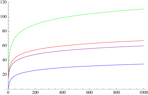
Figure 1: Comparison of $K(d,\infty)$ obtained via the three proof methods: Blue (bottom) $=$ Nemirovski; Magenta and Red (middle) $=$ type 2 inequalities; Green (top) $=$ truncation and Bernstein inequality

6 Proofs.

6.1 Proofs for Section 2

Proof of (6).

In case of $r=\infty$, the asserted inequalities read

$$\|x\|_{\infty}\ \leq\ \|x\|_{q}\ \leq\ d^{1/q}\|x\|_{\infty}\quad\text{for}\ 1\leq q<\infty$$

and are rather obvious. For $1\leq q<r<\infty$, (6) is an easy consequence of Hölder’s inequality. $\Box$

Proof of Lemma 2.4.

In case of $r=2$, $V(f+g)$ is equal to $V(f)+DV(f,g)+V(g)$. In case of $r\geq 2$ and $\|f\|_{r}=0$, both $DV(f,g)$ and $\int h(f)g\,d\mu$ are equal to zero, and the asserted inequalities reduce to the trivial statement that $V(g)\leq(r-1)V(g)$. Thus let us restrict our attention to the case $r>2$ and $\|f\|_{r}>0$.

Note first that the mapping

$$\mathbb{R}\ni t\ \mapsto\ h_{t}:=|f+tg|^{r}$$

is pointwise twice continuously differentiable with derivatives

$$\dot{h}_{t} = r|f+tg|^{r-1}\mathrm{sign}(f+tg)g\ =\ r|f+tg|^{r-2}(f+tg)g,$$

$$\ddot{h}_{t} = r(r-1)|f+tg|^{r-2}g^{2}.$$

By means of the inequality $|x+y|^{b}\leq 2^{b-1}\bigl{(}|x|^{b}+|y|^{b}\bigr{)}$ for real numbers $x$, $y$ and $b\geq 1$, a consequence of Jensen’s inequality, we can conclude that for any bound $t_{o}>0$,

$$\max_{|t|\leq t_{o}}|\dot{h}_{t}| \leq r2^{r-2}\bigl{(}|f|^{r-1}|g|+t_{o}^{r-1}|g|^{r}\bigr{)},$$

$$\max_{|t|\leq t_{o}}|\ddot{h}_{t}| \leq r(r-1)2^{r-3}\bigl{(}|f|^{r-2}|g|^{2}+t_{o}^{r-2}|g|^{r}\bigr{)}.$$

The latter two envelope functions belong to $L_{1}(\mu)$. This follows from Hölder’s inequality which we rephrase for our purposes in the form

$$\int|f|^{(1-\lambda)r}|g|^{\lambda r}\,d\mu\ \leq\ \|f\|_{r}^{(1-\lambda)r}\|g\|_{r}^{\lambda r}\quad\text{for}\ 0\leq\lambda\leq 1.$$ (17)

Hence we may conclude via dominated convergence that

$$t\ \mapsto\ \tilde{v}(t):=\|f+tg\|_{r}^{r}$$

is twice continuously differentiable with derivatives

$$\tilde{v}^{\prime}(t) = r\int|f+tg|^{r-2}(f+tg)g\,d\mu,$$

$$\tilde{v}^{\prime\prime}(t) = r(r-1)\int|f+tg|^{r-2}g^{2}\,d\mu.$$

This entails that

$$t\ \mapsto\ v(t):=V(f+tg)\ =\ \tilde{v}(t)^{2/r}$$

is continuously differentiable with derivative

$$v^{\prime}(t)\ =\ (2/r)\tilde{v}(t)^{2/r-1}\tilde{v}^{\prime}(t)\ =\ \tilde{v}^{2/r-1}(t)\int h(f+tg)g\,d\mu.$$

For $t=0$ this entails the asserted expression for $DV(f,g)$. Moreover, $v(t)$ is twice continuously differentiable on the set $\{t\in\mathbb{R}:\|f+tg\|_{r}>0\}$ which equals either $\mathbb{R}$ or $\mathbb{R}\setminus\{t_{o}\}$ for some $t_{o}\neq 0$. On this set the second derivative equals

$$v^{\prime\prime}(t) = (2/r)\tilde{v}(t)^{2/r-1}\tilde{v}^{\prime\prime}(t)+(2/r)(2/r-1)\tilde{v}(t)^{2/r-2}\tilde{v}^{\prime}(t)^{2}$$

$$= 2(r-1)\int\frac{|f+tg|^{r-2}}{\|f+tg\|_{r}^{r-2}}g^{2}\,d\mu-2(r-2)\Bigl{(}\int\frac{|f+tg|^{r-2}(f+tg)}{\|f+tg\|_{r}^{r-1}}g\,d\mu\Bigr{)}^{2}$$

$$\leq 2(r-1)\int\Bigl{|}\frac{f+tg}{\|f+tg\|_{r}}\Bigr{|}^{r-2}|g|^{2}\,d\mu$$

$$\leq 2(r-1)\|g\|_{r}^{2}\ =\ 2(r-1)V(g)$$

by virtue of Hölder’s inequality (17) with $\lambda=2/r$. Consequently, by using

$$v^{\prime}(t)-v^{\prime}(0)=\int_{0}^{t}v^{\prime\prime}(s)\,ds\leq 2(r-1)V(g)t,$$

we find that

$$V(f+g)-V(f)-DV(f,g)$$

$$= v(1)-v(0)-v^{\prime}(0)=\int_{0}^{1}(v^{\prime}(t)-v^{\prime}(0))\,dt$$

$$\leq 2(r-1)V(g)\int_{0}^{1}t\,dt=(r-1)V(g).$$

$\Box$

Proof of Theorem 2.2.

The first part is an immediate consequence of the considerations preceding the theorem. It remains to prove the (in)equalities and expansion for $K_{\rm Nem}(d,r)$. Note that $K_{\rm Nem}(d,r)$ is the infimum of $h(q)d^{-2/r}$ over all real $q\in[2,r]$, where $h(q):=(q-1)d^{2/q}$ satisfies the equation

$$h^{\prime}(q)\ =\ \frac{d^{2/q}}{q^{2}}\bigl{(}(q-\log d)^{2}-(\log d-2)\log d\bigr{)}.$$

Since $7<e^{2}<8$, this shows that $h$ is strictly increasing on $[2,\infty)$ if $d\leq 7$. Hence

$$K_{\rm Nem}(d,r)\ =\ h(2)d^{-2/r}\ =\ d^{1-2/r}\quad\text{if}\ d\leq 7.$$

For $d\geq 8$, one can easily show that $\log d-\sqrt{(\log d-2)\log d}<2$, so that $h$ is strictly decreasing on $[2,r_{d}]$ and strictly increasing on $[r_{d},\infty)$, where

$$r_{d}\ :=\ \log d+\sqrt{(\log d-2)\log d}\ \begin{cases}<\ 2\log d,\\ >\ 2\log d-2.\end{cases}$$

Thus for $d\geq 8$,

$$K_{\rm Nem}(d,r)\ =\ \begin{cases}h(r)d^{-2/r}\ =\ r-1\ <\ 2\log d-1&\text{if}\ r\leq r_{d},\\ h(r_{d})d^{-2/r}\ \leq\ h(2\log d)\ =\ 2e\log d-e&\text{if}\ r\geq r_{d}.\end{cases}$$

Moreover, one can verify numerically that $K_{\rm Nem}(d,r)\leq d\leq 2e\log d-e$ for $3\leq d\leq 7$.

Finally, for $d\geq 8$, the inequalities $r_{d}^{\prime}:=2\log d-2<r_{d}<r_{d}^{\prime\prime}:=2\log d$ yield

$$K_{\rm Nem}(d,\infty)=h(r_{d})\ \geq\ (r_{d}^{\prime}-1)d^{2/r_{d}^{\prime\prime}}\ =\ 2e\log d-3e,$$

and for $1\leq d\leq 7$, the inequality $d=K_{\rm Nem}(d,\infty)\geq 2e\log(d)-3e$ is easily verified. $\Box$

6.2 Proofs for Section 3

Proof of Lemma 3.2.

The following proof is standard; see e.g. [1], page 160, [13], page 247. Let $x_{1},\ldots,x_{n}$ be fixed functions in $L_{r}(\mu)$. Then by [8], for any $t\in T$,

$$\biggl{\{}\mathop{\rm I\!E}\nolimits\Bigl{|}\sum_{i=1}^{n}\epsilon_{i}x_{i}(t)\Bigr{|}^{r}\biggr{\}}^{1/r}\ \leq\ B_{r}\Bigl{(}\sum_{i=1}^{n}|x_{i}(t)|^{2}\Bigr{)}^{1/2}.$$ (18)

To use inequality (18) for finding an upper bound for the type constant for $L_{r}$, rewrite it as

$$\mathop{\rm I\!E}\nolimits\Bigl{|}\sum_{i=1}^{n}\epsilon_{i}x_{i}(t)\Bigr{|}^{r}\ \leq\ B_{r}^{r}\Bigl{(}\sum_{i=1}^{n}|x_{i}(t)|^{2}\Bigr{)}^{r/2}.$$

It follows from Fubini’s theorem and the previous inequality that

$$\mathop{\rm I\!E}\nolimits\Bigl{\|}\sum_{i=1}^{n}\epsilon_{i}x_{i}\Bigr{\|}_{r}^{r} = \mathop{\rm I\!E}\nolimits\int\Bigl{|}\sum_{i=1}^{n}\epsilon_{i}x_{i}(t)\Bigr{|}^{r}\,d\mu(t)$$

$$= \int\mathop{\rm I\!E}\nolimits\Bigl{|}\sum_{i=1}^{n}\epsilon_{i}x_{i}(t)|^{r}\,d\mu(t)$$

$$\leq B_{r}^{r}\int\biggl{(}\sum_{i=1}^{n}|x_{i}(t)|^{2}\biggr{)}^{r/2}\,d\mu(t).$$

Using the triangle inequality (or Minkowski’s inequality), we obtain

$$\biggl{\{}\mathop{\rm I\!E}\nolimits\Bigl{\|}\sum_{i=1}^{n}\epsilon_{i}x_{i}\Bigr{\|}_{r}^{r}\biggr{\}}^{2/r} \leq B_{r}^{2}\biggl{\{}\int\Bigl{(}\sum_{i=1}^{n}|x_{i}(t)|^{2}\Bigr{)}^{r/2}\,d\mu(t)\biggr{\}}^{2/r}$$

$$\leq B_{r}^{2}\sum_{i=1}^{n}\Bigl{(}\int|x_{i}(t)|^{r}\,d\mu(t)\Bigr{)}^{2/r}$$

$$= B_{r}^{2}\sum_{i=1}^{n}\|x_{i}\|_{r}^{2}.$$

Furthermore, since $g(v)=v^{2/r}$ is a concave function of $v\geq 0$, the last display implies that

$$\mathop{\rm I\!E}\nolimits\Bigl{\|}\sum_{i=1}^{n}\epsilon_{i}x_{i}\Bigr{\|}_{r}^{2}\ \leq\ \biggl{\{}\mathop{\rm I\!E}\nolimits\Bigl{\|}\sum_{i=1}^{n}\epsilon_{i}x_{i}\Bigr{\|}_{r}^{r}\biggr{\}}^{2/r}\ \leq\ B_{r}^{2}\sum_{i=1}^{n}\|x_{i}\|_{r}^{2}.$$

Proof of Lemma 3.4.

For $1\leq i\leq n$ let $x_{i}=(x_{im})_{m=1}^{d}$ be an arbitrary fixed vector in $\mathbb{R}^{d}$, and set $S:=\sum_{i=1}^{n}\epsilon_{i}x_{i}$. Further let $S_{m}$ be the $m$-th component of $S$ with variance $v_{m}^{2}:=\sum_{i=1}^{n}x_{im}^{2}$, and define $v^{2}:=\max_{1\leq m\leq d}v_{m}^{2}$, which is not greater than $\sum_{i=1}^{n}\|x_{i}\|_{\infty}^{2}$. It suffices to show that

$$\mathop{\rm I\!E}\nolimits\|S\|_{\infty}^{2}\ \leq\ 2\log(2d)v^{2}.$$

To this end note first that $h:[0,\infty)\to[1,\infty)$ with $h(t):=\cosh(t^{1/2})=\sum_{k=0}^{\infty}t^{k}/(2k)!$ is bijective, increasing and convex. Hence its inverse function $h^{-1}:[1,\infty)\to[0,\infty)$ is increasing and concave, and one easily verifies that $h^{-1}(s)=\bigl{(}\log(s+(s^{2}-1)^{1/2})\bigr{)}^{2}\leq(\log(2s))^{2}$. Thus it follows from Jensen’s inequality that for arbitrary $t>0$,

$$\mathop{\rm I\!E}\nolimits\|S\|_{\infty}^{2} = t^{-2}\mathop{\rm I\!E}\nolimits h^{-1}\bigl{(}\cosh(\|tS\|_{\infty})\bigr{)}\ \leq\ t^{-2}h^{-1}\bigl{(}\mathop{\rm I\!E}\nolimits\cosh(\|tS\|_{\infty})\bigr{)}$$

$$\leq t^{-2}\bigl{(}\log\bigl{(}2\mathop{\rm I\!E}\nolimits\cosh(\|tS\|_{\infty})\bigr{)}\bigr{)}^{2}.$$

Moreover,

$$\mathop{\rm I\!E}\nolimits\cosh(\|tS\|_{\infty})\ =\ \mathop{\rm I\!E}\nolimits\max_{1\leq m\leq d}\cosh(tS_{m})\ \leq\ \sum_{m=1}^{d}\mathop{\rm I\!E}\nolimits\cosh(tS_{m})\ \leq\ d\exp(t^{2}v^{2}/2),$$

according to (8), whence

$$\mathop{\rm I\!E}\nolimits\|S\|_{\infty}^{2}\ \leq\ t^{-2}\log\bigl{(}2d\exp(t^{2}v^{2}/2)\bigr{)}^{2}\ =\ \bigl{(}\log(2d)/t+tv^{2}/2\bigr{)}^{2}.$$

Now the assertion follows if we set $t=\sqrt{2\log(2d)/v^{2}}$. $\Box$

Proof of (9).

We may replace the random sequence $\{X_{i}\}$ in Example 1.2 with the random sequence $\{\epsilon_{i}X_{i}\}$, where $\{\epsilon_{i}\}$ is a Rademacher sequence independent of $\{X_{i}\}$. Thereafter we condition on $\{X_{i}\}$, i.e. we view it as a deterministic sequence such that $n^{-1}\sum_{i=1}^{n}X_{i}X_{i}^{\top}$ converges to the identity matrix $I_{d}$ as $n\to\infty$, by the strong law of large numbers. Now Lindeberg’s version of the multivariate Central Limit Theorem shows that

$$\sup_{n\geq 1}\frac{\mathop{\rm I\!E}\nolimits\Bigl{\|}\sum_{i=1}^{n}\epsilon_{i}X_{i}\Bigr{\|}_{\infty}^{2}}{\sum_{i=1}^{n}\|X_{i}\|_{\infty}^{2}}\ \geq\ \sup_{n\geq 1}\mathop{\rm I\!E}\nolimits\Bigl{\|}n^{-1/2}\sum_{i=1}^{n}\epsilon_{i}X_{i}\Bigr{\|}_{\infty}^{2}\ \geq\ c_{d}^{2}.$$

Inequalities for $\Phi$.

The subsequent results will rely on (10) and several inequalities for $1-\Phi(z)$. The first of these is:

$$1-\Phi(z)\leq z^{-1}\phi(z),\qquad z>0,$$ (19)

which is known as Mills’ ratio; see [6] and [19] for related results. The proof of this upper bound is easy: Since $\phi^{\prime}(z)=-z\phi(z)$ it follows that

$$1-\Phi(z)=\int_{z}^{\infty}\phi(t)\,dt\leq\int_{z}^{\infty}\frac{t}{z}\phi(t)\,dt=\frac{-1}{z}\int_{z}^{\infty}\phi^{\prime}(t)\,dt=\frac{\phi(z)}{z}.$$ (20)

A very useful pair of upper and lower bounds for $1-\Phi(z)$ are as follows:

$$\frac{2}{z+\sqrt{z^{2}+4}}\phi(z)\leq 1-\Phi(z)\leq\frac{4}{3z+\sqrt{z^{2}+8}}\phi(z),\qquad z>-1;$$ (21)

the inequality on the left is due to Komatsu (see e.g. [10] p. 17), while the inequality on the right is an improvement of an earlier result of Komatsu due to [23].

Proof of Lemma 3.6.

To prove the upper bound for $T_{2}(\ell_{\infty}^{d})$, let $(\epsilon_{i})_{i\geq 1}$ be a Rademacher sequence. With $S$ and $S_{m}$ as in the proof of Lemma 3.4, we may write

$$\mathop{\rm I\!E}\nolimits\|S\|_{\infty}^{2} = \int_{0}^{\infty}2t\mathop{\rm I\!P}\nolimits\Big{(}\sup_{1\leq m\leq d}|S_{m}|>t\Big{)}\,dt$$

$$\leq \delta^{2}+\int_{\delta}^{\infty}2t\mathop{\rm I\!P}\nolimits\Big{(}\sup_{1\leq m\leq d}|S_{m}|>t\Big{)}\,dt$$

$$\leq \delta^{2}+\sum_{m=1}^{d}\int_{\delta}^{\infty}2t\mathop{\rm I\!P}\nolimits\big{(}|S_{m}|>t\big{)}\,dt.$$

Now by (10) with $v^{2}$ and $v_{m}^{2}$ as in the proof of Lemma 3.4, followed by Mills’ ratio (19),

$$\int_{\delta}^{\infty}2t\mathop{\rm I\!P}\nolimits(|S_{m}|>t)\,dt \leq \int_{\delta}^{\infty}\frac{4Kv_{m}}{\sqrt{2\pi}t}te^{-t^{2}/(2v_{m}^{2})}\,dt$$ (22)

$$= \frac{4Kv_{m}}{\sqrt{2\pi}}\int_{\delta}^{\infty}e^{-t^{2}/(2v_{m}^{2})}\,dt\ =\ 4Kv_{m}^{2}\int_{\delta}^{\infty}\frac{e^{-t^{2}/(2v_{m}^{2})}}{\sqrt{2\pi}v_{m}}\,dt$$

$$= 4Kv_{m}^{2}(1-\Phi(\delta/v_{m}))\ \leq\ 4Kv^{2}(1-\Phi(\delta/v)).$$

Now instead of the Mills’ ratio bound (19) for the tail of the normal distribution, we use the upper bound part of (21) due to [23]. This yields

$$\int_{\delta}^{\infty}2t\mathop{\rm I\!P}\nolimits(|S_{m}|>t)\,dt\leq 4Kv^{2}(1-\Phi(\delta/v))\leq\frac{4cv^{2}}{3\delta/v+\sqrt{\delta^{2}/v^{2}+8}}e^{-\delta^{2}/(2v^{2})},$$

where we have defined $c:=4K/\sqrt{2\pi}=12.88/\sqrt{2\pi}$, and hence

$$\mathop{\rm I\!E}\nolimits\|S\|^{2}\leq\delta^{2}+\frac{4cdv^{2}}{3\delta/v+\sqrt{\delta^{2}/v^{2}+8}}e^{-\delta^{2}/(2v^{2})}.$$

Taking

$$\delta^{2}=v^{2}2\log\left(\frac{cd/2}{\sqrt{2\log(cd/2)}}\right)$$

gives

$$\mathop{\rm I\!E}\nolimits\|S\|^{2} \leq v^{2}\Biggl{\{}2\log d+2\log(c/2)-\log(2\log(dc/2))$$

$$\qquad\qquad+\ \ \frac{8\sqrt{2\log(cd/2)}}{3\sqrt{2\log\big{(}\frac{cd}{2\sqrt{2\log(cd/2)}}\big{)}}+\sqrt{2\log\big{(}\frac{cd}{2\sqrt{2\log(cd/2)}}\big{)}+8}}\Biggr{\}}$$

$$=: v^{2}\{2\log d+h_{2}(d)\}$$

where it is easily checked that $h_{2}(d)\leq 3$ for all $d\geq 1$. Moreover $h_{2}(d)$ is negative for $d>4.13795*10^{10}$. This completes the proof of the upper bound in (14).

To prove the lower bound for $c_{d}$ in (14), we use the lower bound of [13], Lemma 6.9, page 157 (which is, in this form, due to [5]). This yields

$$c_{d}^{2}\geq\frac{\lambda}{1+\lambda}t_{o}^{2}+\frac{1}{1+\lambda}d\int_{t_{o}}^{\infty}4t(1-\Phi(t))\,dt$$ (23)

for any $t_{o}>0$, where $\lambda=2d(1-\Phi(t_{o}))$. By using Komatsu’s lower bound (21), we find that

$$\int_{t_{o}}^{\infty}t(1-\Phi(t))\,dt \geq \int_{t_{o}}^{\infty}\frac{2t}{t+\sqrt{t^{2}+4}}\phi(t)\,dt$$

$$\geq \frac{2t_{o}}{t_{o}+\sqrt{t_{o}^{2}+4}}\int_{t_{o}}^{\infty}\phi(t)\,dt$$

$$= \frac{2}{1+\sqrt{1+4/t_{o}^{2}}}(1-\Phi(t_{o})).$$

Using this lower bound in (23) yields

$$c_{d}^{2} \geq \frac{\lambda}{1+\lambda}t_{o}^{2}+\frac{1}{1+\lambda}d\frac{8}{1+\sqrt{1+4/t_{o}^{2}}}(1-\Phi(t_{o}))$$ (24)

$$= \frac{2d(1-\Phi(t_{o}))}{1+2d(1-\Phi(t_{o}))}\left\{t_{o}^{2}+\frac{4}{1+\sqrt{1+4/t_{o}^{2}}}\right\}$$

$$\geq \frac{\frac{4d}{t_{o}+\sqrt{t_{o}^{2}+4}}\phi(t_{o})}{1+\frac{4d}{t_{o}+\sqrt{t_{o}^{2}+4}}\phi(t_{o})}\left\{t_{o}^{2}+\frac{4}{1+\sqrt{1+4/t_{o}^{2}}}\right\}.$$

Now we let $c\equiv\sqrt{2/\pi}$ and $\delta>0$ and choose

$$t_{o}^{2}=2\log\left(\frac{cd}{(2\log(cd))^{(1+\delta)/2}}\right).$$

For this choice we see that $t_{o}\rightarrow\infty$ as $d\rightarrow\infty$,

$$4d\phi(t_{o})=\frac{2d}{\sqrt{2\pi}}\cdot\frac{(2\log(cd))^{(1+\delta)/2}}{cd}=2(2\log(cd))^{(1+\delta)/2},$$

and

$$\frac{4d\phi(t_{o})}{t_{o}}=\frac{2(2\log(cd))^{(1+\delta)/2}}{\{2\log(cd/(2\log(cd))^{(1+\delta)/2})\}^{1/2}}\to\infty$$

as $d\to\infty$, so the first term on the RHS of (24) converges to $1$ as $d\rightarrow\infty$, and it can be rewritten as

$$A_{d}\left\{t_{o}^{2}+\frac{4}{1+\sqrt{1+4/t_{o}^{2}}}\right\}$$

$$= A_{d}\left\{2\log\left(\frac{cd}{(2\log(cd))^{(1+\delta)/2}}\right)+\frac{4}{1+\sqrt{1+4/t_{o}^{2}}}\right\}$$

$$\sim 1\cdot\left\{2\log d+2\log c-(1+\delta)\log(2\log(cd))+2\right\}.$$

To prove the upper bounds for $c_{d}$, we will use the upper bound of [13], Lemma 6.9, page 157 (which is, in this form, due to [5]). For every $t_{o}>0$

$$c_{d}^{2}\equiv\mathop{\rm I\!E}\nolimits\max_{1\leq j\leq d}|Z_{j}|^{2} \leq t_{o}^{2}+d\int_{t_{o}}^{\infty}2tP(|Z_{1}|>t)dt$$

$$= t_{o}^{2}+4d\int_{t_{o}}^{\infty}t(1-\Phi(t))dt$$

$$\leq t_{o}^{2}+4d\int_{t_{o}}^{\infty}\phi(t)dt\qquad(\text{by Mills' ratio})$$

$$= t_{o}^{2}+4d(1-\Phi(t_{o})).$$

Evaluating this bound at $t_{o}=\sqrt{2\log(d/\sqrt{2\pi})}$ and then using Mills’ ratio again yields

$$c_{d}^{2} \leq 2\log(d/\sqrt{2\pi})+4d(1-\Phi(\sqrt{2\log(d/\sqrt{2\pi})}))$$

$$\leq 2\log d-2\frac{1}{2}\log(2\pi)+4d\frac{\phi(\sqrt{2\log(d/\sqrt{2\pi})})}{\sqrt{2\log(d/\sqrt{2\pi})}}$$

$$= 2\log d-\log(2\pi)+\frac{2\sqrt{2}}{\sqrt{\log(d/\sqrt{2\pi})}}$$

$$\leq 2\log d$$

where the last inequality holds if

$$\frac{2\sqrt{2}}{\sqrt{\log(d/\sqrt{2\pi})}}\leq\log(2\pi),$$

or equivalently if

$$\log d\ \geq\ \frac{8}{(\log(2\pi))^{2}}+\frac{\log(2\pi)}{2}\ =\ 3.28735...,$$

and hence if $d\geq 27>e^{3.28735...}\ \dot{=}\ 26.77$. The claimed inequality is easily verified numerically for $d=3,\ldots,26$. (It fails for $d=2$.) As can be seen from (6.2), $2\log d-\log(2\pi)$ gives a reasonable approximation to $\mathop{\rm I\!E}\nolimits\max_{1\leq j\leq d}Z_{j}^{2}$ for large $d$. Using the upper bound in (21) instead of the second application of Mills’ ratio and choosing $t_{o}^{2}=2\log(cd/\sqrt{2\log(cd)})$ with $c\ :=\ \sqrt{2/\pi}$ yields the third bound for $c_{d}$ in (14) with

$$h_{3}(d) = -\log(\pi)-\log(\log(cd))$$

$$\ \ +\ \frac{8}{3\sqrt{1-\frac{\log(2\log(cd))}{2\log(cd)}}+\sqrt{1-\frac{\log(2\log(cd))}{2\log(cd)}+\frac{4}{\log(cd)}}}.$$

$\Box$

6.3 Proofs for Section 4

Proof of Lemma 4.1.

It follows from $\mathop{\rm I\!E}\nolimits Z=0$, the Taylor expansion of the exponential function and the inequality $\mathop{\rm I\!E}\nolimits|Z|^{m}\leq\sigma^{2}\kappa^{m-2}$ for $m\geq 2$ that

$$\mathop{\rm I\!E}\nolimits\exp\Bigl{(}\frac{Z}{\kappa L}\Bigr{)}\ =\ 1+\mathop{\rm I\!E}\nolimits\Bigl{\{}\exp\Bigl{(}\frac{Z}{\kappa L}\Bigr{)}-1-\frac{Z}{\kappa L}\Bigr{\}}$$

$$\leq 1+\sum_{m=2}^{\infty}\frac{1}{m!}\frac{\mathop{\rm I\!E}\nolimits|Z|^{m}}{(\kappa L)^{m}}\ \leq\ 1+\frac{\sigma^{2}}{\kappa^{2}}\sum_{m=2}^{\infty}\frac{1}{m!}\frac{1}{L^{m}}\ =\ 1+\frac{\sigma^{2}{\rm e}(L)}{\kappa^{2}}.$$

$\Box$

Proof of Lemma 4.2.

Applying Lemma 4.1 to the $j$-th components $X_{i,j}$ of $X_{i}$ and $S_{n,j}$ of $S_{n}$ yields for all $L>0$,

$$\mathop{\rm I\!E}\nolimits\exp\Bigl{(}\frac{\pm S_{n,j}}{\kappa L}\Bigr{)}\ =\ \prod_{i=1}^{n}\mathop{\rm I\!E}\nolimits\exp\Bigl{(}\frac{\pm X_{i,j}}{\kappa L}\Bigr{)}\ \leq\ \prod_{i=1}^{n}\exp\Bigl{(}\frac{\mathop{\rm Var}\nolimits(X_{i,j}){\rm e}(L)}{\kappa^{2}}\Bigr{)}\ \leq\ \exp\Bigl{(}\frac{\Gamma{\rm e}(L)}{\kappa^{2}}\Bigr{)}.$$

Hence

$$\mathop{\rm I\!E}\nolimits\cosh\Bigl{(}\frac{\|S_{n}\|_{\infty}}{\kappa L}\Bigr{)}\ =\ \mathop{\rm I\!E}\nolimits\max_{1\leq j\leq d}\cosh\Bigl{(}\frac{S_{n,j}}{\kappa L}\Bigr{)}\ \leq\ \sum_{j=1}^{d}\mathop{\rm I\!E}\nolimits\cosh\Bigl{(}\frac{S_{n,j}}{\kappa L}\Bigr{)}\ \leq\ d\exp\Bigl{(}\frac{\Gamma{\rm e}(L)}{\kappa^{2}}\Bigr{)}.$$

As in the proof of Lemma 3.4 we conclude that

$$\mathop{\rm I\!E}\nolimits\|S_{n}\|_{\infty}^{2} \leq (\kappa L)^{2}\biggl{(}\log\Bigl{(}2\mathop{\rm I\!E}\nolimits\cosh\Bigl{(}\frac{\|S_{n}\|_{\infty}}{\kappa L}\Bigr{)}\Bigr{)}\biggr{)}^{2}$$

$$\leq (\kappa L)^{2}\Bigl{(}\log(2d)+\frac{\Gamma{\rm e}(L)}{\kappa^{2}}\Bigr{)}^{2}$$

$$= \Bigl{(}\kappa L\log(2d)+\frac{\Gamma L\,{\rm e}(L)}{\kappa}\Bigr{)}^{2},$$

which is equivalent to the inequality stated in the lemma. $\Box$

Proof of Theorem 4.3.

For fixed $\kappa_{o}>0$ we split $S_{n}$ into $A_{n}+B_{n}$ as described before. Let us bound the sum $B_{n}$ first: For this term we have

$$\|B_{n}\|_{\infty} \leq \sum_{i=1}^{n}\bigl{\{}1_{[\|X_{i}\|_{\infty}>\kappa_{o}]}\|X_{i}\|_{\infty}+\mathop{\rm I\!E}\nolimits(1_{[\|X_{i}\|_{\infty}>\kappa_{o}]}\|X_{i}\|_{\infty})\bigr{\}}$$

$$= \sum_{i=1}^{n}\bigl{\{}1_{[\|X_{i}\|_{\infty}>\kappa_{o}]}\|X_{i}\|_{\infty}-\mathop{\rm I\!E}\nolimits(1_{[\|X_{i}\|_{\infty}>\kappa_{o}]}\|X_{i}\|_{\infty})\bigr{\}}$$

$$\qquad+\ 2\sum_{i=1}^{n}\mathop{\rm I\!E}\nolimits(1_{[\|X_{i}\|_{\infty}>\kappa_{o}]}\|X_{i}\|_{\infty})$$

$$=: B_{n1}+B_{n2}.$$

Therefore, since $\mathop{\rm I\!E}\nolimits B_{n1}=0$,

$$\mathop{\rm I\!E}\nolimits\|B_{n}\|_{\infty}^{2} \leq \mathop{\rm I\!E}\nolimits(B_{n1}+B_{n2})^{2}\ =\ \mathop{\rm I\!E}\nolimits B_{n1}^{2}+B_{n2}^{2}$$

$$= \sum_{i=1}^{n}\mathop{\rm Var}\nolimits\bigl{(}1_{[\|X_{i}\|_{\infty}>\kappa_{o}]}\|X_{i}\|_{\infty}\bigr{)}+4\Bigl{(}\sum_{i=1}^{n}\mathop{\rm I\!E}\nolimits(\|X_{i}\|_{\infty}1_{[\|X_{i}\|_{\infty}>\kappa_{o}]})\Bigr{)}^{2}$$

$$\leq \sum_{i=1}^{n}\mathop{\rm I\!E}\nolimits\|X_{i}\|_{\infty}^{2}+4\Bigl{(}\sum_{i=1}^{n}\frac{\mathop{\rm I\!E}\nolimits\|X_{i}\|_{\infty}^{2}}{\kappa_{o}}\Bigr{)}^{2}$$

$$= \Gamma+4\frac{\Gamma^{2}}{\kappa_{o}^{2}},$$

where we define $\Gamma:=\sum_{i=1}^{n}\mathop{\rm I\!E}\nolimits\|X_{i}\|_{\infty}^{2}$.

The first sum, $A_{n}$, may be bounded by means of Lemma 4.2 with $\kappa=2\kappa_{o}$, utilizing the bound

$$\mathop{\rm Var}\nolimits(X_{i,j}^{(a)})\ =\ \mathop{\rm Var}\nolimits\bigl{(}1_{[\|X_{i}\|_{\infty}\leq\kappa_{o}]}X_{i,j}\bigr{)}\ \leq\ \mathop{\rm I\!E}\nolimits\bigl{(}1_{[\|X_{i}\|_{\infty}\leq\kappa_{o}]}X_{i,j}^{2}\bigr{)}\ \leq\ \mathop{\rm I\!E}\nolimits\|X_{i}\|_{\infty}^{2}.$$

Thus

$$\mathop{\rm I\!E}\nolimits\|A_{n}\|_{\infty}^{2}\ \leq\ \Bigl{(}2\kappa_{o}L\log(2d)+\frac{\Gamma L\,{\rm e}(L)}{2\kappa_{o}}\Bigr{)}^{2}.$$

Combining the bounds we find that

$$\sqrt{\mathop{\rm I\!E}\nolimits\|S_{n}\|_{\infty}^{2}} \leq \sqrt{\mathop{\rm I\!E}\nolimits\|A_{n}\|_{\infty}^{2}}+\sqrt{\mathop{\rm I\!E}\nolimits\|B_{n}\|_{\infty}^{2}}$$

$$\leq 2\kappa_{o}L\log(2d)+\frac{\Gamma L{\rm e}(L)}{2\kappa_{o}}+\ \sqrt{\Gamma}+2\frac{\Gamma}{\kappa_{o}}$$

$$= \alpha\kappa_{o}+\frac{\beta}{\kappa_{o}}+\sqrt{\Gamma},$$

where $\alpha:=2L\log(2d)$ and $\beta:=\Gamma(L\,{\rm e}(L)+4)/2$. This bound is minimized if $\kappa_{o}=\sqrt{\beta/\alpha}$ with minimum value

$$2\sqrt{\alpha\beta}+\sqrt{\Gamma}\ =\ \bigl{(}1+2\sqrt{L^{2}{\rm e}(L)+4L}\sqrt{\log(2d)}\bigr{)}\sqrt{\Gamma},$$

and for $L=0.407$ the latter bound is not greater than

$$\bigl{(}1+3.46\sqrt{\log(2d)}\bigr{)}\sqrt{\Gamma}.$$

In the special case of symmetrically distributed random vectors $X_{i}$, our treatment of the sum $B_{n}$ does not change, but in the bound for $\mathop{\rm I\!E}\nolimits\|A_{n}\|_{\infty}^{2}$ one may replace $2\kappa_{o}$ with $\kappa_{o}$, because $\mathop{\rm I\!E}\nolimits X_{i}^{(a)}=0$. Thus

$$\sqrt{\mathop{\rm I\!E}\nolimits\|S_{n}\|_{\infty}^{2}} \leq \kappa_{o}L\log(2d)+\frac{\Gamma L{\rm e}(L)}{\kappa_{o}}+\ \sqrt{\Gamma}+2\frac{\Gamma}{\kappa_{o}}$$

$$= \alpha^{\prime}\kappa_{o}+\frac{\beta^{\prime}}{\kappa_{o}}+\sqrt{\Gamma}\qquad\bigl{(}\text{with}\ \alpha^{\prime}:=L\log(2d),\beta^{\prime}:=\Gamma(L\,{\rm e}(L)+2)\bigr{)}$$

$$= \bigl{(}1+2\sqrt{L^{2}{\rm e}(L)+2L}\sqrt{\log(2d)}\bigr{)}\sqrt{\Gamma}\qquad\bigl{(}\text{if}\ \kappa_{o}=\sqrt{\beta^{\prime}/\alpha^{\prime}}\bigr{)}.$$

For $L=0.5$ the latter bound is not greater than

$$\bigl{(}1+2.9\sqrt{\log(2d)}\bigr{)}\sqrt{\Gamma}.$$

Acknowledgements.

The authors owe thanks to the referees for a number of suggestions which resulted in a considerable improvement in the article. The authors are also grateful to Ilya Molchanov for drawing their attention to Banach-Mazur distances, and to Stanislaw Kwapien and Vladimir Koltchinskii for pointers concerning type and co-type proofs and constants. This research was initiated during the opening week of the program on “Statistical Theory and Methods for Complex, High-Dimensional Data” held at the Isaac Newton Institute for Mathematical Sciences from 7 January to 27 June, 2008, and was made possible in part by the support of the Isaac Newton Institute for visits of various periods by Dümbgen, van de Geer, and Wellner. The research of Wellner was also supported in part by NSF grants DMS-0503822 and DMS-0804587. The research of Dümbgen and van de Geer was supported in part by the Swiss National Science Foundation.

Lutz Dümbgen received his Ph.D. from Heidelberg University in 1990. From 1990-1992 he was a Miller research fellow at the University of California at Berkeley. Thereafter he worked at the universities of Bielefeld, Heidelberg and Lübeck. Since 2002 he is professor of statistics at the University of Bern. His research interests are nonparametric, multivariate and computational statistics.

Institute of Mathematical Statistics and Actuarial Science, University of Bern, Alpeneggstrasse 22, CH-3012 Bern, Switzerland
duembgen@stat.unibe.ch

Sara A. van de Geer obtained her Ph.D. at Leiden University in 1987. She worked at the Center for Mathematics and Computer Science in Amsterdam, at the Universities of Bristol, Utrecht, Leiden and Toulouse, and at the Eidgenössische Technische Hochschule in Zürich (2005-present). Her research areas are empirical processes, statistical learning, and statistical theory for high-dimensional data.

Seminar for Statistics, ETH Zurich, CH-8092 Zurich, Switzerland
geer@stat.math.ethz.ch

Mark C. Veraar received his Ph.D. from Delft University of Technology in 2006. In the year 2007 he stayed as a PostDoc researcher in the European RTN project “Phenomena in High Dimensions” at the IMPAN institute in Warsaw (Poland). In 2008 he spent one year as an Alexander von Humboldt fellow at the University of Karlsruhe (Germany). Since 2009 he is Assistant Professor at Delft University of Technology (the Netherlands). His main research areas are probability theory, partial differential equations and functional analysis.

Delft Institute of Applied Mathematics, Delft University of Technology, P.O. Box 5031, 2600 GA Delft, The Netherlands
m.c.veraar@tudelft.nl, mark@profsonline.nl

Jon A. Wellner received his B.S. from the University of Idaho in 1968 and his Ph.D. from the University of Washington in 1975. He got hooked on research in probability and statistics during graduate school at the UW in the early 1970’s, and has enjoyed both teaching and research at the University of Rochester (1975-1983) and the University of Washington (1983-present). If not for probability theory and statistics, he might be a ski bum.

Department of Statistics, Box 354322, University of Washington, Seattle, WA 98195-4322
jaw@stat.washington.edu

References

- [1] A. Araujo and E. Giné, The central limit theorem for real and Banach valued random variables, John Wiley & Sons, New York-Chichester-Brisbane, 1980, Wiley Series in Probability and Mathematical Statistics.
- [2] G. Bennett, Probability inequalities for the sum of independent random variables, Journal of the American Statistical Association 57 (1962) 33–45.
- [3] V. H. de la Peña and E. Giné, Decoupling, Probability and its Applications (New York), Springer-Verlag, New York, 1999, From dependence to independence, Randomly stopped processes, -statistics and processes, Martingales and beyond.
- [4] R. M. Dudley, Uniform Central Limit Theorems, Cambridge Studies in Advanced Mathematics, vol. 63, Cambridge University Press, Cambridge, 1999.
- [5] E. Giné and J. Zinn, Central limit theorems and weak laws of large numbers in certain Banach spaces, Z. Wahrsch. Verw. Gebiete 62 (1983) 323–354.
- [6] R. D. Gordon, Values of Mills’ ratio of area to bounding ordinate and of the normal probability integral for large values of the argument, Ann. Math. Statistics 12 (1941) 364–366.
- [7] E. Greenshtein and Y. Ritov, Persistence in high-dimensional linear predictor selection and the virtue of overparametrization, Bernoulli 10 (2004) 971–988.
- [8] U. Haagerup, The best constants in the Khintchine inequality, Studia Math. 70 (1981) 231–283.
- [9] W. Hoeffding, Probability inequalities for sums of bounded random variables, J. Amer. Statist. Assoc. 58 (1963) 13–30.
- [10] K. Itô and H. P. McKean, Jr., Diffusion processes and their sample paths, Springer-Verlag, Berlin, 1974, Second printing, corrected, Die Grundlehren der mathematischen Wissenschaften, Band 125.
- [11] W. B. Johnson and J. Lindenstrauss, Basic concepts in the geometry of Banach spaces, in Handbook of the geometry of Banach spaces, Vol. I, North-Holland, Amsterdam, 2001, 1–84.
- [12] A. Juditsky and A. S. Nemirovski, Large deviations of vector-valued martingales in 2-smooth normed spaces, Tech. report, Georgia Institute of Technology, 2008.
- [13] M. Ledoux and M. Talagrand, Probability in Banach Spaces, Ergebnisse der Mathematik und ihrer Grenzgebiete (3) [Results in Mathematics and Related Areas (3)], vol. 23, Springer-Verlag, Berlin, 1991, Isoperimetry and processes.
- [14] A. S. Nemirovski, Topics in non-parametric statistics, in Lectures on Probability Theory and Statistics (Saint-Flour, 1998), Lecture Notes in Mathematics, vol. 1738, Springer, Berlin, 2000, 85–277.
- [15] , Regular Banach spaces and large deviations of random sums, Working paper, 2004.
- [16] A. S. Nemirovski and D. B. Yudin, Problem Complexity and Method Efficiency in Optimization, John Wiley and Sons, Chichester, 1983.
- [17] I. Pinelis, Extremal probabilistic problems and Hotelling’s test under a symmetry condition, Ann. Statist. 22 (1994) 357–368.
- [18] , Optimum bounds for the distributions of martingales in Banach spaces, Ann. Probab. 22 (1994) 1679–1706.
- [19] , Monotonicity properties of the relative error of a Padé approximation for Mills’ ratio, JIPAM. J. Inequal. Pure Appl. Math. 3 (2002) Article 20, 8 pp. (electronic).
- [20] , Toward the best constant factor for the Rademacher-Gaussian tail comparison, ESAIM Probab. Stat. 11 (2007) 412–426 (electronic).
- [21] D. Pollard, Empirical processes: theory and applications, NSF-CBMS Regional Conference Series in Probability and Statistics, 2, Institute of Mathematical Statistics, Hayward, CA, 1990.
- [22] E. Rio, Moment inequalities for sums of dependent random variables under projective conditions, J. Theor. Probab. 21 (2008) to appear.
- [23] S. J. Szarek and E. Werner, A nonsymmetric correlation inequality for Gaussian measure, J. Multivariate Anal. 68 (1999) 193–211.
- [24] N. Tomczak-Jaegermann, Banach-Mazur distances and finite-dimensional operator ideals, Pitman Monographs and Surveys in Pure and Applied Mathematics, vol. 38, Longman Scientific & Technical, Harlow, 1989.
- [25] S. A. van de Geer, Applications of empirical process theory, Cambridge Series in Statistical and Probabilistic Mathematics, vol. 6, Cambridge University Press, Cambridge, 2000.
- [26] A. W. van der Vaart and J. A. Wellner, Weak convergence and empirical processes, Springer Series in Statistics, Springer-Verlag, New York, 1996, With applications to statistics.