Ramsey interferometry with a spin embedded in a Coulomb chain

Abstract

We show that the statistical properties of a Coulomb crystal can be measured by means of a standard interferometric procedure performed on the spin of one ion in the chain. The ion spin, constituted by two internal levels of the ion, couples to the crystal modes via spatial displacement induced by photon absorption. The loss of contrast in the interferometric signal allows one to measure the autocorrelation function of the crystal observables. Close to the critical point, where the chain undergoes a second-order phase transition to a zigzag structure, the signal gives the behaviour of the correlation function at the critical point.

I Introduction

The quest for control of quantum dynamics of systems with increasing size is one of the present challenges in technological applications of quantum mechanics PZroadmap . It involves understanding the transition from the quantum to the classical world zurek-today and is based on the full knowledge of how the quantum properties scale with the system size, and in particular, of how the thermodynamic properties are related to the system microscopic dynamics FordKacMazur ; leggett-rmp ; weiss . Several experiments pursue a bottom-up approach, where systems of increasing complexity are built by combining together simpler systems, over which one has full control PZroadmap . In this context, Coulomb crystals of ions in Paul and Penning traps constitute a prominent system. These crystals are composed by cold ions in a confining potential that balances the Coulomb repulsion. The ions vibrate around fixed positions in analogy to the situation in an ordinary solid, while the interparticle distance is usually of the order of several micrometers, constituting an extremely rarefied type of condensed matter DubinRMP . Varying the potential permits one to control the number of ions, allowing one to explore structures of very different sizes, thus offering the opportunity of studying the dynamics from few particles to mesoscopic systems. Besides, these structures provide promising applications, among others, for quantum information processors QIPC:Ions ; QIPC:Ions:Exp and simulators Wunderlich ; Porras ; porras-spin-boson ; Schatz .

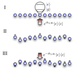
Figure 1: Color online. Ramsey interferometry with a chain. I. A transverse laser pulse prepares one ion of the chain in a superposition of the internal states $|g\rangle$ and $|e\rangle$. The mechanical effect, associated with the absorption of a laser photon and conditioned to the ion being in state $|e\rangle$, displaces the ion transversally and excites the modes of the chain. II. The chain is let freely evolve for a time $t$. III. A second laser pulse, addressing the same ion of the chain, is sent in the opposite direction of the first pulse. The probability that the ion is in state $|g\rangle$ is then measured as a function of $t$.

Among various crystalline structures experimentally realized Drewsen ; Bollinger ; Werth , low-dimensional structures, and in particular linear chains of ions, are routinely produced in ion trap laboratories. Linear chains are obtained in anisotropic potentials with large transverse confinement, usually linear Paul traps Ghosh , and can be composed by several dozens of ions. They exhibit a mechanical instability to a zigzag structure as a function of the ion number or of the transverse confinement, which has been first characterized experimentally in MPQ ; Raizen . The dynamics and thermodynamics of the linear chain have been extensively studied in several theoretical works DubinPRE ; Piacente ; morigi2004 . Most recently, it has been demonstrated that in the classical regime the mechanical instability of the linear chain, which leads to the abrupt transition to a zigzag structure, is a second order phase transition Dubin93 ; fishman2008 . The effects of quantum fluctuations on low-dimensional Wigner crystals have been discussed in Schulz , and are expected to be in general negligible for Coulomb crystals of atomic ions Yin . Most recently, in retzker parameter regimes have been discussed, where quantum effects in structures of few ions could be experimentally observed. These theoretical predictions lead to a practical issue, namely how to determine experimentally the thermodynamic quantities of large crystals. In fact, while the quantum state of few trapped ions is experimentally fully accessible by quantum tomographic techniques Leibfried96 ; Measure:Ion , the application of such technologies to larger crystals requires diverging experimental times.

In this paper, we discuss a method for measuring the dynamical and statistical properties of an ion chain, which is sketched in Fig. 1. This method is based on an extension of Ramsey interferometry with ions Ramsey ; Poyatos95 , which is applied to a dipolar transition of one ion belonging to the chain. This transition couples to the crystal modes via spatial displacement induced by photon absorption or emission. By measuring the interferometric contrast in a suitable setup, we show that one can directly measure the autocorrelation function of the crystal. In particular, we determine the dependence of the interferometric signal on the system size and on the distance of the control parameters from the critical point of the phase transition to the zigzag configuration. Based on the latter dependence, the interferometric signal may allow one to measure the critical exponents.

This work is organized as follows. The salient properties of Ramsey interferometry with ions in traps are reviewed in Sec. II. In Sec. III we introduce the system, composed by a Coulomb chain and the spin of one of the ions of the crystal. The interferometric signals obtained for this system are presented in Sec. IV. The conclusions are discussed in Sec. V. In the Appendix we report the details of calculations at the basis of the results presented in Sec. IV.

II Ramsey Interferometry with ions

Ramsey interferometry is routinely applied in quantum optics, nuclear magnetic resonance, atomic and molecular physics for high precision measurements Ramsey . Most recently, it has been considered for measuring the loss of coherence in quantum optical systems due to coupling with an external environment. Prominent experimental applications are in cavity quantum electrodynamics Ramsey:CQED and trapped ions Sackett . The idea at the basis of this implementation can be summarized as follows. Loss of coherence in quantum dynamics is often associated to the partition of a large quantum system into subsystems, of which only one part $S$ is fully controllable in terms of unitary operations and/or of measurements performed, while the rest, $R$, acts as a reservoir. The system $S$ can be for instance a two-level transition or a spin, on which interferometry is applied. In suitably designed setups, one can have spin-dependent coupling to the reservoir $R$, such that the dynamics establish correlations between $S$ and $R$. Such correlations give rise to effects mimicking noise and loss of coherence in the dynamics of the observables for the spin degrees of freedom Paz:LesHouches . Loss of coherence can be revealed in the off-diagonal elements of the spin density matrix as a function of time, which can be measured in the interferometric signal. Their time evolution is directly related to the creation of correlations with the reservoir $R$, and thus also indirectly related to the statistical properties of the reservoir itself. The behavior of the loss of contrast in the interferometric signal, hence, also permits one to measure some statistical properties of the reservoir. This concept has been applied for determining quantum properties of cold atomic gases Demler .

In this section we review the idea at the basis of the setup for ion interferometry, as it was first introduced in Poyatos95 , and discuss the information the corresponding interferometric signal may provide.

II.1 Ion interferometry

We consider a single atom of mass $m$ in a harmonic trap, whose electronic states $|g\rangle$ and $|e\rangle$ (both metastable) are resonantly coupled by lasers The two states $\left|g\right\rangle$ and $\left|e\right\rangle$ can be, for example, hyperfine states of the optical quadrupole transition S${}_{1/2}\to$ D_5/2 in ⁴⁰Ca⁺ whose lifetime is of the order of $1$ s IonTrapReview . Alternatively one can couple two metastable states of a hyperfine multiplet via a coherent Raman transition using two lasers, as in Ref. Leibfried96 , or use two states of a magnetic dipole r.f.-transition as proposed in Wunderlich . Assuming that only one direction of the motion is relevant to the dynamics, the Hamiltonian of the system has the form

$$H=H_{\rm at}+H_{\rm B}+H_{\rm int}\,,$$ (1)

where

$$H_{\rm at}=\hbar\varpi_{e}|e\rangle\langle e|$$ (2)

is the Hamiltonian for the internal transition at frequency $\varpi_{e}$, i.e., the system $S$, and $H_{\rm B}=\hbar\nu b^{\dagger}b$ is the Hamiltonian for the oscillator of the atom center of mass motion along the $y$-direction, i.e., the reservoir $R$ – with $b$ and $b^{\dagger}$ the annihilation and creation operators, respectively, of one excitation at energy $\hbar\nu$. The term $H_{\rm int}$ describes the interaction of the two-level system with a laser pulse at frequency $\omega_{L}$ and wave vector $k_{L}$ along the $y$-direction, and reads

$$H_{\rm int}=\hbar\Omega(t)\left[\sigma^{\dagger}{\rm e}^{-{\rm i}(\omega_{L}t-k_{L}y)}+{\rm H.c.}\right]\,,$$ (3)

where $\sigma=\left|g\right\rangle\left\langle e\right|$, $\sigma^{\dagger}$ its adjoint, and $\Omega(t)$ is the real-valued Rabi frequency. From now on we take $\omega_{L}=\omega_{0}$ and consider the dynamics in the reference frame rotating at the laser frequency. In this frame, the phase of the field depends solely on the center-of-mass position $y$ of the ion. By absorbing/emitting a photon, the atom experiences a mechanical displacement due to the field phase gradient over the center-of-mass wave packet. This mechanical action is described in Eq. (3) by the operator $\exp({\rm i}k_{L}y)$, which, for the harmonic motion, is the displacement operator

$$D(\alpha)=\exp(\alpha b^{\dagger}-\alpha^{*}b)\,,$$ (4)

where we used $y=a_{0}(b^{\dagger}+b)$ and $\alpha={\rm i}k_{L}a_{0}$ with $a_{0}=\sqrt{\hbar/2m\nu}$.

We now assume that at time $t=0$ the ion is prepared in the internal and oscillator ground state $|\Psi(0)\rangle=|g,0\rangle$. In the time interval $[0,t_{\rm pulse}]$ a square pulse at constant intensity $\Omega(t)=\Omega_{0}$ is applied, such that $\Omega_{0}t_{\rm pulse}=\pi/4$ (thereby implementing a so-called $\pi/2$ pulse). In the regime in which the pulse intensity is sufficiently large, such that $\nu t_{\rm pulse}\ll 1$, the free evolution of the oscillator can be neglected during the pulse and the ion is prepared in the superposition

$$|\Psi(t_{\rm pulse})\rangle=\frac{1}{\sqrt{2}}\left(|g,0\rangle+|e,\alpha\rangle\right)\,,$$ (5)

where $\left|\alpha\right\rangle=D(\alpha)\left|0\right\rangle$ is a coherent state.

The system is then let freely evolve for a time $t$ while a unitary operation is applied, which introduces a spin-dependent phase $\phi$ according to the procedure

$$\left|g\right\rangle \to \left|g\right\rangle\,,$$ (6)

$$\left|e\right\rangle \to e^{i\phi}\left|e\right\rangle\,,$$ (7)

and that the interferometric procedure aims at detecting. At time $t+t_{\rm pulse}$, assuming a purely Hamiltonian dynamics, the state of the system reads

$$|\Psi(t+t_{\rm pulse})\rangle=\frac{1}{\sqrt{2}}\left(|g,0\rangle+{\rm e}^{{\rm i}\phi}|e,\alpha{\rm e}^{-{\rm i}\nu t}\rangle\right)\,.$$ (8)

A squared laser pulse is then switched on for a duration $3t_{\rm pulse}$, thereby implementing a $-\pi/2$ pulse on the spin.

In the absence of coupling with the motional degrees of freedom, the probability to find the atom in the initial state after this pulse would solely depend on the phase $\phi$. However, due to the coupling with the external degrees of freedom, there is a dephasing which arises from the free evolution of the coherent state $\left|\alpha\right\rangle$. As a result, the probability to measure the atom in the ground state after the last pulse takes the explicit form

$$\mathcal{P}_{g}(t)=\frac{1}{2}\left[1+{\rm Re}\left\{{\rm e}^{{\rm i}\phi}\mathcal{S}(t)\right\}\right]\,,$$ (9)

with

$$\mathcal{S}(t) = \langle\alpha|\alpha{\rm e}^{-{\rm i}\nu t}\rangle$$ (10)

$$= {\rm e}^{{\rm i}|\alpha|^{2}\sin\nu t}{\rm e}^{-2|\alpha|^{2}\sin^{2}(\nu t/2)}$$

and $0\leq|\mathcal{S}(t)|\leq 1$. For fixed time evolution $t$, the probability $\mathcal{P}_{g}$ as a function of $\phi$ is hence a periodic signal exhibiting fringes with visibility

$$\mathcal{V}=|\mathcal{S}(t)|.$$ (11)

In Sackett a version of this interferometer has been used in order to measure decoherence of the ion quantum motion, due to the coupling to a classical noise applied at the electrodes of a Paul trap. The interferometric signal hence gave a measure of how coherence decays as a function of time for different statistical properties of the applied noise.

II.2 Interferometric signal and reservoir properties

Let us now discuss the physical meaning of the quantity $\mathcal{S}(t)$ in Eq. (9). From an interferometric point of view, we notice that loss of visibility is found at times $t$ that are different from an integer multiple of the oscillation period of the ion. At these instants, then, the $-\pi/2$ pulse does not bring the spin back to the initial state, and there are residual correlations between ion motion and spin which gives rise to a diminution of the contrast. In other words, a which-way information is left in the reservoir $R$ after it interacted with the system. This connection has been elegantly elucidated by Englert in Englert , where a physical quantity, the distinguishability $\mathcal{D}$, was introduced in order to quantify the amount of which-way information left by means of a unitary evolution coupling spin and reservoir. Englert showed that visibility and distinguishability are related by the inequality Englert

$${\mathcal{D}^{2}}+{\mathcal{V}^{2}}\leq 1\,,$$ (12)

where the equality holds when the reservoir is initially in a pure state.

We also notice that the visibility of the signal in Eq. (11) can be rewritten as

$$\mathcal{V}(t)=\left|\left\langle 0\right|e^{-ik_{L}y(t)}e^{ik_{L}y(0)}\left|0\right\rangle\right|=\exp\left[-\frac{k_{L}^{2}}{2}\mathcal{G}(t)\right]\,,$$ (13)

where

$$\mathcal{G}(t)=\langle[y(t)-y(0)]^{2}\rangle$$ (14)

is the autocorrelation function of the reservoir, and the mean value $\langle.\rangle$ is taken over the initial state of $R$. The visibility is hence a direct measure of the autocorrelation function of the reservoir $R$. This result holds in general, when the state of the reservoir $R$ is Gaussian. Designing a different setup will give access to different correlation functions of the reservoir. By implementing a mechanical excitation as in Wunderlich , for instance, one can measure the anti-symmetric part of the correlation function. Alternatively, by applying the pulses to two different ions one can determine the correlation length of the crystal. In general, the Ramsey signal will allow one to characterize the thermodynamic properties of a reservoir $R$ in thermal equilibrium.

II.3 Discussion

The visibility of the interference signal is reminiscent of the Loschmidt echo as defined in cucchietti03 . There, a quantity is evaluated which is the overlap between two states evolved from the same wavefunction under the influence of two different Hamiltonians, and which is analogous to $\mathcal{S}(t)$ in Eq. (9). Such an overlap is directly related to the Loschmidt echo, which is frequently used to describe loss of coherence as a consequence of the interaction between a system and its environment. The Loschmidt echo has been extensively analyzed for one-dimensional spin chains, where the system is one spin and the decohering environment is the rest of the chain, constituting a spin bath and characterized by Ising or Heisenberg nearest-neighbor interactions spin-rossini . Differing from that model, the present work is concerned with an environment characterized by long-range interactions, which emerge from the Coulomb repulsion between the ions of the chain. However, we shall show that the Loschmidt echo in spin-rossini and the visibility of the Ramsey signal discussed in this work exhibit important similarities when the corresponding environment is close to a critical point, marking a second-order phase transition.

III A spin coupled to a Coulomb chain

The theoretical model, which we analyze in this work, is a Coulomb chain coupled to the two-level electronic transition of one of the ions composing the chain, which we will denote as the spin. Interaction between the spin and the chain occurs via the mechanical effects of light: The ion displacement, due to photon absorption or emission, induces a mechanical excitation of the chain modes via the Coulomb and trap forces binding the crystal. The Hamiltonian of the system reads

$$H=H_{\rm at}+H_{\rm B}^{(N)}+H_{\rm int}\,,$$ (15)

where $H_{\rm at}$ is the spin Hamiltonian given in Eq. (2), $H_{\rm B}^{(N)}$ describes the dynamics of the chain, and $H_{\rm int}$ gives the interaction of the spin with the laser pulse and is defined in Eq. (3). In the first part of this section we review the basic properties of the ion chain. In the second part we characterize the mechanical effects of light on the crystal due to the coupling with the laser pulse, described by the term $H_{\rm int}$.

III.1 The Coulomb chain

The Coulomb chain is composed by $N$ ions, each having the same mass $m$ and charge $Q$, and confined inside a highly anisotropic trap, which stabilizes the crystalline order along a line. For convenience, in the rest of this paper we will consider a ring trap of very large radius. In this regime the system is equivalently described by a linear distribution of charges on a line of length $L_{\rm chain}$ with periodic boundary conditions, where the ions experience a mutual repulsive interaction along the linear axis, which we identify with the $x$-axis, while the transverse direction is confined by a steep harmonic potential of frequency $\nu_{t}$ JPB . We assume that one ion is pinned at the origin, so that the equilibrium positions of the other ions are ${\bf r_{j}^{(0)}}=(x_{j}^{(0)},0,0)$ with $x_{j}^{(0)}=ja$, $j=0,1,\ldots,N$, and $a$ is the interparticle distance, $a=L_{\rm chain}/N$. Moreover, we assume that the ions are sufficiently cold such that their vibrations around the equilibrium points are harmonic. We denote by $q_{j}=x_{j}-x_{j}^{(0)}$, $y_{j}$, and $z_{j}$ the axial and transverse displacements of the ion $j$ from its equilibrium position. Their dynamics are then described by the Hamiltonian

$$H_{\rm B}^{(N)}=V_{0}+H_{x}+H_{y}+H_{z},$$

where $V_{0}$ denotes the energy of the classical ground state and $H_{\ell}$ ($\ell=x,y,z$) give the harmonic motion about the classical equilibrium positions. In the normal modes decomposition, after quantizing the linear excitations, these terms take the form morigi2004

$$H_{\ell}=\sum_{k}\sum_{\sigma=\pm}\hbar\omega_{\ell}(k)\left(b_{\ell}^{\dagger}(k,\sigma)b_{\ell}(k,\sigma)+\frac{1}{2}\right)\,,$$ (16)

where $k$ labels the mode wave vector, which takes the values $k=2\pi n/Na$ with $n=0,\ldots,N/2$, while $\sigma=\pm$ denotes the mode parity (see also Appendix A). The operators $b_{\ell}(k,\sigma)$ and $b_{\ell}^{\dagger}(k,\sigma)$ annihilate and create, respectively, a quantum of energy $\hbar\omega_{\ell}(k)$ of the corresponding oscillator, whereby Ashcroft ; fishman2008

$$\omega_{x}(k)^{2}=8\omega_{0}^{2}\sum_{j=1}^{N/2}\frac{1}{j^{3}}\sin^{2}\frac{jka}{2}\;,$$ (17)

$$\omega_{y}(k)^{2}=\omega_{z}(k)^{2}=\nu_{t}^{2}-4\omega_{0}^{2}\sum_{j=1}^{N/2}\frac{1}{j^{3}}\sin^{2}\frac{jka}{2}\;,$$ (18)

with

$$\omega_{0}^{2}=\frac{Q^{2}}{ma^{3}}$$ (19)

a characteristic frequency scaling the spectral frequencies of the crystal. We notice that the transverse trap frequency $\nu_{t}$ is the largest eigenfrequency of the transverse modes.

The displacements $q_{j},y_{j},z_{j}$ of the ion at position ${\bf r_{j}^{(0)}}$ are related to the normal modes by the orthogonal matrix ${\cal R}$, such that Morigi-Walther ; Morigi-Doppler

$$q_{j}=\sum_{k,\sigma}\sqrt{\frac{\hbar}{2m\omega_{x}(k)}}{\cal R}_{j,k\sigma}\left[b_{x}(k,\sigma)+b_{x}^{\dagger}(k,\sigma)\right]\,,$$ (20)

$$y_{j}=\sum_{k,\sigma}\sqrt{\frac{\hbar}{2m\omega_{y}(k)}}{\cal R}_{j,k\sigma}\left[b_{y}(k,\sigma)+b_{y}^{\dagger}(k,\sigma)\right]\,,$$ (21)

and analogously for $z_{j}$. The specific form of the orthogonal matrix ${\cal R}$ is given in Appendix A.

The mechanical stability of the ion chain is warranted provided that the transverse confinement satisfies the relation $\nu_{t}>\nu_{t}^{(c)},$ where $\nu_{t}^{(c)}$ is a critical frequency which depends on $\omega_{0}$ and on the density of ions $1/a$. For ions on a ring one finds Dubin93 ; fishman2008

$$\nu_{t}^{(c)}=\omega_{0}\sqrt{\frac{7}{2}\zeta(3)}\,.$$ (22)

At $\nu_{t}=\nu_{t}^{(c)}$ the chain undergoes a second-order phase transition to a planar structure, such that for $\nu_{t}<\nu_{t}^{(c)}$ the ions organize in a zigzag structure across the $x$-axis. Assuming that the zigzag structure is localized on the $x-y$ plane, the new equilibrium positions are ${\bf r_{j}^{(0)}}=(x_{j}^{(0)},y^{(0)}_{j},0)$ where $x_{j}^{(0)}=ja$, $y^{(0)}_{j}=(-1)^{j}b/2$, and $z^{(0)}_{j}=0$. The transverse displacement $b$ depends on the linear density of ions $a$ and on the value of $\nu_{t}$, as shown in Ref. fishman2008 . In the zigzag configuration, the Hamiltonian describing the harmonic oscillations around the equilibrium positions takes the form

$$H_{\rm B}^{(N)}=V_{0}^{\rm zz}+H_{xy}^{\rm zz}+H_{z}^{\rm zz}\,,$$

where $V_{0}^{\rm zz}$ is the energy of the new classical ground state. The Hamiltonian $H_{xy}^{\rm zz}$ is the harmonic term for the displacements $q_{j}$ and $w_{j}=y_{j}-y_{j}^{(0)}$ around the new equilibrium positions, which are now coupled. The dispersion relation is now defined in the Brillouin zone $[0,\pi/2a]$, such that the wave vector $k$ takes the values $k=2\pi n/Na$ with $n=0,\ldots,N/4$. The spectrum of the excitations along $x$ and $y$ presents four branches, which we label by $\beta=1,2,3,4$ (a detailed discussion of the form of the spectrum can be found in fishman2008 ). In the normal modes basis Hamiltonian $H_{xy}^{\rm zz}$ reads

$$H_{xy}^{\rm zz}=\sum_{k}\sum_{\sigma=\pm}\sum_{\beta=1}^{4}\hbar\omega_{\beta}^{\rm zz}(k)\left[c_{\beta}^{\dagger}(k,\sigma)c_{\beta}(k,\sigma)+\frac{1}{2}\right],$$ (23)

where $\sigma$ is the mode parity. Finally, the operators $c_{\beta}(k,\sigma)$ and $c_{\beta}^{\dagger}(k,\sigma)$ annihilate and create, respectively, an excitation of the mode of the branch $\beta$ with wave vector $k$, frequency $\omega_{\beta}(k)$, and parity $\sigma$. Hamiltonian $H_{z}^{\rm zz}$ is the harmonic term for the displacement $z_{j}$ and is not explicitly reported, as it will not be relevant for the rest of this paper.

The displacements $q_{j}$, $w_{j}$ are related to the normal modes by the orthogonal matrix ${\cal R}^{\rm zz}$ according to the relations

$$\varrho_{j}=\sum_{k}\sum_{\sigma=\pm}\sum_{\beta}\sqrt{\frac{\hbar}{2m\omega_{\beta}^{\rm zz}(k)}}{\cal R}^{\rm zz}_{j,k\beta\sigma}\left[c_{\beta}(k,\sigma)+c_{\beta}^{\dagger}(k,\sigma)\right]\,,$$ (24)

where $\varrho=(q_{1},w_{1},\ldots,q_{N},w_{N})$ and the index $j=1,\ldots,2N$. The specific form of the orthogonal matrix for the zigzag depends on the value of $\nu_{t}$ and it is reported in Appendix A.

In this work, we will also be interested in studying the interferometric signal as a function of the distance of the transverse frequency from the critical value $\nu_{t}^{(c)}$. We will then denote this quantity by the parameter

$$\Delta=\nu_{t}-\nu_{t}^{(c)},$$ (25)

which has the dimension of an angular frequency. In particular, when $\Delta>0$ the linear chain is stable, while for $\Delta<0$ the system is found in the zigzag configuration.

III.2 Ramsey interferometry with the Coulomb chain

Ramsey interferometry with the Coulomb chain is implemented by means of a straightforward extension of the procedure described in Sec. II.1 for a single ion. The basic setup discussed in this paper is sketched in Fig. 1. We assume that the ion at position ${\bf r_{1}}$ in the chain is selectively addressed by the laser pulses, which propagate perpendicularly to the chain, and restrict the Hilbert space of the electronic degrees of freedom to the two level of its internal transition. By absorbing and emitting a photon during the pulse, the ion undergoes a transverse displacement, which excites all modes of the chain coupling with the ion position. As in Sec. II.1, we assume that the duration $t_{\rm pulse}$ of the laser pulses is sufficiently short, such that the free evolution of the chain during the pulse is negligible. This corresponds to imposing the relation $\omega_{\textrm{max}}t_{\rm pulse}\ll 1$, where $\omega_{\textrm{max}}$ is the largest eigenfrequency of the crystal modes that are involved in the dynamics. In this paper we consider laser pulses propagating along the $y$-direction, inducing hence mechanical displacement along $y$. Hence, when the ions form a linear chain $\omega_{\rm max}=\nu_{t}$ and the condition to be fulfilled is $\nu_{t}t_{\rm pulse}\ll 1$.

The ion displacement due to absorption or emission of a photon is described by the operator

$$\exp(ik_{L}y_{1}) = \prod_{k,\sigma}\exp\left[i\eta(k,\sigma)(b_{y}(k,\sigma)+b_{y}^{\dagger}(k,\sigma))\right]$$ (26)

$$= \prod_{k,\sigma}D_{k,\sigma}(\alpha_{k\sigma})\,,$$

which has been here conveniently expressed in terms of the normal modes of the linear chain using Eq. (21). Here

$$\eta(k,\sigma)=k_{L}\sqrt{\frac{\hbar}{2m\omega_{y}(k)}}{\cal R}_{1,k\sigma}$$ (27)

is the Lamb-Dicke parameter for the mode $\omega_{y}(k)$ scaling the displacement of the mode by photon absorption or emission Morigi-Doppler ; Morigi-Walther , and $D_{k,\sigma}(\alpha_{k\sigma})$ denotes the displacement operator for the oscillator at frequency $\omega_{y}(k)$ and parity $\sigma$ with amplitude

$$\alpha_{k\sigma}=i\eta(k,\sigma)\,.$$ (28)

For later convenience we denote by

$$|\{\alpha_{k,\sigma}\}\rangle=\prod_{k,\sigma}D_{k,\sigma}(\alpha_{k\sigma})|0\rangle = \bigotimes_{k,\sigma}\left|\alpha_{k\sigma}(t)\right\rangle$$ (29)

the quantum state of the linear chain, obtained by applying the displacement operator (26) to the ground state of the chain $|0\rangle$.

Let us now consider some useful relations. The chain will be in the Lamb-Dicke regime, i.e., the ion displacement by photon recoil perturbs weakly the mechanical state of the chain, provided that the relation $|\eta(k,\sigma)|\sqrt{2n_{k\sigma}+1}\ll 1$ is satisfied for all modes, where $n_{k\sigma}=\langle b_{y}^{\dagger}(k,\sigma)b_{y}(k,\sigma)\rangle$ is the mean occupation of the mode with frequency $\omega_{y}(k)$. Correspondingly, $|\alpha_{k\sigma}|\ll 1$.

In general, in the rest of this work we will assume $\eta_{y}\ll 1$, where $\eta_{y}=\eta_{0}/\sqrt{N}$ is the Lamb-Dicke parameter of the transverse bulk mode at frequency $\nu_{t}$, and

$$\eta_{0}=k_{L}\sqrt{\frac{\hbar}{2m\nu_{t}}}\,,$$ (30)

while we will not make any particular assumption for the Lamb-Dicke parameter of the other modes. In particular, close to the mechanical instability to the zigzag configuration, the Lamb-Dicke parameter of the modes whose frequencies vanish, $\omega_{y}(k)\to 0$, can become very large. Hence, in such a regime, the photon recoil can perturb significantly the state of the chain.

Finally, when studying the interferometric signal we will compare curves obtained at different values of $\nu_{t}$. In this case we will make use of the quantity

$$\eta^{(c)}=k_{L}\sqrt{\frac{\hbar}{2m\nu_{t}^{(c)}}}\,,$$ (31)

which is related to the Lamb-Dicke parameter $\eta_{0}$ by the equation $\eta^{(c)}=\eta_{0}\sqrt{\nu_{t}/\nu_{t}^{(c)}}$. We conclude this section by giving some typical values of the parameters that are relevant in this work. In the experiment of Ref. MPQ , ion chains of dozens of ²⁴Mg⁺ ions were realized, with interparticle distance of the order of $a\sim 33\;{\mu}m$. This case corresponds to the value of the typical frequency $\omega_{0}\sim 2\pi\times 64\;$ kHz, while the single particle Lamb-Dicke parameter, close to the critical point, is $\eta_{0}\sim 0.62$.

Figure 2: a) Visibility $\mathcal{V}$ as a function of the time elapsed between two Ramsey pulses, in units of $1/\omega_{0}$, for $N=100$ ions in a linear chain. The parameters are $\nu_{t}=\nu_{t}^{(c)}+\Delta$, with $\Delta=10^{-1}\omega_{0}$, and $\eta^{(c)}=0.25$. b) Fourier spectrum ${\mathcal{F}}(\omega)$ of the visibility ${\mathcal{V}}(t)$, obtained by computing numerically the discrete Fourier transform of ${\mathcal{V}}(t)$ in a finite time interval $t\in[-T_{F}/2;T_{F}/2]$ with $T_{F}=10^{4}/\omega_{0}$. The interval is sampled with a time slicing $dt=T_{F}/n_{s}$ with $n_{s}=10^{5}$. We checked convergence of the spectrum amplitude $\mathcal{F}$ by increasing $T_{F}$ and $n_{s}$. The spectrum is normalized such that $\mathcal{F}(\omega=0)=1$. The dashed lines indicate the minimum and maximum frequencies of the transverse spectrum ($\omega_{\rm min}=\sqrt{2\Delta\nu_{t}+\Delta^{2}}$ and $\omega_{\rm max}=\nu_{t}$).

Figure 3: Same as in Fig. 2 except for $\nu_{t}=\nu_{t}^{(c)}+\Delta$ with $\Delta=10^{-4}\omega_{0}$.

IV Measuring the statistical properties of the crystal

We now analyze the signal obtained by performing Ramsey interferometry with the spin of the ion at the position ${\bf r_{1}}$ of the chain. We assume that the spin is initially in the electronic state $|g\rangle$ and that the chain has been prepared in the ground state by some cooling procedure IonTrapReview . Hence, the initial state in the Hilbert space of the modes of the linear chain and of the spin transition reads

$$\left|\Psi(0)\right\rangle=\left|g,0\right\rangle\,.$$ (32)

After the sequence of Ramsey pulses, chain and spin are in the entangled state

$$|\Psi(t)\rangle=\left|\varphi_{g}(t)\right\rangle\left|g\right\rangle+i\left|\varphi_{e}(t)\right\rangle\left|e\right\rangle\,,$$ (33)

where $|\varphi_{g}\rangle$ and $|\varphi_{e}\rangle$ are (not normalized) states of the crystal and read

$$\left|\varphi_{g}(t)\right\rangle = \frac{1}{2}\left[\left|0\right\rangle+{\rm e}^{-{\rm i}ky_{1}}{\rm e}^{{\rm i}\phi}\left|\{\alpha_{k\sigma}(t)\}\right\rangle\right]\,,$$ (34)

$$\left|\varphi_{e}(t)\right\rangle = \frac{1}{2}\left[\left|\{\alpha_{k\sigma}\}\right\rangle-{\rm e}^{{\rm i}\phi}\left|\{\alpha_{k\sigma}(t)\}\right\rangle\right].$$ (35)

Here, $\alpha_{k\sigma}(t)=\alpha_{k\sigma}e^{-i\omega_{y}(k)t}$ and $\phi$ is the phase due to the applied phase shift. The visibility in the Ramsey signal is

$$\mathcal{V}=\left|\langle\{\alpha_{k\sigma}\}|\{\alpha_{k\sigma}(t)\}\rangle\right|=\exp[-A(t)]\,,$$ (36)

where, for a linear chain, the exponent reads

$$A(t)=2\sum_{k\sigma}|\alpha_{k\sigma}|^{2}\sin^{2}\frac{\omega_{y}(k)t}{2}\,.$$ (37)

An analogous expression can be obtained for the zigzag structure. The quantity $A(t)$ is directly related to the autocorrelation function in Eq. (14),

$$A(t)=\frac{k_{L}^{2}}{2}\mathcal{G}(t)\,,$$ (38)

where this relation is valid both for the linear chain and for the zigzag structure. Moreover, it also holds when the crystal is in thermal equilibrium at temperature $T$. In this case the function $A$ takes the form

$$A_{T}(t)=2\sum_{k\sigma}\coth\frac{\hbar\omega_{y}(k)}{2k_{B}T}|\alpha_{k\sigma}|^{2}\sin^{2}\frac{\omega_{y}(k)t}{2}\,,$$ (39)

where $k_{B}$ is the Boltzmann constant. In the rest of the paper we will focus on the case $T=0$ for which the second-order classical phase transition linear-zigzag at $\nu_{t}=\nu_{t}^{(c)}$ occurs.

Figure 2a) displays the visibility $\mathcal{V}$ for the linear chain as a function of the elapsed time $t$ for $N=100$ ions and $\eta^{(c)}=0.25$. The chain is sufficiently far away from the critical point ($\Delta=10^{-1}\omega_{0}$), such that all modes are in the Lamb-Dicke regime and the mechanical effect of the photon perturbs weakly the chain stability. Nevertheless, we observe that the visibility exhibits initially a decay, reaching then values below unity, about which it oscillates asynchronously for $t>0$. This behaviour is a clear consequence of the time-dependent form of the signal, as it can be seen expanding Eq. (36) in powers of the exponent $A(t)$, defined in Eq. (37): Hence, the Fourier spectrum of the visibility contains in principle all possible sums of the eigenfrequencies $\omega_{y}(k)$. The dispersion relation shows that the eigenfrequencies are incommensurate, such that the signal in Eq. (37) is not periodic (although for finite systems it may exhibit partial revivals in the excitations, as we will discuss in Sec. IV.2). Following the interferometric interpretation by Englert Englert , the mechanical effect of light leaves a which-way information in the chain excitations, which is only partially erased by the second Ramsey pulse.

When the structure is in the Lamb-Dicke regime, the visibility signal can be put in direct connection with the autocorrelation function ${\mathcal{G}}(t)$, since ${\mathcal{V}}(t)\simeq 1-A(t)$. The Fourier spectrum of the visibility, in this case, is thus just composed by the frequencies of the normal modes. Figure 2b) displays the Fourier spectrum of the visibility in Fig. 2a), obtained by performing the discrete Fourier transform of the signal ${\mathcal{V}}(t)$. The sharp peaks, giving the main components of the Fourier spectrum, correspond here to the frequencies $\omega_{y}(k)$ of the normal modes.

Let us now discuss the signal when the parameters of the linear chain are close to the critical point, where it undergoes a transition to a zigzag configuration. Figure 3 displays the visibility and its Fourier spectrum for $\Delta=10^{-4}\omega_{0}$. The visibility signal decays to smaller values as a function of the time elapsed between the two Ramsey pulses, thereby exhibiting fast oscillations about the decaying mean value. The Fourier spectrum shows that the low frequency components of the transverse normal modes mostly contribute to the signal. In particular, the lowest frequency mode, which corresponds to the soft mode driving the instability to the zigzag fishman2008 , has the largest Fourier amplitude. In fact, even if the chain is still in the Lamb-Dicke regime, the Lamb-Dicke parameter of the soft mode is the largest, thus this mode is mostly excited by the ion displacement due to photon recoil. In this case, hence, the visibility allows one to access the behaviour of the autocorrelation function close to the critical point.

IV.1 Short times: quadratic decay of the visibility

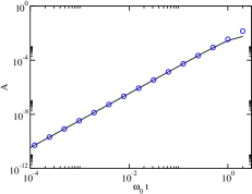
Figure 4: Color online. Function $A(t)$ as a function of the time elapsed between two Ramsey pulses (in units of $1/\omega_{0}$). The solid line corresponds to Eq. (37) and the symbols correspond to the short-time expansion in Eq. (40). The curve has been evaluated for $\eta^{(c)}=0.05$ in a linear chain of $N=10^{3}$ ions.

We now focus on the behaviour of the visibility for short elapsed times $t$. In this regime the autocorrelation function ${\mathcal{G}}(t)$, and correspondingly the logarithm of the visibility $A(t)$ in Eq. (37), can be expanded in powers of $\omega_{y}(k)t\ll 1$. At lowest order in the expansion one finds

$$A\simeq\Gamma t^{2}\,,$$ (40)

where

$$\Gamma = \frac{1}{2}\sum_{k,\sigma}|\alpha_{k\sigma}|^{2}\omega_{y}(k)^{2}\,,$$ (41)

and the condition $\omega_{\rm max}t\ll 1$ must hold. The correlation function hence goes quadratically with time, as shown in Fig. 4, and correspondingly the visibility signal decays with a Gaussian-type behaviour. In particular, for the linear chain the coefficient $\Gamma$ can be rewritten as

$$\Gamma=\frac{\hbar k_{L}^{2}}{4m}\left(\frac{1}{N}\sum_{k,\sigma}\omega_{y}(k)\right)\,,$$ (42)

and is hence proportional to the mean value of the frequency of the transverse excitations. The detailed derivation of this expression is reported in Appendix B. Equation (42) has been obtained for ions in a ring trap with large radius. It approximates well the result for a linear chain in a linear Paul trap when $N\gg 1$.

Figure 5: Color online. Coefficient $\Gamma$ (in units of $\omega_{0}^{2}$) as a function of $\Delta=\nu_{t}-\nu_{t}^{(c)}$ (in units of $\omega_{0}$). The solid line corresponds to the coefficient $\Gamma$, given in Eq. (41) and the symbols correspond to the value $\Gamma_{\rm fit}$, obtained by fitting the function $A(t)$ in Eq. (37) with the function $\Gamma_{\rm fit}t^{2}$. The parameters are the same as in Fig. 4. Inset: Derivative of $\Gamma$ with respect to $\Delta$ (in units of $\omega_{0}$) as a function of $\Delta$ (in units of $\omega_{0}$ and logarithmic scale) for $\Delta>0$ (symbols). An analytical analysis of the asymptotic behaviour, as well as a numerical fit of the curve give a logarithmic dependence of the derivative on $\Delta$ for $\Delta\to 0^{+}$ (line).

We now analyze the dependence of the coefficient $\Gamma$ on $\nu_{t}$ for values close to $\nu_{t}^{(c)}$, thereby getting further insight on the behaviour of the correlation function close to the critical point. Figure 5 displays $\Gamma$ as a function of $\Delta=\nu_{t}-\nu_{t}^{(c)}$ for values close to the value $\Delta=0$. One clearly observes a minimum, with a cusp-like behaviour, at the critical value $\nu_{t}^{(c)}$ corresponding to $\Delta=0$, showing that decay of the visibility signal as a function of the elapsed time is slowed down close to the critical point. The discontinuity of the derivative of $\Gamma$ with respect to $\Delta$ can be attributed to the structural phase transition that the chain undergoes at $\Delta=0$. In particular, an analytical study shows that for $\Delta>0$ (on the side of the linear chain) the derivative $d\Gamma/d\Delta\sim\ln\Delta$ as $\Delta\to 0^{+}$. This result, whose derivation is reported in Appendix B, is confirmed by a numerical fit, and is shown in the inset of Fig. 5.

As anticipated in Sec. II.3, analogous features have been found in the Loschmidt echo of a spin coupled to a quantum spin bath, when studying the short-time behaviour of the echo signal as a function of the control parameter close to the critical point of the spin chain (see in particular Figs. 2 and 3 of Ref. spin-rossini ).

IV.2 Long times: revivals and asymptotic value of the visibility

We finally investigate the behaviour of the visibility ${\mathcal{V}}(t)$ when long times $t$ are elapsed between the Ramsey pulses, focusing on values of the trap frequency $\nu_{t}$ close to the critical point. We consider time scales, such that the elapsed time satisfies the relation $\omega_{\rm min}t\gg 1$. While the asynchronous oscillations of the modes of the chain, excited by the photon recoil, lead to a decay of the visibility as a function of $t$, in finite systems we expect to observe characteristic elapsed times $t^{*}$ where a quasi-synchronization of the motion of the chain will occur, and, correspondingly, a sort of revival in the behaviour of the visibility signal is observed. The time $t^{*}$ can be estimated by considering the propagation speed at which the mechanical excitation propagates through the crystal and returns to the initial position. This corresponds to the approximated formula porras-spin-boson

$$t^{*}=\frac{Na}{v_{max}},$$ (43)

where $v_{max}=\max_{k}\partial\omega_{k}/\partial k$ is the maximum group velocity in the interval $k\in[0;\pi/a]$. Figure 6 displays the visibility signal as a function of the elapsed time for a linear chain composed by $N=10^{3}$ ions and close to the zigzag instability, $\Delta=10^{-3}\omega_{0}$. For $\eta^{(c)}=0.25$ the group velocity is maximum at $k=2.64/a$, taking the value $v_{max}=0.81a\omega_{0}$. Using this result, the estimated time from Eq. (43) is $t^{*}=1229/\omega_{0}$ which approximately coincides with the time at which the visibility exhibits sudden oscillations of larger amplitude.

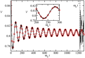
Figure 6: Color online. Behavior of the visibility signal for long times. The exact result for the visibility $\mathcal{V}$ (solid) obtained using Eqs. (36) and (37) and the approximate function $\exp[-\tilde{A}_{\infty}-\tilde{B}(t)]$ (symbols) (see Eqs. (47) and (48)) as a function of time (in units of $1/\omega_{0}$) for $\Delta=10^{-3}\omega_{0}$ (linear chain) with $N=10^{3}$ and $\eta^{(c)}=0.25$. The vertical dashed line corresponds to an estimate of the revival time according to the formula in Eq. (43), which gives $t^{*}=1229/\omega_{0}$. Inset: the same plot in a smaller region for a closer comparison between $\mathcal{V}$ and the approximated expression $\exp[-\tilde{A}_{\infty}-\tilde{B}(t)]$.

We now focus on the regime, in which the system is sufficiently large, $N\gg 1$, and derive the asymptotic form of the visibility signal for times $t\to\infty$, obtained by averaging over time intervals $T\gg t^{*}$. The asymptotic form of ${\mathcal{V}}(t)$ of can be singled by observing that the exponent $A(t)$ in Eq. (38) can be rewritten as

$$A=A_{\infty}+B(t)$$ (44)

where

$$A_{\infty} = \frac{k_{L}^{2}}{2}\left[\langle y_{1}^{2}(t)\rangle+\langle y_{1}^{2}(0)\rangle\right]=\sum_{k\sigma}|\alpha_{k\sigma}|^{2}\,,$$ (45)

$$B(t) = k_{L}^{2}{\rm Re}\langle y_{1}(t)y_{1}(0)\rangle=\sum_{k\sigma}|\alpha_{k\sigma}|^{2}\cos\omega_{y}(k)t\,.$$ (46)

Using Eq. (38) we see that $A_{\infty}$ is proportional to the variance of the ion displacement $\langle y_{1}^{2}(t)\rangle=\langle y_{1}^{2}(0)\rangle$ around its equilibrium position, while $B(t)$ is proportional to the real part of the crystal’s correlation function $\langle y(t)y(0)\rangle$.

For $N\gg 1$, and when the linear chain is close to the instability, $\Delta\to 0^{+}$, Eqs. (45) and (46) can be approximated by the quantities

$$A_{\infty} \simeq \tilde{A}_{\infty}=-\frac{\eta_{0}^{2}\nu_{t}a}{2\pi h}\ln\Delta+c,$$ (47)

$$B(t) \simeq \tilde{B}(t)=-\frac{\eta_{0}^{2}\nu_{t}a}{2h}N_{0}(\delta t),$$ (48)

where $c$ is a constant, $N_{0}$ is the Bessel function of the second kind (see Appendix B) and we introduced the parameters $h=\sqrt{\ln 2}~{}\omega_{0}a$ and

$$\delta=\sqrt{\nu_{t}^{2}-\nu_{t}^{(c)2}},$$ (49)

which is related to the parameter $\Delta$ by the relation $\delta=\sqrt{\Delta(2\nu_{t}^{(c)}+\Delta)}$. In Fig. 6 we compare the exact result of the visibility with the approximated function $\tilde{\mathcal{V}}(t)=\exp[-\tilde{A}_{\infty}-\tilde{B}(t)]$. For long times, such that $t\gg 1/\delta$, the function $B(t)$, and as a result the two-time correlation function of the crystal, decays as $1/\sqrt{\delta t}$ and the visibility approaches the asymptotic value given by $V_{\infty}=\exp[-A_{\infty}]$. Figure 7 displays $A_{\infty}$ as a function of $\Delta$, showing that $A_{\infty}$ (and therefore the spatial width of the ion wavepacket) diverges logarithmically with $\nu_{t}$ close to the critical point. As a consequence, the asymptotic value of the visibility $\mathcal{V}_{\infty}$ becomes smaller when the ion chain is close to the mechanical instability, where it undergoes a second-order phase transition to the zigzag structure. This behavior of the visibility is qualitatively similar to the behavior of the asymptotic Loschmidt echo $\mathcal{L}_{\infty}$ for a spin interacting with an Ising chain close to the critical magnetic field spin-rossini .

Figure 7: The asymptotic value of the correlation function, as given by $A_{\infty}$ in Eq. (45), as a function of $\Delta$ when the linear chain is close to the critical point, where it makes a transition to the zigzag structure. The symbols correspond to the curve given by Eq. (45) and the solid line is the curve obtained from the analytical prediction in Eq. (47). The parameters are $N=10^{3}$ and $\eta^{(c)}\simeq 0.05$.

V Conclusions

The aim of this work was to understand the dynamical properties of a quasi-one-dimensional many-body system externally driven and probed via one of its components, in a setup that is both experimentally feasible and not previously studied in this context – a chain of trapped ions. The ions form a Coulomb crystal undergoing a second-order phase transition between a linear and a zig-zag configuration, depending on the transverse trapping strength. Building on interferometric methods with trapped ions Sackett , we proposed a Ramsey experiment to measure the autocorrelation function of an ion crystal by only exciting and detecting the internal state of one of its constituent ions.

The central quantity to this study is the visibility of the fringes of this specific implementation of the Ramsey interferometer. We show that it provides information of the dynamical and statistical properties of the crystal. In particular, for the specific realization here proposed the visibility allows one to measure the autocorrelation function of the crystal, and the characteristic decay time, thereby accessing its properties close to the critical point.

It is interesting to remark that several features of the Ramsey signal, close to the critical point where the linear chain undergoes a transition to a zig-zag configuration, share several analogies with the Loschmidt echo evaluated for studying the decoherence of a spin coupled to quantum spin-baths close to criticality spin-rossini ; paganelli ; spin-zanardi ; cucchietti . In fact, the crystal can be regarded as a reservoir with respect to the single spin constituted by the two internal states of the probed ion. In this sense our system can be seen as a model for decoherence induced by a bath at $T=0$. On the other hand, a distinguishing feature of our proposal is the presence of long-range interactions, typically absent in (nearest-neighbor interacting) spin systems.

We conclude by observing that the ability to drive and probe the whole crystal by addressing just one ion opens interesting questions like the possibility of using the methods developed here to identify control procedures, of spin-echo type, to maintain coherence in the system, as well as to measure other quantities, such as, e.g., coherence length and quantum fluctuations at a quantum critical point. This points to the need for a thorough understanding of quantum phase transitions in ion traps, as initiated in retzker . The adaptation and further development of the ideas proposed here to the latter context will be the subject of our future work.

Appendix A

In this appendix we provide more details on the eigenmodes of the linear and zigzag structures. A more extensive treatment can be found in fishman2008 . For a linear ion chain in a harmonic trap, the reader is referred to morigi2004 .

Linear chain. For a given frequency $\omega_{x}(k)$, $\omega_{y}(k)$ there are in general two modes of opposite parity with respect to the transformation $q_{j}\to q_{-j}$, $y_{j}\to y_{-j}$, even $\sigma=+$ and odd $\sigma=-$. The frequencies at wave vectors $k=0$ and $k=\pi/a$ are instead not degenerate. The corresponding modes are the bulk and the zigzag mode, respectively, which have definite parity, the first being even and the latter odd. For the transverse excitations, the bulk mode is at frequency $\nu_{t}$ while the zigzag mode is at frequency $\omega_{y}(k=\pi/a)$. For the modes at wave vector $0<k<\pi/a$, the elements of the orthogonal matrix, connecting the displacements of the ions from the equilibrium positions with the eigenmodes amplitudes, read

$${\cal R}_{j,k+} = \sqrt{\frac{2}{N}}\cos(jka)\,,$$ (50)

$${\cal R}_{j,k-} = \sqrt{\frac{2}{N}}\sin(jka)\,,$$ (51)

while the elements connecting the displacements from the equilibrium positions with the bulk and zigzag eigenmodes take the form

$${\cal R}_{j,0} = \sqrt{\frac{1}{N}}\,,$$ (52)

$${\cal R}_{j,\frac{\pi}{a}} = (-1)^{j}\sqrt{\frac{1}{N}}\,.$$ (53)

Zigzag configuration. In the zigzag structure the dispersion relation is now defined in the Brillouin zone $[0,\pi/2a]$, such that the wave vector $k$ takes the values $k=2\pi n/Na$ with $n=0,\ldots,N/4$. As shown in fishman2008 the spectrum of excitations consists of four branches that we label $\beta=1,2,3,4$. For a given frequency $\omega_{\beta}^{zz}(k)$ for $0<k<\pi/2a$ there are two modes with opposite parities $\sigma=\pm$ which are a combination of displacements in the longitudinal and transverse directions. The correspondent elements of the matrix ${\cal R}^{zz}$ read

$${\cal R}^{zz}_{2j-1,k\beta+} = u_{\beta}\cos(\tilde{k}aj)\,,$$ (54)

$${\cal R}^{zz}_{2j,k\beta+} = v_{\beta}\sin[(\pi-\tilde{k}a)j]\,,$$ (55)

$${\cal R}^{zz}_{2j-1,k\beta-} = u_{\beta}\sin[\tilde{k}aj]\,,$$ (56)

$${\cal R}^{zz}_{2j,k\beta-} = -v_{\beta}\cos[(\pi-\tilde{k}a)j]\,,$$ (57)

with $j=1,2,\dots,N$ labeling the ion displacements $\varrho_{2j-1}=q_{j}$ and $\varrho_{2j}=w_{j}$; and $\tilde{k}=k$ for $\beta=1,2$, $\tilde{k}=\pi/a-k$ for $\beta=3,4$. The explicit form of the coefficients $u_{\beta}$ and $v_{\beta}$ can be found in fishman2008 (check Eq. (20)).

For $k=0$ the normal modes are the bulk modes in the $x$ and $y$ directions. These modes correspond to the zigzag structure oscillating rigidly in the $x$ or $y$ directions. The matrix elements for the bulk mode in the $x$ direction are:

$${\cal R}^{zz}_{2j-1,0x}=\sqrt{\frac{1}{N}};\quad{\cal R}^{zz}_{2j,0x}=0;$$ (58)

while for the bulk mode in the $y$ direction they are

$${\cal R}^{zz}_{2j-1,0y}=0;\quad{\cal R}^{zz}_{2j,0y}=\sqrt{\frac{1}{N}}.$$ (59)

For $k=\pi/2a$ the normal modes are the two zigzag modes along the $x$ and $y$ direction. The zigzag mode in the $x$ direction is the mode where neighboring ions oscillate around the equilibrium positions along the $x$ axis and with opposite phase. The corresponding matrix elements are given by:

$${\cal R}^{zz}_{2j-1,\frac{\pi}{2a}\,x}=(-1)^{j}\sqrt{\frac{1}{N}};\quad{\cal R}^{zz}_{2j,\frac{\pi}{2a}\,x}=0.$$ (60)

Analogously, for the zigzag mode in the $y$ direction, the matrix elements are:

$${\cal R}^{zz}_{2j-1,\frac{\pi}{2a}\,y}=0;\quad{\cal R}^{zz}_{2j,\frac{\pi}{2a}\,y}=(-1)^{j}\sqrt{\frac{1}{N}}.$$ (61)

Appendix B

In this section we determine analytically the behaviour of the function $A(t)$, Eq. (37), for short and long elapsed times $t$. We focus on the linear chain, when the parameters are such that $\nu_{t}$ is close to the value $\nu_{t}^{(c)}$ of the transition to the zigzag configuration.

Short time behaviour. For short times, such that $\nu_{t}t\ll 1$, we expand $A(t)$ at lowest order in the small parameter $\omega_{y}(k)t\ll 1$, obtaining Eq. (40), where $\Gamma$ is given by expression (41). In the linear chain ($\Delta>0$), using the definition of $\alpha_{k\sigma}$ in Eq. (28) with the corresponding values of the elements of the matrix ${\cal R}$ in Eqs. (50)-(53), we find

$$\Gamma = \frac{\hbar k_{L}^{2}}{4m}\sum_{k,\sigma}\mathcal{R}_{1,k\sigma}^{2}\omega_{y}(k)=$$ (62)

$$= \frac{\hbar k_{L}^{2}}{4m}\left(\frac{1}{N}\sum_{k,\sigma}\omega_{y}(k)\right)\,.$$ (63)

The value of $\Gamma$ is hence proportional to the mean value of the transverse frequencies.

An explicit form of the mean value can be obtained close to the phase transition, when $\Delta=\nu_{t}-\nu_{t}^{(c)}\ll\nu_{t}^{(c)}$, and for a sufficiently large number of ions. In this limit, we can approximate the dispersion relation Eq. (18) for small momenta $q=\pi/a-k$ as:

$$\omega_{y}(q)\simeq\sqrt{\delta^{2}+h^{2}q^{2}}\,,$$ (64)

where $\delta=\sqrt{\nu_{t}^{2}-\nu_{t}^{(c)2}}\simeq\sqrt{2\nu_{t}^{(c)}\Delta}$ and $h=\sqrt{\ln 2}\omega_{0}a$. Taking the continuum limit in Eq. (63) we find

$$\Gamma \simeq \frac{1}{2}\eta_{0}^{2}\nu_{t}\frac{a}{\pi}\int_{0}^{\pi/a}dk\omega_{y}(k)$$ (65)

$$\simeq \frac{1}{2}\eta^{2}_{0}\nu_{t}\frac{a}{\pi}\int_{0}^{q_{\rm max}}\sqrt{\delta^{2}+h^{2}q^{2}}dq+c$$

$$= \frac{1}{4}\eta^{2}_{0}\nu_{t}\frac{a}{\pi}\frac{1}{h}\left[hq_{\rm max}\sqrt{\delta^{2}+h^{2}q_{\rm max}^{2}}+\right.$$

$$+ \left.\delta^{2}\textrm{arcsinh}\left(\frac{hq_{\rm max}}{\delta}\right)\right]+c\,,$$

where $q_{\rm max}$ is a cutoff and $c$ is a constant which depends on the cutoff. The derivative of $\Gamma$ with respect to $\Delta$, for $\Delta\to 0^{+}$ is obtained from Eq. (65) and reads

$$\frac{d\Gamma}{d\Delta}=-\frac{1}{4}\eta^{2}_{0}\nu_{t}\frac{\nu_{t}^{(c)}a}{\pi h}\ln\Delta+c_{1}\,,$$ (66)

where $c_{1}$ depends on $q_{\rm max}$ and and we neglected terms which goes to zero as $\Delta\to 0$.

Long time behaviour. We now study the behaviour of the function $A(t)$ for long times. The quantity $A_{\infty}$ can be cast in a simplified form for the linear chain. Using the same technique which leads to Eq. (63), one finds

$$A_{\infty}=\frac{\hbar k_{L}^{2}}{2m}\left(\frac{1}{N}\sum_{k,\sigma}\frac{1}{\omega_{y}(k)}\right)\,.$$ (67)

The value close to the critical point and for large chains can be found following the same procedure applied for obtaining Eq. (65). We get

$$A_{\infty} \simeq \frac{\hbar k_{L}^{2}}{2m}\frac{a}{\pi}\int_{0}^{q_{\rm max}}\frac{dq}{\sqrt{\delta^{2}+h^{2}q^{2}}}$$ (68)

$$\simeq -\frac{\eta_{0}^{2}\nu_{t}a}{2\pi h}\ln\Delta+c\,,$$

where $c$ is a constant which depends on $q_{\rm max}$ and we omitted terms which vanish when $\delta\to 0$. We now turn to the expression (46) for $B(t)$ and with the aid of formula (64) we can approximate it as:

$$B(t) = \frac{\eta_{0}^{2}\nu_{t}a}{\pi}\int_{0}^{\infty}\frac{\cos\omega_{y}(q)t}{\omega_{y}(q)}dq$$ (69)

$$= -\frac{\eta_{0}^{2}\nu_{t}a}{2h}N_{0}(\delta t)\,,$$ (70)

where we let $q_{\rm max}\to\infty$. The function $N_{0}(x)$ is the Bessel function of the second kind (also von Neumann function) grad . At the asymptotics, for $x\to\infty$, it behaves as grad

$$N_{0}(x)\simeq\frac{\sin x-\cos x}{\sqrt{\pi x}}\,,$$ (71)

and hence vanishes as $1/\sqrt{x}$.

References

- (1) P. Zoller et al., Quantum information processing and communication, Eur. Phys. J. D 36, 203 (2005).
- (2) W. H. Zurek, Phys. Today 44, 36 (1991).
- (3) G.W. Ford, M. Kac, and P. Mazur, Jour. Math. Phys. 6, 504 (1965).
- (4) A. J. Leggett, S. Chakravarty, A. T. Dorsey, M. P. A. Fisher, A. Garg, and W. Zwerger, Rev. Mod. Phys. 59, 1 (1987).
- (5) U. Weiss, Quantum Dissipative Systems, World Scientific (Singapore, 1999).
- (6) D.H.E. Dubin and T.M. O’Neil, Rev. Mod. Phys. 71, 87 (1999).
- (7) J.I. Cirac, P. Zoller, Phys. Rev. Lett. 74, 4091 (1995).
- (8) F. Schmidt-Kaler, H. Häffner, M. Riebe, S. Gulde, G. P. T. Lancaster, T. Deuschle, C. Becher, C. F. Roos, J. Eschner, and R. Blatt, Nature 422, 408 (2003); D. Leibfried, B. DeMarco, V. Meyer, D. Lucas, M. Barrett, J. Britton, W. M. Itano, B. Jelenkovic, C. Langer, T. Rosenband, and D. J. Wineland, Nature 422, 412 (2003). M.J. McDonnell, J.P. Home, D.M. Lucas, G. Imreh, B.C. Keitch, D.J. Szwer, N.R. Thomas, S.C. Webster, D.N. Stacey, and A.M. Steane, Phys. Rev. Lett. 98, 063603 (2007); J. Benhelm, G. Kirchmair, C. F. Roos, R. Blatt, Nature Physics 4, 463 (2008).
- (9) F. Mintert and C. Wunderlich, Phys. Rev. Lett. 87, 257904 (2001).
- (10) D. Porras and J. I. Cirac, Phys. Rev. Lett. 92, 207901 (2004); D. Porras and J.I. Cirac, Phys. Rev. Lett. 96, 250501 (2006).
- (11) D. Porras, F. Marquardt, J. von Delft, and J. I. Cirac, preprint arXiv:0710.5145 (2007).
- (12) A. Friedenauer, H. Schmitz, J.T. Glückert, Diego Porras, Tobias Schätz, preprint arXiv:0802.4072 (2008).
- (13) N. Kjargaard and M. Drewsen, Phys. Rev. Lett. 91, 095002 (2003); A. Mortensen, E. Nielsen, T. Matthey, and M. Drewsen, Phys. Rev. Lett. 96, 103001 (2006).
- (14) W. M. Itano, J. J. Bollinger, J. N. Tan, B. Jelenkovic, X. P. Huang, and D. J. Wineland, Science 279, 686 (1998).
- (15) M Block, A Drakoudis, H Leuthner, P Seibert, G Werth, M Block, A Drakoudis, H Leuthner and P Seibert J. Phys. B: At. Mol. Opt. Phys. 33, L375 (2000).
- (16) P.K. Ghosh, Ion Traps (Clarendon, Oxford, 1995).
- (17) G. Birkl, S. Kassner, H. Walther, Nature 357, 310 (1992); I. Waki, S. Kassner, G. Birkl, and H. Walther, Phys. Rev. Lett. 68, 2007 (1992).
- (18) M.G. Raizen, J.M. Gilligan, J.C. Bergquist, W.M. Itano, and D.J. Wineland, Phys. Rev. A 45, 6493 (1992).
- (19) D.H.E. Dubin, Phys. Rev. E 55, 4017 (1997).
- (20) G. Piacente, I. V. Schweigert, J. J. Betouras, and F. M. Peeters, Phys. Rev. B 69, 045324 (2004).
- (21) G. Morigi and S. Fishman, Phys. Rev. Lett. 93, 170602 (2004); G. Morigi and S. Fishman, Phys. Rev. E 70, 066141 (2004).
- (22) D.H.E. Dubin, Phys. Rev. Lett. 71, 2753 (1993). See also J.P. Schiffer, Phys. Rev. Lett. 70, 818 (1993).
- (23) S. Fishman, G. De Chiara, T. Calarco, and G. Morigi, Phys. Rev. B 77, 064111 (2008).
- (24) H.J. Schulz, Phys. Rev. Lett. 71, 1864 (1993).
- (25) J. Yin and J. Javanainen, Phys. Rev. A 51, 3959 (1995).
- (26) A. Retzker, R. Thompson, D. Segal, and M.B. Plenio, arXiv:0801.0623.
- (27) D. Leibfried, D.M. Meekhof, B.E. King, C. Monroe, W.M. Itano, and D.J. Wineland, Phys. Rev. Lett. 77, 4281 (1996);
- (28) D. Leibfried, E. Knill, S. Seidelin, J. Britton, R. B. Blakestad, J. Chiaverini, D. B. Hume, W. M. Itano, J. D. Jost, C. Langer, R. Ozeri, R. Reichle, and D. J. Wineland, Nature 438, 639 (2005); H. Häffner, W. Hänsel, C. F. Roos, J. Benhelm, D. Chek-al-kar, M. Chwalla, T. Körber, U.D. Rapol, M. Riebe, P.O. Schmidt, C. Becher, O. Gühne, W. Dür and R. Blatt, Nature 438, 643 (2005).
- (29) N. Ramsey, Molecular Beams (Oxford Univ. Press, Oxford, UK, 1985).
- (30) J. F. Poyatos, J. I. Cirac, R. Blatt, and P. Zoller, Phys. Rev. A 54, 1532 (1996).
- (31) P. Bertet, S. Osnaghi, A. Rauschenbeutel, G. Nogues, A. Auffeves, M. Brune, J. M. Raimond and S. Haroche, Nature 411, 166 (2001).
- (32) C.J. Myatt, B.E. King, Q.A. Turchette, C.A. Sackett, D. Kielpinski, W.M. Itano, C. Monroe, and D.J. Wineland, Nature (London) 403, 269 (2000); Q.A. Turchette, C.J. Myatt, B.E. King, C.A. Sackett, D. Kielpinski, W.M. Itano, C. Monroe, and D.J. Wineland, Phys. Rev. A 62, 053807 (2000)
- (33) J. P. Paz and W. H. Zurek, in Coherent matter waves, Les Houches Session LXXII, R Kaiser, C Westbrook and F David eds., EDP Sciences (Springer Verlag, Berlin, 2001), pp. 533-614.
- (34) A. Polkovnikov, E. Altman, and E. Demler, PNAS 103, 6125 (2006); S. Hofferberth, I. Lesanovsky, T. Schumm, J. Schmiedmayer, A. Imambekov, V. Gritsev, E. Demler, Nature Physics 4, 489(2008).
- (35) J. Eschner, G. Morigi, F. Schmidt-Kaler, and R. Blatt, J. Opt. Soc. Am. B 20, 1003 (2003).
- (36) B.-G. Englert, Phys. Rev. Lett. 77, 2154 (1996).
- (37) F.M. Cucchietti, D.A.R. Dalvit, J.P. Paz and W.H. Zurek, Phys. Rev. Lett. 91, 210403 (2003).
- (38) D. Rossini, T. Calarco, V. Giovannetti, S. Montangero and R. Fazio, J. Phys. A: Math. Theor. 40, 8033 (2007); Phys. Rev. A 75, 032333 (2007).
- (39) G. Morigi and S. Fishman, J. Phys. B 39, S221 (2006).
- (40) N.W. Ashcroft and N.D. Mermin, Solid State Physics (Saunders College, Philadelphia, 1976).
- (41) G. Morigi and H. Walther, Eur. Phys. Jour. D 13, 261 (2001); See also Eur. Phys. Jour. D 15, 137 (2001).
- (42) G. Morigi and J. Eschner, Phys. Rev. A 64, 063407(2001).
- (43) S. Paganelli, F. de Pasquale, and S.M. Giampaolo, Phys. Rev. A 66, 052317 (2002).
- (44) H.T. Quan, Z. Song, X.F. Liu, P. Zanardi and C.P. Sun, Phys. Rev. Lett. 96, 140604 (2006).
- (45) F.M. Cucchietti, S. Fernandez-Vidal and J.P. Paz, Phys. Rev. A 75, 032337 (2007).
- (46) Table of integrals, series, and products, edited by I. S. Gradshteyn and I.M. Ryzhik (Academic Press, New York, 1981).