Intelligent tit-for-tat in the iterated prisoner’s dilemma game

Abstract

We seek a route to the equilibrium where all the agents cooperate in the iterated prisoner’s dilemma game on a two-dimensional plane, focusing on the role of tit-for-tat strategy. When a time horizon, within which a strategy can recall the past, is one time step, an equilibrium can be achieved as cooperating strategies dominate the whole population via proliferation of tit-for-tat. Extending the time horizon, we filter out poor strategies by simplified replicator dynamics and observe a similar evolutionary pattern to reach the cooperating equilibrium. In particular, the rise of a modified tit-for-tat strategy plays a central role, which implies how a robust strategy is adopted when provided with an enhanced memory capacity.

I Introduction

One of the main interests in statistical physics is related with the equilibration process of a given system composed of many interacting elements. For instance, the classical Ising system made up of locally interacting spins approaches an equilibrium, characterized by the minimum of the Helmholtz free energy. Such a model system in statistical physics is defined by the Hamiltonian and can be readily studied by updating spins with local Monte Carlo rules in numerical simulations Newman . A lot of interactions including ecological, social, and economical ones are more complicated than that of spins as they are usually asymmetric and history dependent. Furthermore, most of these systems beyond the simple physics model cannot be described by the simple Hamiltonian approach. Even if no analytical solution is available, we may expect the system to evolve by successive local adaptations, with searching for an optimal point on the fitness landscape. However, when the interaction is asymmetric, it is possible that the equilibrium reached by local dynamics may not be optimal in a global sense.

The prisoner’s dilemma (PD) game is a famous model of such disparity. The typical story begins as follows. Two suspected accomplices are caught by the police for a crime deserving of 4 years’ imprisonment each. After separating two suspects from each other, the police offers a deal to each of them: If only one confesses the crime and the other remains silent, the informer will be rewarded and set free, while the other one will receive an aggravated punishment (say 5 years in prison). On the other hand, if both keep silent, they will get some punishment which is supposed to be not so heavy (e.g., 2 years in prison). It is still true that they can get light punishments by cooperating to each other. From an individual viewpoint, however, it is always better to defect the other, so they will be eventually sentenced 8 years in total as the police wanted. Throughout the present paper, the game results are quantified by four elementary payoffs: The temptation to defect as $T=5$, the reward of cooperation as $R=3$, the punishment from mutual defection as $P=1$, and the damage from being sucked as $S=0$. Note that the payoffs satisfy two inequalities. The first one $T>R>P>S$ locates the Nash equilibrium Nash at mutual defection, and the second $2R>T+S$ sets the mutual cooperation as optimal in total.

The conclusion of the PD game is highly nontrivial in that local optimization will end up with the poorest result in a global sense. The first breakthrough in this dilemma was made by performing the game iteratively, where the system could achieve the optimal point of mutual cooperation Axelrod . Iteration affects the system’s trajectory in two ways: Since the strategy space comes to have a much larger dimensionality than choosing between cooperation and defection, there enters a possible route to mutual cooperation. In addition, as the time scale of interaction is separated from that of selection, the stability of equilibria and their basins of attraction may be changed: As to the PD game, for example, slow selection favors the weaker strategy (i.e., cooperation) from a population genetics point of view Roca . Nevertheless, the equilibrium in which all agents cooperate is usually accessed by a detour consisting of intermediate stages.

In the iterated PD game, there are successfully cooperating strategies some of which are as follows: (i) Grim trigger (GT) initially cooperates, but any single defection by its opponent makes GT defect forever Friedman . (ii) tit-for-tat (TFT) also starts with cooperation, and then does what the opponent did. This simple strategy is famous for its own virtues, i.e., being nice, retaliating, forgiving, and nonenvious Axelrod . By nice, we mean that a strategy never provokes the opponent first by defection. Likewise, retaliating and forgiving mean that it defects after defected, and cooperates when the opponent changes back to cooperation. Finally, by being nonenvious, TFT allows coexistence of other strategies. However, one should note that an erroneous defection between TFT’s leads to a chain retribution until a new error makes them cooperate again. (iii) Pavlov keeps its last move if paid highly and switches to a different move otherwise, as it is often called win-stay lose-shift Kraines . Unlike the other two, it forgives a mistake between themselves.

Since the above-mentioned three strategies remember only the moves in the last time step, they all belong to a set of strategies which are confined in the time horizon of one time step, which we will call $M_{1}$. Note that the actual amount of information in use is different: GT and TFT require only the opponent’s last move, while Pavlov recalls both of its opponent’s and its own. Likewise, $M_{n}$ means the set of strategies which uses the last $k(\leq n)$ time steps in making a decision. By giving an explicit restriction to the time horizon, our strategy space is different from that in the state space approach Leimar .

In order to investigate how the system is evolved by selection and adaptation, we start with every possible strategy in $M_{1}$ and $M_{2}$, respectively, and examine surviving strategies to understand the route to the equilibrium. While the genetic algorithm has been often used in exploring a large strategy space Axelrod1987 ; Miller , we aim at an almost exhaustive search in that all the strategies are explicitly considered at least once. In particular, we do not include any mutation processes as in Ref. Lindgren1994 for fixing the strategy space we must scan. Nor do we treat stochastic strategies Nowak1990 ; Nowak1992a ; Nowak1993 ; Hauert , as the deterministic representation shows the pure decision characteristics of a strategy more clearly. Note that we mostly employ typical setups except for the time horizon in order to keep the situation as simple as possible. We therefore pass over many interesting variations of the PD game, such as the idea of payoff-based strategies killing . The spatial structure we study here is a two-dimensional plane which provides spatial reciprocity for cooperators spatial (see, e.g., Refs. network ; szabo for other topological structures), but we do not employ the dynamic preferential selection sheng and let each agent play with its every neighbor equally. Under such conditions, we find that $M_{2}$ has its own TFT modified from the original one in $M_{1}$, which seemingly indicates a generic pattern in the evolution of cooperation. Even though the reciprocity has been thought of as relevant to the emergence of cooperation even in longer time horizons Axelrod1987 , such concrete strategic forms, which are directly related to the original TFT, have not been reported yet.

The present paper is organized as follows: In Sec. II, we check the case of $M_{1}$ to introduce our basic scheme. In Sec. III, we apply it to $M_{2}$ and present the surviving strategies, including the modified type of TFT. Finally, we discuss and conclude this work in Sec. IV.

II Methods

II.1 Bitwise representation of strategies in $M_{1}$

A strategy in $M_{1}$ can be conveniently denoted by five bits, each of which can take either cooperation ($C$) or defection ($D$): The first bit, $\alpha$, is the move when a player first encounters an opponent and thus has empty memory. The bit $a_{1}$ is the move at time $t$ when the player’s and opponent’s previous moves at $t-1$ were $C$ and $C$ [henceforth we denote this situation as (player’s move at $t-1$, opponent’s move at $t-1$) = $(C,C)$] , respectively (Table 1). Likewise, $a_{2}$ is for $(C,D)$, $a_{3}$ for $(D,C)$, and $a_{4}$ for $(D,D)$.

Table 1: Bitwise representation of a strategy in $M_{1}$ as $\alpha|a_{1}a_{2}a_{3}a_{4}$.

State	Empty	($C$,$C$)	($C$,$D$)	($D$,$C$)	($D$,$D$)
Player’s move	$\alpha$	$a_{1}$	$a_{2}$	$a_{3}$	$a_{4}$

Consequently, a strategy in $M_{1}$ is coded by $\alpha|a_{1}a_{2}a_{3}a_{4}$ and the total number of strategies is $|M_{1}|=2^{5}=32$, for each of five bits can have either $C$ or $D$. For example, $C|CDDD$, $C|CDCD$, and $C|CDDC$ encode GT, TFT and Pavlov, respectively. Further examples include the unconditional cooperator (ALLC or AC) coded by $C|CCCC$ and the unconditional defector (ALLD or AD) by $D|DDDD$. A nice strategy (see above) in $M_{1}$ is represented as $\alpha=C$, implying that it starts with $C$ at the first encounter, and $a_{1}=C$, meaning that it never provokes the defection first .

II.2 Transition graphs and tournament for $M_{1}$

Another way of representing a strategy is to mention all of the possible states it may meet and all of the possible transitions between them Miller ; Ashlock ; Sethi . Identifying each state with a vertex and each transition with an arc (a directed edge), with self-connecting included, this procedure yields a transition graph for each strategy. Suppose, for example, that Alice employs TFT and Bob does another arbitrary strategy in $M_{1}$. From Alice’s viewpoint, the four possible states are represented by four pairs; $(C,C)$, $(C,D)$, $(D,C)$, and $(D,D)$ where the former character indicates her last move and the latter does Bob’s. If starting with $(C,C)$, the next state must be $(C,X)$ with $X=C$ or $D$ depending on Bob’s strategy, because Alice remembers what Bob did at the last encounter. Repeating this for all the states gives Fig. 1. One can easily get the graphical representations for any other strategies by the same procedure, noting that the initial bit $\alpha$ does not change the transition graph but only makes the starting vertex in the graph different.

Figure 1: Transition graph for TFT. Each vertex represents a state in Table 1, and the directed edges are the possible next states allowed by this strategy. Each vertex has two outgoing arcs, considering the move taken by the opponent.

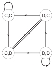
From all the 16 transition graphs in $M_{1}$, TFT is found to be unique in that it does not permit returning to $(C,D)$ without visiting $(D,C)$, which implies that any strategy cannot repeatedly suck TFT avoiding retaliation. In order to describe the time course of the PD game between two agents, the distinction between transient and recurrent states needs to be made: Transient states have only outward arcs and thus cannot be visited repeatedly, while the recurrent states are visited over and over again. For example, TFT does not have transient states, while AD has two transient states $(C,C)$ and $(C,D)$ with two recurrent states $(D,C)$ and $(D,D)$.

Figure 2: Transition graphs from combining two strategies in $M_{1}$. (a) GT vs GT. If deviated from $(C,C)$, the only attractor is mutual defection. (b) TFT vs TFT. If mistaken, they do not recover mutual cooperation on their own, unless another error brings them back. (c) Pavlov vs Pavlov, forgiving an error between themselves. (d) Pavlov vs GT. Pavlov is defeated by GT if any error occurs.

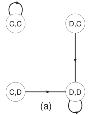
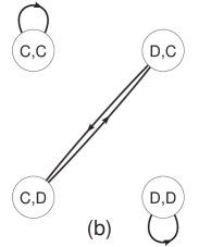
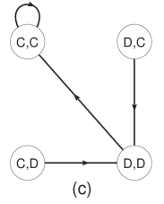
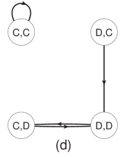
If two strategies $i$ and $j$ in $M_{1}$ play the PD game together, two corresponding graphs are combined to make one deterministic transition graph (Fig. 2). The move sequence is periodic and the long-time limit of the average payoff per time step is determined only by recurrent states of the two, from which one can calculate easily $U_{ij}$, the average payoff per step that the strategy $i$ gains from $j$. In the same spirit as the original tournament held by Axelrod, we compute the average points the strategy $i$ gets from all strategies (including $i$) to obtain Table 2. So far as each pair of strategies has an equal acquaintance probability, the tournament results will converge to these values in the long-time limit. Moreover, since each value in this table is analytically calculated from periodic moves in pairs of deterministic strategies, one can decompose it into the elementary payoffs, $T$, $R$, $P$, and $S$. For example, AD, AC, and GT earn $(T+P)/2=3$, $(R+S)/2=1.5$, and $R/2+(T+P)/4=3$, respectively. One can see that TFT is not the best within $M_{1}$ and that strategies with more $D$ bits often outperform cooperators. We emphasize that the above results in a round-robin tournament are not related to an evolutionary process yet and need to be checked from evolutionary perspectives.

Table 2: Average points $\frac{1}{|M_{1}|}\sum_{j}U_{ij}$ for each strategy in $M_{1}$.

Strategy	Points	Strategy	Points	Strategy	Points	Strategy	Points
AD	3.00	$C|DDDC$	2.73	$C|DDCC$	2.25	$C|DCCD$	1.69
$D|CCDD$	3.00	$D|DCDC$	2.73	$D|DDCD$	2.22	$C|DCCC$	1.63
$C|DDDD$	3.00	Pavlov	2.56	$C|CDCC$	2.19	AC	1.50
GT	3.00	$D|CCDC$	2.38	$D|CDCC$	2.09	$C|CCDC$	1.50
$D|CDDD$	3.00	$C|DDCD$	2.36	$D|CDCD$	2.02	$C|CCCD$	1.50
$D|DCDD$	3.00	TFT	2.35	$C|DCDC$	1.90	$C|CCDD$	1.50
$D|DDDC$	2.97	$D|DDCC$	2.25	$D|DCCD$	1.86	$D|CCCC$	1.50
$D|CDDC$	2.89	$C|DCDD$	2.25	$D|DCCC$	1.81	$D|CCCD$	1.38

II.3 Spatial prisoner’s dilemma game for $M_{1}$

The spatial PD game (SPDG) provides a good framework for observing the emergent cooperation as it allows the cooperating strategies to make clusters against defectors spatial . There is no unique standard in constructing SPDG, and a different rule may yield a different output, in general. Here we present our SPDG rules, which have been extensively used in literature szabo .

We perform SPDG on a two-dimensional $128\times 128$ square lattice with the periodic boundary condition. In the initial stage of the SPDG, one among all 32 strategies in $M_{1}$ is randomly assigned to each node of the lattice, and every agent plays the PD game with her four nearest neighbors. After all agents play the game, often called one Monte Carlo (MC) step, this procedure is stopped with a preassigned probability $p$ or repeats itself with $1-p$. When stopped, the sequence of games so far is termed as one generation whose average time duration is $1/p$ MC steps. In order to make the effects of transient states (see above) as weak as possible, $p$ should be sufficiently small to ensure that one generation is long enough (we observe that $p=0.05$, corresponding to one generation as 20 MC steps on average, fulfills this requirement). Whenever a generation is closed, the selection mechanism is activated as follows: Every node, one by one, randomly chooses one of its nearest neighbors and adopts the neighbor’s strategy if the neighbor has gained more during that generation. Memory tables for all pairs of agents are recalculated and payoffs are initialized back to zero, and then the next generation begins.

Figure 3: (Color online) Comparison between SPDG and RD. (a) A simulation result on a $128\times 128$ lattice with $p=0.05$. (b) Numerical integration of Eq. (2).

Figure 4: (Color online) A pattern in SPDG on the $128\times 128$ lattice with $e=0.01$ and $p=0.05$. Even with the presence of error, almost all the dynamical patterns at large time scales occur within the strategies found in the error-free RD, if the error probability is sufficiently low.

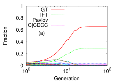
Our SPDG simulation readily shows that a cooperating equilibrium, in which all of the agents are playing $C$, is achieved mostly by GT, TFT, and Pavlov, together with a minor strategy $C|CDCC$ [Fig. 3(a)]. It is notable that these surviving four strategies are, in fact, the four possibilities when we fix the nice bits ($\alpha=C,a_{1}=C$) and the retaliating bit ($a_{2}=D)$. This implies that the virtues of TFT (see above) are indeed very important conditions for a strategy to be evolutionarily successful.

II.4 Replicator dynamics and filtering

As the direct SPDG often requires an amount of computation, we bypass the problem using the replicator dynamics (RD) Weibull with average payoffs Kandori ; Lindgren1992 ; Tanimoto : Once the average payoffs are obtained from the transition graphs, the time evolution of the fraction of each strategy can, phenomenologically but conveniently, be described by RD within the assumption of the full mixing, corresponding to the mean-field approximation.

Suppose that we perform SPDG with randomly distributed strategies in a two-dimensional $L\times L$ square lattice with the total number of agents $N_{a}\equiv L^{2}$. Since each agent plays the game with $z=4$ nearest neighbors, the expected gain that an agent with the strategy $i$ collects, within the assumption of a full mixing, is written as

$$U_{i}=\sum_{j}zU_{ij}\phi_{j},$$ (1)

where $\phi_{j}$ is the fraction defined as the number of agents of the strategy $j$ divided by $N_{a}$ with $\sum_{i}\phi_{i}=1$, and $U_{ij}$ is the above-mentioned average gain $i$ gets from $j$. If the relative growth rate of a strategy is proportional to its relative payoff deviated from the average over the whole population, we may write an ordinary differential equation

$$\frac{d\phi_{i}}{dt}=\left(U_{i}-\sum_{j}U_{j}\phi_{j}\right)\phi_{i},$$ (2)

which is called the replicator dynamics. Note that if each strategy forms a cluster, the summation over the nearest neighbors of $i$ cannot cover the whole space, and we must examine what happens near the interfaces.

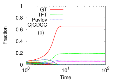
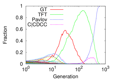
Although the RD description is more crude than the actual SPDG with local interactions, we find that the numerical integration of RD is surprisingly similar to what SPDG yields with the random initial distribution of strategies. In Fig. 3(b), it is displayed that the four nice strategies of GT, TFT, Pavlov, and $C|CDCC$ survive just like the previous observation made for SPDG. Furthermore, the order of relative fractions of the four is identical in both results. Note that these four strategies are indistinguishable at this stage, because the bits other than $a_{1}$ are not actually used any more. In order to slightly activate those bits and check how the surviving strategies behave in the presence of erroneous decisions, we allow each player in SPDG to make mistakes at a given probability $e$. For example, $e=0.01$ means that an agent’s memory on a neighbor’s last move may be flipped from $C$ to $D$ or $D$ to $C$, once in 100 moves on average. Depending on the initial condition, various steady-state configurations are obtained. In many cases, however, we find that Pavlov eventually conquers the whole territory, defeating TFT Nowak1993 , under such a low error rate (Fig. 4).

It is important that the error-free RD equilibrium selects out the long run strategies which appear in SPDG Tanimoto . The dynamics among these strategies are driven by errors in much larger time scales than the fast extinctions. When $e\ll 1$, the difference in these two time scales makes it possible to separate the fast extinctions from the long run behaviors. We point out that this selection can be further simplified, considering that each strategy occupies only a small fraction at the early stages and that the strategy with the least payoff decreases most rapidly. That is, the least fit strategy will be shortly removed from the population in effect, and the remainder’s payoffs are rectified accordingly. Eliminating the least fit actually reaches the same cooperating equilibrium with the minimal number of computations, and it works similarly to the technique called the iterated elimination of dominated strategies Borg . This procedure will be denoted as RD filtering since it is based on a fundamental assumption of RD that the growth rate of a species is proportional to its payoff. After it simulates the initial short times until reaching an equilibrium, we come back to SPDG and consider the slow dynamics due to errors among survivors. Nevertheless, we stress that this procedure is only a rough approximation and one should be careful not to expect general coincidence between them. Based on the numerical support in $M_{1}$, we are suggesting that this procedure can be regarded as a criterion that a feasible strategy is supposed to pass, rather than as a precise equivalent of SPDG. One obvious drawback is that it precludes much of the possibility of cyclic behaviors allowed by the continuous RD cycle , as we give the least fit no chance to return back (via, e.g, mutations) once removed.

III Application to $M_{2}$

III.1 Approach to memory effects

Let us proceed to the study of the strategies in $M_{2}$ to examine the effects of memory capacity in evolution. In order to decide the move at time $t$, an agent needs to remember her own moves and the opponent’s moves at $t-1$ and $t-2$, respectively, corresponding to $2^{4}=16$ bits. Until the agent meets the opponent more than once, the past information is not yet available and thus the strategy should specify the moves for this case with two more bits for the initial two encounters. Accordingly, the number of strategies in $M_{2}$ is counted as $|M_{2}|=2^{16+2}=262~{}144$. Based on the previous results for $M_{1}$, we use the same method to filter out unsuccessful strategies in an early stage, and then play SPDG only for surviving strategies.

Table 3: Strategy table for $M_{2}$.

Statea	$\Omega$ ($C$/$D$)b	ECc	ETd	I-TFTe	State	$\Omega$ ($C$/$D$)	EC	ET	I-TFT
($CC$,$CC$)	100/0	$C$	$C$	$C$	($DC$,$CC$)	50/50	$D$	$D$	$C$
($CC$,$CD$)	42/58	$C$	$C$	$D$	($DC$,$CD$)	45/55	-	-	$D$
($CC$,$DC$)	52/48	$D$	$D$	$C$	($DC$,$DC$)	50/50	$C$	$D$	$C$
($CC$,$DD$)	6/94	-	-	$D$	($DC$,$DD$)	47/53	-	-	$C$
($CD$,$CC$)	54/46	$C$	$C$	$D$	($DD$,$CC$)	52/48	-	-	$C$
($CD$,$CD$)	48/52	$C$	$C$	- f	($DD$,$CD$)	47/53	-	-	$C$
($CD$,$DC$)	56/44	-	-	$C$	($DD$,$DC$)	50/50	-	-	$C$
($CD$,$DD$)	31/69	-	-	$D$	($DD$,$DD$)	53/47	-	-	$D$

• ^a A state $(X_{1}X_{2},Y_{1}Y_{2})$ means that $X_{1}$ and $X_{2}$ ($Y_{1}$ and $Y_{2}$) are player’s (the opponent’s) moves at two subsequent times, respectively.

• ^b Percentages of $C$ and $D$ in $\Omega$, the set of the remaining strategies after RD filtering.

• ^c Efficient cooperator’s moves at each given state.

• ^d Efficient trigger’s moves. Although similar to EC’s, this does not follow EC at $(DC,DC)$ but defects it.

• ^e I-TFT’s moves. The moves at the recurrent states are underlined.

• ^f If both of $C$ and $D$ are observed, the move is written as blank.

III.2 RD filtering

In the filtering procedure for $M_{2}$, we again calculate $U_{ij}$ in the same way as before and use the mean-field payoff function in Eq. (1), assuming the full mixing. This reflects the fact that the initial strategies are randomly distributed and the number of remaining strategies turns out to be large enough to neglect clustering effects even at the equilibrium. The iterated elimination stops when no more strategies can be removed.

Figure 5: (Color online) Filtering procedure on $M_{2}$. It takes about $1.4\times 10^{5}$ steps to reach a cooperating equilibrium. (a) The remaining fraction $N/N_{t}$, where $N$ is the number of survivors and $N_{t}=2^{18}=262~{}144$. Insets show the two great extinction events at the $1424$th and $124~{}910$th steps, respectively. (b) The maximum and minimum values of the payoffs, divided by $N$. The straight line represents $R=3$, the reward for mutual cooperation. Insets and arrows are for the great extinction events again.

Figure 6: (Color online) Graphical representations of surviving strategies in $M_{2}$. (a) The full transition graph for I-TFT. Only the black vertices are recurrent states, while others are transient (see also Fig. 1). The dashed arcs indicate the paths activated when an error occurs between I-TFT’s. Since two strategies acting as I-TFT are found, we describe the duality in the graphs by the dotted arcs connected to two $(CD,CD)$ (at the top-left and the bottom). (b) Parts of transition graphs characterizing EC and ET. While an EC-typed strategy tries to recover mutual cooperation $(CC,CC)$ from an erroneous state $(CC,CD)$ by the dashed lines, an ET-typed strategy repeatedly defects it by the dotted line.

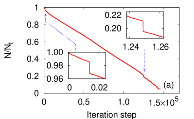
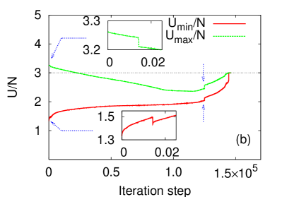
During $1.4\times 10^{5}$ steps to reach the goal, we record the number of remaining strategies $N$ and their expected payoffs $U$ ranged over $[U_{\rm min},U_{\rm max}]$. For comprehension, this range is divided by $N$ at each step in Fig. 5. Both of $U_{\rm min}/N$ and $U_{\rm max}/N$ eventually shrinks to a single point at $3.0$, indicating that all of the strategies obtain $R=3$ from mutual cooperation. From the concave shape of $U_{\rm max}/N$, we see two eras: Roughly before three-quarters of the whole period, $U_{\rm max}/N$ decreases by removing the least fit, as the top-ranked strategies exploit naive cooperators. After the prey is consumed out, however, they become the next victims. Removing defectors now enhances the degree of cooperation and $U_{\rm max}/N$ rises up as well. There are observed two great extinctions in that $2^{12}=4096$ strategies disappear simultaneously at the $1424$th and $124~{}910$th steps, respectively. These are symbolic of two eras, because AC is taken off at the first extinction and AD is at the second.

After completing the filtering procedure, we find an equilibrium, where $12~{}944$ surviving strategies constitute a set $\Omega$. The number is still large but only about 5% of $|M_{2}|$. There are two properties in this set: (i) All strategies in $\Omega$ are nice in the sense that they never defect first. (ii) After defected at the last two steps, about $94\%$ of the surviving strategies choose to retaliate. It is also remarkable that GT and TFT are included in $\Omega$ but Pavlov is dropped out.

Figure 7: (Color online) SPDG for $M_{2}$. (a) All of the $12~{}944$ strategies in $\Omega$ are initially distributed on $500\times 500$ lattices. They are classified as EC, ET, I-TFT and other miscellaneous ones, and the plotted values are averaged over $50$ realizations. (b) Three representative strategies belonging to EC, ET, and I-TFT, respectively, are distributed on a $32\times 32$ lattice. (c) Averaged results over 10 realizations on $500\times 500$ lattices, after removing two I-TFT strategies and their six similar variants (see text) from $\Omega$. There are given $p=0.02$ and $e=0.01$ in common.

III.3 Spatial Prisoner’s Dilemma Game for $M_{2}$

We next perform SPDG with $e>0$ for $\Omega$ on a two-dimensional $500\times 500$ lattice in the same manner as we did for $M_{1}$. Note that the lattice size is almost 20 times greater than the number of strategies, which turns out to be enough to find recognizably common patterns. After $2.4\times 10^{4}$ generations, most strategies in $\Omega$ also disappear and the number of survivors is usually less than 10 in each realization (Table 3).

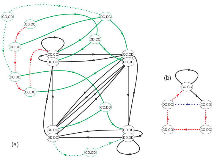
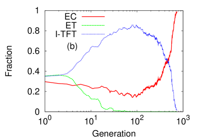
First, we observe two strategies with only eight recurrent states per each. They are named as intelligent-TFT (I-TFT) in common, because TFT is embedded as an attractor in their recurrent states and the transient states are activated only when an error occurs [Fig. 6(a)]. Again, the state $(X_{t}X_{t+1},Y_{t}Y_{t+1})$ represents that $X_{t}$ and $X_{t+1}$ ($Y_{t}$ and $Y_{t+1}$) are the player’s (the opponent’s) moves at two subsequent times ($X,Y=C$ or $D$), which is connected to $(X_{t+1}X_{t+2},Y_{t+1}Y_{t+2})$ by a directed arc. Without errors, they are ordinary TFT and never sucked repeatedly by any other strategies. With errors, on the other hand, they return back to mutual cooperation without the chain retribution between themselves, overcoming the weakness of the classical TFT. Furthermore, this error tolerance is secured from repeated abuse by being transient. We therefore conclude that the only way to defeat I-TFT is more efficient cooperation than I-TFT’s. As long as the error occurs rarely enough not to disturb its recovery path, I-TFT will clear the defecting strategies out and eventually make way for better cooperators.

Such efficient cooperators are characterized by the way of dealing with an error between themselves, depicted in Fig. 6(b) with the dashed lines. We denote those strategies with such an error recovery path as efficient cooperator (EC). An EC-typed strategy outperforms I-TFT because it costs less by one point in recovering an error. This one point may look small but has a significant meaning after thousands of generations. Yet an EC strategy can be invaded by even such a trivial strategy in $M_{1}$ as $\alpha|DDCC$ which simply alternate between $C$ and $D$, regardless of $\alpha$. That is, inserted among the strategies of $M_{1}$, an EC-typed strategy does not overwhelm $M_{1}$ and sometimes becomes exterminated. Meanwhile, I-TFT under the same condition works so successfully that it wins the whole area by defeating all of the $M_{1}$ strategies, including Pavlov, in every realization so long as $p$ is small enough.

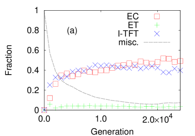
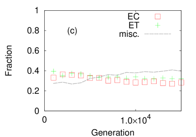
Last, some cooperating strategies are triggered to deceive EC by a single error: At the last step of EC’s error recovery phase, they defect again, instead of getting back to $(CC,CC)$ as desired, and complete the exploiting loop [see the dotted line in Fig. 6(b)]. Even if they are trigger strategies specialized to defeat EC, from which we simply call them efficient trigger (ET), I-TFT suppresses them and helps EC to rise [Figs. 7(a) and 7(b)].

Those two I-TFT strategies are distinguished by how they respond to the state $(CD,CD)$ (Table 3). Let us denote the I-TFT strategy responding with $C$ as I-TFT_C and that with $D$ as I-TFT_D. Comparing a population of I-TFT_C with that of I-TFT_D, the former is slightly better off, as the latter has a probability of $O(e^{2})$ that both players make errors at the same time, leading to $(CD,CD)\rightarrow(DD,DD)$ [Fig. 6(a)].

If we repeat this SPDG procedure after removing I-TFT from $\Omega$, some variants of I-TFT play the role of protecting EC. They have only one or two different bits from either of I-TFT strategies, but their recurrent states do not constitute TFT. Further removing such variants, we see that EC strategies are helplessly threatened by the parasitic ET [Fig. 7(c)]. Since ET strategies cannot do well with errors, the level of cooperation remains low. This comparison clearly shows the crucial role of I-TFT.

Let us recall Pavlov in comparison with EC: While GT and TFT ignored the presence of an error within the same species, not to be sucked by anyone, Pavlov invented a recovery path $(C,D)\rightarrow(D,D)\rightarrow(C,C)$ and could be the final winner in $M_{1}$. Nevertheless, it is at the very point that GT overruns Pavlov. It is therefore not surprising that Pavlov fails to enter $\Omega$, because so many strategies of $M_{2}$ are willing to exploit its shortsighted tolerance. Even though EC devises a more sophisticated recovery path than Pavlov’s, it is still far from safe. The point is that all of their states are recurrent: Even if they use every given memory capacity to determine the next move, once the patterns are recognized, the opponent can get back to the defecting state as many times as it wants. However, EC strategies are successful in the long run, because they try to cooperate better at some expense of security risk. The success of EC crucially depends on the existence of such balancing strategies as I-TFT, and is thus path-dependent.

IV Summary

In summary, we presented a thorough examination on strategies under restrictions of the time horizon in the iterated PD game. As the time horizon is enlarged, a variety of trajectories to equilibrium become possible, but there are still common dynamical patterns. That is, the system reaches efficient cooperation through intermediate prevalence of TFT-like strategies, which solve the dilemma between security and tolerance by using transient states. As I-TFT spends most time as the classical TFT which refers only to the opponent’s last move, it becomes even more likely to win if memory is costly Sethi . This gives a clue for understanding how the memory could be effectively saved in social interactions and differentiated into other functions.

The detailed features of our observation in this paper may be partially owing to our specific choice of elementary payoff values. However, we believe that the successful strategies such as I-TFT and dynamical patterns between them have good reasons to be remarkable in a more general context of the evolutionary PD game.