Tensor-entanglement renormalization group approach to topological phases
Abstract
The tensor-entanglement renormalization group approach is applied to Hamiltonians that realize a class of topologically ordered states – string-net condensed states. We analyze phase transitions between phases with and without string-net condensation. These phase transitions change topological order without changing any symmetries. This demonstrates that the tensor-entanglement renormalization group approach can be used to study the phase diagram of a quantum system with topologically ordered phases.
Introduction: A mean field approach could potentially be very useful for understanding and analyzing topological phasesWen (1995) and topological phase transitions.Wen and Wu (1993); Chen et al. (1993); Senthil et al. (1999); Read and Green (2000); Wen (2000, 2002); Levin and Wen (2006) The main challenges in developing such an approach are (a) finding a class of mean field states that can describe topological phases and (b) finding a simple way to calculate the physical properties, such as average energy, of these states. The first problem can be solved with a general class of trial wave functions known as “tensor product states” (or alternatively “projected entangled pair states”). Verstraete et al. (2006); Aguado and Vidal (2008) Indeed, one can show that tensor product states (TPS) can describe all the string-net condensed states constructed in Levin and Wen (2005), and hence all non-chiral topological phases. Gu et al. The second problem can be solved with the tensor-entanglement renormalization group (TERG) methodGu et al. (2008) which allows one to calculate correlation functions (including average energy) of a TPS very efficiently. More specifically, the relative error in a TERG calculation scales with the computation time like for 2D gapped systems. Gu et al. (2008) (For comparison, the error in a variational Monte Carlo calculation scales like , if there is no sign problem).
In this paper, we apply the TERG approach to a few models with string-net condensation. We calculate the phase diagram of these systems and study phase transitions from string-net condensed states to states without string-net condensation. These transitions are examples of continuous phase transitions between phases with different topological orders but the same symmetry.Wen and Wu (1993); Chen et al. (1993); Senthil et al. (1999); Read and Green (2000); Wen (2000, 2002) As such, they are beyond the Landau symmetry breaking paradigm. Thus the TERG approach is capable of describing phases and phase transitions that cannot be described by Landau’s symmetry breaking theory.
gauge model: The first system that we study is a spin-1/2 system where the spins live on links of a square lattice. The Hamiltonian is given by
| (1) |
Here is the product of the four around a square and sums over all the squares. is the product of the four around a vertex and sums over all the vertices. sums over all links. We will assume that and study the quantum phases of the above system as we change and . We will assume and .
When , eqn. (1) is exactly soluble.Kitaev (2003) To understand the exact ground state in the string language,Wen (2004) we interpret the and states on a single link as the presence or absence of a string. The appropriate low energy Hilbert space in large limit is made of closed string states that satisfy at every vertex. The ground state is simply an equal weight superposition of all closed string states , which is called a string-net condensed state.
When , the ground state is the spin polarized state with no down spins and no closed strings. The above two states have the same symmetry. But due to the non-trivial topological order in the string-net condensed state, the two states belong to two different quantum phases. We would like to use the TERG approach to study the phase transition between the above two states with different topological orders.
We would like to mention that the low energy effective theory of eqn. (1) is gauge theory.Read and Sachdev (1991); Wen (1991); Kitaev (2003) The transition between the string-net condensed and non condensed phases is nothing but the transition between the deconfined and confined phases of gauge theory.
One way to study such a phase transition is to introduce a variational wave function
| (2) |
where is the number of links on the string . When , becomes the string condensed state . When , is the state with all spins in up direction which does not contain any strings. We see that describes the string tension. is the ground state of eqn. (1) when and is the ground state of eqn. (1) when .
Since and have the same symmetry, one might expect that as we change , would change into smoothly and the ground state energy of eqn. (1) would be a smooth function of , implying that there was no quantum phase transition. In fact, we will see below that the ground state energy of eqn. (1) is not a smooth function of indicating that there is quantum phase transition at a critical value .

In order to calculate the energy expectation values in these states (and also to pave the way for generalizations) it is convenient to write the trial wave function as a tensor product state:
| (3) |
where labels the up-spin state and the down-spin state on link-. To define the tensor-trace (tTr), one can introduce a graphical representation of the tensors (see Fig. 1a). Then tTr means summing over all indices on the connected links of tensor-network. The string-net condensed ground state that we discussed above is given by the following choice of tensors:
| (6) |
| (7) |
with internal indices like running over . The rank-3 tensor behaves like a projector which essentially set the internal index equal to the physical index so that represents a string and represents no string. The meaning of the tensor is also clear, it just enforces the closed string constraint, only allowing an even number of strings to meet at a vertex.

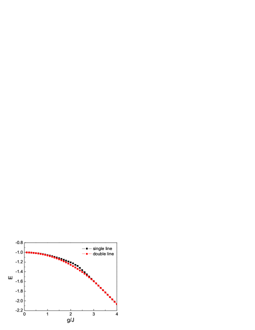
Once we have expressed the trial wave function as a TPS, we can use the TERG methodGu et al. (2008) to calculate the average energy in a very efficient way.111We can absorb the -tensor into the -tensor when we construct the double-tensor in the TERG calculation. The resulting average energy as a function of is plotted in Fig. 2. From the discontinuity in the slope, we see that there is a first order phase transition at between the two states with and without string-net condensation.
How good is this result? On a quantitative level, it is not very good: the phase transition is known to occur at .Blote and Deng (2002) However, this not surprising since we used the simplest possible variational wave function. We expect the estimate for to improve when we increase the number of variational parameters - for example, by considering more general tensors , .
A more serious problem is that the result is wrong on a qualitative level: the phase transition is known to be second order, not first order. This problem cannot be overcome by blindly generalizing the tensors , . Instead, we have to choose these tensors in a special way. To understand the basic issue, let us consider another set of variational tensors. In this scheme, the internal indices for the -tensors and -tensors still run from to , but each leg now has two internal indices:222The expression eqn. (8) is valid only on the sublattice A. The tensor has a slightly different form on the sublattice B. For details see eqn. (12) and Fig. 4.
| (8) | |||||
with and
| (9) |
In such constructions, our tensors have a double-line structure (see Fig.1b). Again, are projectors that relate the internal indices with physical indices. Here, on each leg of -tensor and -tensor, the double line with the same value is projected to the spin-up state and the double line with different values is projected to the spin-down state.
To maintain the degree rotational symmetry, we choose to have a form (assuming ):
| (10) |
We note that for such a choice of and , the trial wave function contain only closed string states.

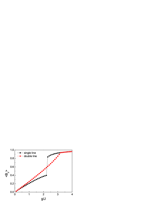
Using the TERG approach to minimize the average energy, we find the variational ground state energy which is plotted in Fig. 2. We find that there is a phase transition between the two phases with and without string-net condensation. But now the phase transition is a second order phase transition at (see Fig. 3). Note that this result is better than our previous result both quantitatively and qualitatively.
The quantitative improvement is perhaps not surprising since we are using more variational parameters. A more important issue is that the double-line mean field theory correctly predicts a second order phase transition, while the single line mean field theory did not. Why is this?
Note that there is a redundancy in the double-line tensors (like the gauge redundancy in gauge theory). As we exchange values of and for all the internal indices of the double-line tensors, we induce a transformation on those double-line tensors: . However, such a transformation does not change the physical wave function: . Thus and are two labels that label the same physical state.
The variational approach used here is similar to calculating an average in a local classical statistical system. The presence of a symmetry allows a classical system to have a symmetry breaking transition which is a second order phase transition. This is the reason why the double-line tensors are capable of producing a second order phase transition. In contrast, for the single-line tensors, the corresponding classical system does not have any symmetries, and as a result, it cannot describe a second order transition.
We would like to mention that there is a duality transformation that relate the 2D gauge theory to transverse field Ising model.Kogut (1979) Such a duality mapping allows us to relate the phase transition between the deconfined and confined phases of the gauge theory to the spin ordered and disordered transition in the transverse field Ising model. This is how we know that the transition between the string-net condensed and non condensed phases is a second order phase transition and that it occurs at critical coupling . In fact, the double-line tensors exactly realize the duality mapping between the 2D gauge theory and transverse field Ising model. From the structure of the double tensors in eqn. (9) and eqn. (Tensor-entanglement renormalization group approach to topological phases), we see that each square loops in Fig. 1b carries the same value of internal indices, which correspond to the value of a dual spin (located at the center of the square) in the dual Ising model. The string formed by the down-spins on the links correspond to a domain wall in the dual Ising model.

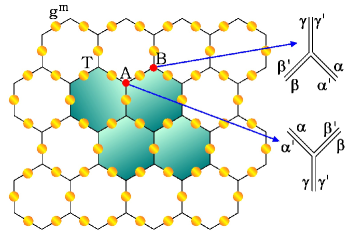
Double-semion model: Next we consider a more complicated model where spins are located on the links of a honeycomb lattice (see Fig. 4):
| (11) |
where i labels the links, I labels the vertices and p labels hexagons. Again we consider limit. When , the above model is exactly soluble and the exact ground state is given byLevin and Wen (2005) , where sums over all the closed string configurations and is number of closed loops in . The ends of string in such a state have the semion statistics. When , the model is also exactly soluble and the spins all point up (ie no strings) in the ground state.
To study the phase transition between the above two states, again we choose the double-line tensors to construct the trial wave function (see Fig. 4). The -tensors in the vertices are given schematically by
| (12) |
where each internal index represented by one of the double lines runs over . The tensor and is given by
| (13) |
The -tensors on the links are given by eqn. (9). The trial wave function is obtained by summing over all the internal indices on the connected links in the tensor network (see Fig. 4):
| (14) |
Again, the physical indices and the internal indices have a similar relation as in the double-line tensors. When , and , the tensor reproduces the right sign oscillations essentially by counting the number of left and right turns made by the string.

We used the TERG approach to find the variational ground states for different . Then we used the TERG approach to calculate for those variational ground states. The result is presented in Fig. 5. We see that there is a second order phase transition at , which should correspond to the transition between the string-net condensed and non condensed states. This agrees with the Monte Carlo result where a second order phase transition appears at .Blote and Deng (2002) (Note that in the infinite limit, the above model is equivalent to the usual gauge model on honeycomb lattice, which is dual to the transverse Ising model on triangle lattice.)
Conclusion: We have seen that the TERG approach is an effective way to study topological phases and topological phase transitions, but one needs to choose the variational tensors carefully. An important question is how to choose the tensors in more general situations. One hint is that all the string-net states constructed in LABEL:LWstrnet can be expressed naturally in terms of a generalization of the double-line tensor network, which involves triple line tensors.Gu et al. This triple-line tensor-network may correspond to the dual representation of the string-net states and may correspond to a suitable choice for the variational TERG approach. This may lead to a systematic variational approach for topological phases and topological phase transitions.
Acknowledgements: This research is supported by the Foundational Questions Institute (FQXi) and NSF Grant DMR-0706078.
References
- Wen (1995) X.-G. Wen, Advances in Physics 44, 405 (1995).
- Wen and Wu (1993) X.-G. Wen and Y.-S. Wu, Phys. Rev. Lett. 70, 1501 (1993).
- Chen et al. (1993) W. Chen, M. P. A. Fisher, and Y.-S. Wu, Phys. Rev. B 48, 13749 (1993).
- Senthil et al. (1999) T. Senthil, J. B. Marston, and M. P. A. Fisher, Phys. Rev. B 60, 4245 (1999).
- Read and Green (2000) N. Read and D. Green, Phys. Rev. B 61, 10267 (2000).
- Wen (2000) X.-G. Wen, Phys. Rev. Lett. 84, 3950 (2000).
- Wen (2002) X.-G. Wen, Phys. Rev. B 65, 165113 (2002).
- Levin and Wen (2006) M. Levin and X.-G. Wen, Phys. Rev. B 75, 075116 (2007).
- Aguado and Vidal (2008) M. Aguado and G. Vidal, Phys. Rev. Lett. 100, 070404 (2008).
- Verstraete et al. (2006) F. Verstraete, M. M. Wolf, D. Perez-Garcia, and J. I. Cirac, Phys. Rev. Lett. 96, 220601 (2006).
- Levin and Wen (2005) M. Levin and X.-G. Wen, Phys. Rev. B 71, 045110 (2005).
- (12) Z.-C. Gu, M. Levin, B. Swingle, and X.-G. Wen, to appear.
- Gu et al. (2008) Z.-C. Gu, M. Levin, and X.-G. Wen, arXiv:0806.3509 (2008).
- Kitaev (2003) A. Y. Kitaev, Ann. Phys. (N.Y.) 303, 2 (2003).
- Wen (2004) X.-G. Wen, Quantum Field Theory of Many-Body Systems – From the Origin of Sound to an Origin of Light and Electrons (Oxford Univ. Press, Oxford, 2004).
- Read and Sachdev (1991) N. Read and S. Sachdev, Phys. Rev. Lett. 66, 1773 (1991).
- Wen (1991) X.-G. Wen, Phys. Rev. B 44, 2664 (1991).
- Blote and Deng (2002) H. W. J. Blote and Y. Deng, Phys. Rev. E66, 066110 (2002).
- Kogut (1979) J. B. Kogut, Rev. Mod. Phys. 51, 659 (1979).