A many-flavor electron gas approach to electron-hole drops

Abstract

A many-flavor electron gas (MFEG) is analyzed, such as could be found in a multi-valley semiconductor or semimetal. Using the re-derived polarizability for the MFEG an exact expression for the total energy of a uniform MFEG in the many-flavor approximation is found; the interacting energy per particle is shown to be $-0.574447(E_{\text{h}}a_{0}^{3/4}m^{*3/4})n^{1/4}$ with $E_{\text{h}}$ being the Hartree energy, $a_{0}$ Bohr radius, and $m^{*}$ particle effective mass. The short characteristic length-scale of the MFEG motivates a local density approximation, allowing a gradient expansion in the energy density, and the expansion scheme is applied to electron-hole drops, finding a new form for the density profile and its surface scaling properties.

I Introduction

For some semiconductors, at low temperatures and high density, electrons and holes condense into electron-hole drops, which provide a good testing ground for understanding effects of electron-electron interactions Jeffries and Keldysh (1983). Some of the semiconductors (and also semimetals) that electron-hole drops form in Andryushin et al. (1976); Keldysh and Onishchenko (1976), such as Si, Ge, and diamond have conduction band minima near the Brillouin zone boundary, for example Si has six degenerate valleys, see Fig. 1, a Ge-Si alloy has ten degenerate valleys, and $\text{Pb}_{1-x-y}\text{Sn}_{x}\text{Mn}_{y}\text{Te}$ has twelve valleys in the $\Sigma$ band Story et al. (1990). When the material is strained, valley degeneracy reduces Brinkman and Rice (1973); Vashishta et al. (1974); Pokrovsky and Svistunova (1974); Vashishta and Das (1974); Kalia and Vashishta (1978), which can be experimentally probed Wolfe et al. (1978); Chou and Wong (1978); Wagner et al. (1981); Gourley and Wolfe (1981); Forchel et al. (1982); Culbertson and Furneaux (1982); Simon et al. (1989); Thonke et al. (2000); Jiang et al. (2005); Naka et al. (2007), meaning that valley degeneracy could be regarded as a control parameter. Because of this, as well as degeneracy being large in some semiconductors, valley degeneracy might be a good parameter with which to formulate a theory of electron-hole drops.

Previous theoretical analyses of electron-hole drops Sander et al. (1973); Rice (1974, 1977); Markiewicz et al. (1978); Markiewicz (1978); Kalia and Vashishta (1978); Reinecke et al. (1979) used an expansion of the energy density with parameters found from separate energy calculations Vashishta and Das (1974). An alternative approach is to assume that each valley contains a different type of fermion, denoted by an additional quantum number, which we shall call the flavor, the total number of flavors (valleys) is $\nu$. Further motivation to study flavors stems from the fact that in some previous studies of multiply degenerate systems the number of flavors has not been well defined, for example heavy fermions Zaránd et al. (2002); Kim (2005); Bolech and Iucci (2006), charged domain walls Eskes et al. (1998), a super-strong magnetic field Keldysh and Onishchenko (1976), and spin instabilities Giuliani and Quinn (1986); Marinescu et al. (2000). Cold atom systems in optical lattices Honerkamp and Hofstetter (2004a, b); Cherng et al. (2007) have a well defined number of flavors but weak interactions between particles. In electron-hole drops however the number of flavors is well defined and interactions are strong.

The ground state energy and pair correlation function of a free many-flavor electron gas (MFEG) were examined using a numerical self-consistent approach for the local field correction by Gold (1994), and superconductivity was studied by Cohen (1964). Following the method of Keldysh and Onishchenko (1976), Andryushin et al. (1976) studied the behavior of the free MFEG by summing over all orders of Green’s function contributions, they found an exact expression for the correlation energy of a MFEG (which dominates the interacting energy in the extreme many-flavor limit). This paper describes the derivation of a more versatile formalism, based on a path integral, which gives an exact expression for the total energy of the MFEG; the theory could apply with as few as six flavors where the exchange energy assumed small by Andryushin et al. (1976) would be significant.

As well as studying the uniform case, the previously unstudied density response of a MFEG not constrained to be uniform is investigated. The screening length-scales of the MFEG are shown to be short relative to the inverse Fermi momentum, suggesting that a local density approximation (LDA) might be a good approximation, motivating a gradient approximation. This gradient expansion is then applied to analyze the electron-hole drop density profile, and to simulate effects of strain the scaling of drop surface thickness and tension with number of flavors is examined.

Figure 1: The Si band structure in the $[100]$ direction generated with a LDA-DFT approximation by a plane-wave pseudopotential method Clark et al. (2005). The Fermi energy is as $E=0~{}\text{eV}$; below are valence bands with holes at H; above conduction bands, the bold parabolic curve signifies the first conduction band valley with electrons at E.

In a MFEG with $\nu$ flavors at low temperatures the relationship between the number density of electrons $n$ and Fermi momentum $p_{\text{F}}$ is

$$n=\frac{\nu p_{\text{F}}^{3}}{3\pi^{2}}.$$ (1)

When the electrons have multiple flavors, each Fermi surface encloses fewer states so $p_{\text{F}}\propto\nu^{-1/3}$. The local band curvature governs the electron effective mass, the band structure is often such that the holes relax into a single valence band minimum at the $\Gamma$ point (see Fig. 1); here holes are assumed to be heavy and spread out uniformly providing a jellium background.

The Thomas-Fermi approximation predicts a screening length $\kappa^{-1}=(4\pi e^{2}g)^{-1/2}$, where $g$ is the density of states (DOS) at the Fermi surface. The DOS is dependent on the number of flavors as $g\propto\nu\sqrt{E_{\text{F}}}\propto\nu^{2/3}$ and so $\kappa^{-1}\propto\nu^{-1/3}$. The ratio of the inverse Fermi momentum length-scale to the screening length varies with number of flavors as $p_{\text{F}}/\kappa\propto\nu^{-2/3}$. This paper takes the many flavor limit $\nu\gg 1$, in which the screening length is smaller than the inverse Fermi momentum, $\kappa^{-1}\ll p_{\text{F}}^{-1}$, the many-flavor limit therefore means that the wave vectors of the strongest electron-electron interactions obey $q\gg p_{\text{F}}$, this is the opposite limit to the RPA which assumes that $p_{\text{F}}\gg\kappa$. Physically this means the characteristic length-scales of the MFEG are short so a LDA can be used in Sec. III to develop a gradient expansion.

The conduction band energy spectrum is characterized by two spectra $E(\mathbf{q})$ and $\epsilon_{i}(\mathbf{p})$ as shown in Fig. 2. There are two energy functions: $E(\mathbf{q})$ gives the energy in the band structure at momentum $\mathbf{q}$; $\epsilon_{i}(\mathbf{p})=p^{2}/2m$ denotes the kinetic energy at momentum $\mathbf{p}$ with respect to the center of the $i\text{th}$ valley (the dispersions of all valleys are assumed to be the same and isotropic so that $\epsilon_{i}(\mathbf{p})=\epsilon(\mathbf{p})$. Andryushin et al. (1976) have outlined a method of calculating a scalar effective mass for anisotropic valleys).

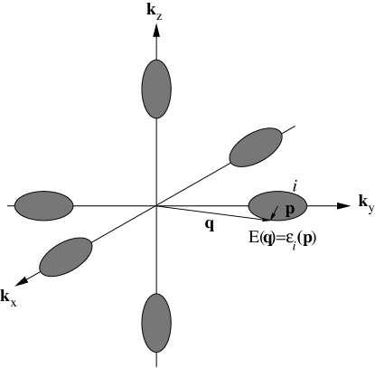
Figure 2: The dark grey ellipsoids show Fermi surfaces of electrons in the six degenerate conduction band valleys in Si. $E(\mathbf{q})$ is the energy with momentum $\mathbf{q}$ measured with respect to the $\Gamma$ point, $\epsilon_{i}(\mathbf{p})$ is energy with momentum $\mathbf{p}$ measured with respect to the center of the $i\text{th}$ valley.

Physical manifestations of the many-flavor limit include effects where the DOS at the Fermi surface (energy $E_{\text{F}}$) is important; from Eqn. (1) the DOS of a particular flavor $i$ shrinks as $g_{i}(E_{\text{F}})\propto p_{\text{F}}\propto\nu^{-1/3}$ whereas the DOS of all flavors grows since $g(E_{\text{F}})=\sum_{i=1}^{\nu}g_{i}(E_{\text{F}})=\nu g_{1}(E_{\text{F}})\propto\nu^{2/3}$. With increasing flavors, more electrons are within $\sim k_{\text{B}}T$ of the Fermi surface hence are able to be thermally excited, therefore the heat capacity of the MFEG, $C=12k_{\text{B}}^{2}T(\nu/3\pi^{2}n)^{2/3}/5$, increases with number of flavors. The Stoner criterion Kanamori (1963); Hubbard (1963) for band ferromagnetism states that for opposite spin electrons interacting with positive exchange energy $U$, ferromagnetism occurs when $g(E_{\text{F}})U\geq 1$. With increasing number of flavors the total DOS $g(E_{\text{F}})\propto\nu^{2/3}$ increases so that the Stoner criterion becomes more favorable. However, this analysis does not take into account the curvature of the DOS at the Fermi surface which can be an important factor in determining whether ferromagnetism occurs Wohlfarth and Rhodes (1962); Fabricius et al. (1993). The effect of the total DOS is also seen in the paramagnetic susceptibility, this is proportional to the total DOS at the Fermi surface so is expected to increase with number of flavors. Analogously one can compare a transition metal with narrow $d$-bands that leads to a large DOS at the Fermi surface with a simple metal that has broader free electron conduction bands and so a lower DOS at the Fermi surface. Similar to many flavor systems, transition metals are experimentally observed Ashcroft and Mermin (2001) to have a significantly higher specific heat capacity and greater magnetic susceptibility than typical simple metals. The simple scaling relationships with number of flavors for heat capacity and magnetization provide additional motivation to analyze a MFEG in more detail.

This paper uses the atomic system of units, that is $e^{2}=\hbar=m=1/(4\pi\epsilon_{0})=1$, but is modified so that $m$ denotes an appropriate effective mass for the electron-hole bands, which is the same for all valleys. This mass $m=m_{\text{e}}m^{*}$ can be expressed as a multiple of the electron mass $m_{\text{e}}$ and the dimensionless effective mass $m^{*}$. The units of length are then $a_{0}^{*}=a_{0}/m^{*}$ where $a_{0}$ is the Bohr radius, units of energy are those of an exciton, $E_{\text{h}}^{*}=E_{\text{h}}m^{*}$, where $E_{\text{h}}$ is the Hartree energy. These six quantities, defined to be unity, give the standard atomic units when $m^{*}=1$. For the important relationships that are derived in this paper particular to the MFEG, the full units are shown explicitly for clarity. Throughout this paper density is denoted by both $n$ (number density of particles) and $r_{\text{s}}$ (Wigner-Seitz radius).

In this paper, firstly a new formalism for the uniform system is derived. In Sec. I.1 the system polarizability is found, in Sec. II.1 the general quantum partition function is derived, and in Sec. II.2 the uniform MFEG total energy is calculated. Secondly, we examine the system with non-uniform density: in Sec. III a gradient expansion in the density for the total energy is found and is applied to electron-hole drops in Sec. IV, whose density profile and surface properties are calculated.

I.1 Polarizability

In this section the MFEG polarizability is derived. Though the result for the polarizability is the same as previous work Andryushin et al. (1976); Beni and Rice (1978), the derivation is presented here since an assumption made leads to an applicability constraint on the many-flavor theory (in Sec. II.3), and the MFEG polarizability is an important quantity that will feature prominently in two main results of this paper: the Sec. II derivation of the MFEG interacting energy and the derivation of the gradient expansion (see Sec. III).

The polarizability $\Pi_{0}^{\text{MF}}(\mathbf{q},\omega)$, where the superscript “MF” (many-flavor) denotes this is only for a MFEG, at wave vector $\mathbf{q}$ and Matsubara frequency $\omega$ is given by the standard Lindhard form

$$\Pi_{0}^{\text{MF}}(\mathbf{q},\omega)=\sum_{i,j=1}^{\nu}\frac{\delta_{i,j}}{4\pi^{3}}\int\frac{n_{{\text{F}}}\left(\epsilon_{i}\left(\mathbf{p}\right)\right)-n_{{\text{F}}}\left(\epsilon_{j}\left(\mathbf{p}+\mathbf{q}\right)\right)}{\text{i}\omega+\epsilon_{i}\left(\mathbf{p}\right)-\epsilon_{j}\left(\mathbf{p}+\mathbf{q}\right)}\text{d}\mathbf{p},$$ (2)

where $n_{\text{F}}(\epsilon_{i})=1/(\text{e}^{\beta(\epsilon_{i}-\mu)}+1)$ is the Fermi-Dirac distribution, $\beta=1/k_{\text{B}}T$, and $\mu$ is the chemical potential. In the standard expression for the polarizability the Fermi-Dirac distribution would contain the energy spectrum $E(\mathbf{p})$ but in the MFEG each electron is in a particular valley so the polarizability should be re-expressed in terms of the energy dispersion of each valley $\epsilon_{i}(\mathbf{p})$ (see Fig. 2) and the contributions must be summed over the valleys $i$ and $j$. Eqn. (II.2) shows that a large Coulomb potential energy penalty $V(\mathbf{q})\propto 1/q^{2}$ inhibits exchange between different valleys so that the Kronecker delta $\delta_{i,j}$ removes cross-flavor terms, and as all of the conduction valleys have the same dispersion a factor of $\nu$ will replace the remaining summation over valleys. Supposing each conduction valley has a locally quadratic isotropic dispersion relationship (with effective mass $m$), symmetrizing results in

$$\Pi_{0}^{\text{MF}}=\frac{\nu}{4\pi^{3}}\int\frac{n_{\text{F}}\left(\frac{1}{2}\left|\frac{1}{2}\mathbf{q}-\mathbf{p}\right|^{2}\right)-n_{\text{F}}\left(\frac{1}{2}\left|\frac{1}{2}\mathbf{q}+\mathbf{p}\right|^{2}\right)}{\text{i}\omega-\mathbf{p}\cdot\mathbf{q}}\text{d}\mathbf{p}.$$ (3)

In Sec. II.2 it is shown that the typical momentum exchange $q\sim(\hbar a_{0}^{-1/4})n^{1/4}$ is large relative to the Fermi momentum, therefore the two volumes in momentum space of integration variable $\mathbf{p}$, defined by the two Fermi-Dirac distributions are far apart relative to their radii $q/2\gg p_{\text{F}}$, and the temperature is sufficiently low so that the high energy tails of the two distributions have negligible overlap. Within these approximations the simple form for the polarizability is

$$\Pi_{0}^{\text{MF}}(\mathbf{q},\omega)=-\frac{n}{(\omega/q)^{2}+q^{2}/4},$$ (4)

this expression agrees with the many-flavor polarizability found by Andryushin et al. (1976) and Beni and Rice (1978).

The standard Lindhard form for the polarizability, when taken in the same $q\gg p_{\text{F}}$ limit as imposed by the many-flavor system agrees with Eqn. (4). In the static limit where frequencies are small compared to the momentum transfer $q^{2}\gg(\hbar^{3}/a_{0}^{*2}E_{\text{h}}^{*})\omega$, the polarizability varies as $q^{-2}$. In this limit, one Green’s function is restricted by the sum over Matsubara frequencies to lie inside the Fermi surface whilst the other gives the polarizability dependence of $1/\epsilon(\mathbf{q})\sim q^{-2}$ due to the excited electron’s kinetic energy.

The derivation of the polarizability accounted only for intra-valley scattering, which means that in the MFEG the same terms contribute Andryushin et al. (1976) as in the RPA for the standard electron gas. Therefore, diagrammatically, in the polarizability all electron loops are empty, the polarizability contains only reducible diagrams, which is denoted by the polarizability subscript “0”.

II Analytic formulation

Having reviewed the derivation of the polarizability of the system it is now used to formulate two complementary components of the many-flavor theory. The first is the derivation of the energy of a uniform system; we begin by calculating the general quantum partition function in Sec. II.1 and continue for the homogeneous case in Sec. II.2. The validity of the many-flavor approach for a uniform MFEG is investigated in Sec. II.3. The second part of the formalism is a gradient expansion of the energy density, looked at in Sec. III. Finally, the uniform and gradient expansion parts of the formalism will be brought together to study the model system of electron-hole drops in Sec. IV.

II.1 Partition function

To derive an expression for the total energy of the system a functional path integral method is followed, which is a flexible approach that should be extendable to investigate further possibilities such as modulated states and inter-valley scattering. Fermion field variables $\psi$ are used to describe the electrons irrespective of flavor in the dispersion $E(\mathbf{\hat{p}})$. Overall the system is electrically neutral, so in momentum representation the $\mathbf{q}=\mathbf{0}$ element is ignored. The repulsive charge-charge interaction acting between electrons is $V(\mathbf{r})=e^{2}/r$, we explicitly include the dependence on electron charge $e$ (even though it is defined to be unity) so that the charge can be set equal to zero to recover the non-interacting theory. For generality we consider stationary charges $Q(\mathbf{r})$ embedded in the MFEG which have a corresponding static potential $U(\mathbf{r})$. The quantum partition function for the MFEG written as a Feynman path integral is then

$$\mathcal{Z} = \iint\exp\left(\iint\bar{\psi}(\mathbf{r},\tau)\left(-\text{i}\hat{\omega}+E\left(\mathbf{\hat{p}}\right)-\mu\right)\psi(\mathbf{r},\tau)\text{d}\mathbf{r}\text{d}\tau\right)$$ (5)

$$\times \exp\left(\frac{1}{2}\iiint\left(\bar{\psi}(\mathbf{r^{\prime}},\tau)\psi(\mathbf{r^{\prime}},\tau)-Q(\mathbf{r^{\prime}})\right)V(\mathbf{r}-\mathbf{r^{\prime}})\left(\bar{\psi}(\mathbf{r},\tau)\psi(\mathbf{r},\tau)-Q(\mathbf{r})\right)\text{d}\mathbf{r}^{\prime}\text{d}\mathbf{r}\text{d}\tau\right)\mathcal{D}\bar{\psi}\mathcal{D}\psi.$$

This expression for the quantum partition function differs from that used for an electron gas (which has just a single flavor) only by the operator $E(\mathbf{\hat{p}})$ which gives the appropriate energy dispersion. To recover the standard electron gas result, which has a free particle dispersion relationship centered at the $\Gamma$ point, one should set $E(\mathbf{p})=p^{2}/2m_{\text{e}}$. For the MFEG, as outlined in Fig. 2, $E(\mathbf{p})$ represents the dispersion relationship of the whole conduction band, but no approximation concerning the flavors has yet been made, so the formalism applies for any number of flavors with a suitable energy dispersion relationship.

To make the action quadratic in the fermion variable $\psi$, the Hubbard-Stratonovich transformation Kleinert (1978) introduces an auxiliary boson field $\phi(\mathbf{r},\tau)$

$$\mathcal{Z} = \int\exp\Biggl{(}-\frac{\beta\Omega}{2}\sum_{\mathbf{q}\neq\mathbf{0},\omega}\phi(\mathbf{q},\omega)(q^{2}/4\pi)\phi(-\mathbf{q},-\omega)+\overbrace{\frac{\pi e^{2}\beta n}{2}\sum_{\mathbf{q}\neq\mathbf{0}}\frac{4\pi}{q^{2}}}^{\displaystyle{\dagger}}\Biggr{)}$$ (6)

$$\times \iint\exp\left(\iint\bar{\psi}(\mathbf{r},\tau)\left(-\text{i}\hat{\omega}+E\left(\mathbf{\hat{p}}\right)+\hat{U}-\mu+\text{i}e\hat{\phi}\right)\psi(\mathbf{r},\tau)\text{d}\mathbf{r}\text{d}\tau\right)\mathcal{D}\bar{\psi}\mathcal{D}\psi\mathcal{D}\phi.$$

The direct decoupling channel Kleinert (1978) was chosen as the relevant contributions come from a RPA-type contraction of operators.

The term labeled with a $(\dagger)$ exclusive of both fermion variables $\psi$ and the auxiliary field $\phi$, physically removes the electron self-interaction included when expressing the auxiliary field in a Fourier representation. Integrating over the fermion variables $\psi$ and using ${\ln}({\text{det}}\hat{A})={\operatorname{tr}}({\ln}\hat{A})$ gives $\mathcal{Z}=\int\text{e}^{-S[\phi]}\mathcal{D}\phi$, where the action $S[\phi]$ is

$$S[\phi] = \frac{\beta\Omega}{2\pi}\sum_{\mathbf{q}\neq\mathbf{0},\omega}\phi(\mathbf{q},\omega)(q^{2}/4\pi)\phi(-\mathbf{q},-\omega)$$ (7)

$$- 2\pi e^{2}\beta n\sum_{\mathbf{q}\neq\mathbf{0}}\frac{1}{q^{2}}$$

$$- {\operatorname{tr}}\bigl{(}{\ln}\bigl{(}\underbrace{-\text{i}\hat{\omega}+E\left({\mathbf{\hat{p}}}\right)+\text{i}e\hat{\phi}+\hat{U}-\mu}_{\displaystyle{\hat{G}_{\phi}^{-1}}}\bigr{)}\bigr{)}.$$

Due to its similarity to an inverse Green function, $\hat{G}_{\phi}^{-1}$ is used to denote the argument of the logarithm, the subscripts “$\phi$” or “$0$” denote whether the inverse Green’s function includes the auxiliary field or is free.

Finally, we note for use later that the ground state total energy per particle $E_{\text{G}}=E_{\text{int}}+E_{0}$ can be split into two components. The interacting energy is $E_{\text{int}}$ (found in Sec. II.2) and the non-interacting energy is

$$E_{0}=\frac{3}{10}\left(3\pi^{2}\frac{n}{\nu}\right)^{2/3},$$ (8)

which is the energy with interaction between charges switched off $(e=0)$. It falls with increasing number of electron flavors due to the shrinking Fermi surface.

II.2 Homogeneous Coulomb gas

So far, up to Eqn. (7), the formalism is exact, however to perform the functional integral over bosonic variable $\phi$ an approximation must be made. To proceed one notes that with no external potential $U(\mathbf{r})=0$ the saddle-point auxiliary field of the action (Eqn. (7)) is $\phi=0$, fluctuations in the action are expanded about the saddle point solution in $\phi$ giving the expression

$$S[\phi] = \ln(\hat{G}_{0}^{-1})+\operatorname{tr}\Bigl{(}\hat{\phi}\hat{V}^{-1}\hat{\phi}-\frac{1}{2}\overbrace{\hat{\phi}\hat{G}_{0}\hat{\phi}\hat{G}_{0}}^{\displaystyle{\ddagger}}\Bigr{)}$$ (9)

$$- \frac{1}{4}\operatorname{tr}\left(\hat{\phi}\hat{G}_{0}\hat{\phi}\hat{G}_{0}\hat{\phi}\hat{G}_{0}\hat{\phi}\hat{G}_{0}\right)+\mathcal{O}(\phi^{6})$$

$$- \frac{e^{2}}{2}\beta n\sum_{\mathbf{q}\neq\mathbf{0}}\frac{4\pi}{q^{2}}.$$

Terms are now kept to quadratic order in $\phi$, this is equivalent to the RPA, analogous to the terms kept in the derivation of the many-flavor polarizability, see Sec. I.1. This approximation will place a constraint on the validity of the formalism that is further examined in Sec. II.3.

The product of two Green’s functions in the quadratic term in $\phi$, labeled $(\ddagger)$, is identified with the polarizability $\Pi_{0}$, this is still expressed in terms of the general energy spectrum $E(\mathbf{p})$ so is not yet necessarily many-flavor and does not carry the superscript “MF” used in Sec. I.1. Following a multi-dimensional Gaussian integral over the fluctuating field $\phi$ (to quadratic order) the quantum partition function is

$$\mathcal{Z}=\prod_{\mathbf{q},\omega}\left(q^{2}/4\pi-e^{2}\Pi_{0}(\mathbf{q},\omega)\right)^{-\frac{1}{2}}\exp\left(\frac{\beta}{2}\sum_{\mathbf{q}\neq\mathbf{0}}\frac{4\pi e^{2}}{q^{2}}n\right).$$ (10)

In the low temperature limit we consider the free energy to get $E_{\text{G}}=-{\text{lim}}_{\beta\rightarrow\infty}({\ln}(\mathcal{Z})/\beta)=E_{\text{0}}+E_{\text{int}}$ to get the interacting energy per particle, normalized so that $E_{\text{int}}=0$ with no interactions $(e=0)$,

$$E_{\text{int}} = \frac{1}{2n}\Biggl{(}\iint{\ln}\left(1-\frac{4\pi e^{2}}{q^{2}}\Pi_{0}(\mathbf{q},\omega)\right)\frac{\text{d}\omega\text{d}\mathbf{q}}{(2\pi)^{4}}$$ (11)

$$- e^{2}n\sum_{\mathbf{q}\neq\mathbf{0}}\frac{4\pi}{q^{2}}\Biggr{)}.$$

This equation remains general and is not necessarily in the many-flavor limit, it is in agreement with previous expressions for the interacting energy Brinkman and Rice (1973) studied not in the many-flavor limit, but which use alternative forms for the polarizability. If the standard (single flavor) electron gas form for the polarizability, the Lindhard function, is used then it is possible to recover, in the high density limit, the Gell-Mann Brückner Gell-Mann and Brueckner (1957) expression for the total energy.

However, to proceed, one should now assume many-flavors and use the appropriate polarizability, Eqn. (4). The many-flavor polarizability summed over all Matsubara frequencies in the zero temperature limit $\beta\rightarrow\infty$ satisfies $\frac{1}{\beta}\sum_{\omega}\Pi_{0}^{\text{MF}}(\mathbf{q},\omega)=-n$. This is used to substitute for the electron density $n$ in the final term in Eqn. (11) to yield the many-flavor result

$$E_{\text{int}} = \frac{1}{2n}\iint\left(\ln\left(1-\frac{4\pi e^{2}}{q^{2}}\Pi_{0}^{\text{MF}}(\mathbf{q},\omega)\right)\right.$$ (12)

$$+ \left.\frac{4\pi e^{2}}{q^{2}}\Pi_{0}^{\text{MF}}(\mathbf{q},\omega)\right)\frac{\text{d}\omega\text{d}\mathbf{q}}{(2\pi)^{4}}.$$

To evaluate the interacting energy one first substitutes for the many-flavor polarization using Eqn. (4), makes the change of variables $\Omega=\omega/q^{2}$ and $Q=q/n^{1/4}$, and re-arranges to get

$$E_{\text{int}}=-n^{1/4}$$

$$\times\underbrace{\frac{1}{(2\pi)^{3}}\iint\frac{16\pi e^{2}}{1+4\Omega^{2}}-Q^{4}\ln\left(1+\frac{16\pi e^{2}/Q^{4}}{1+4\Omega^{2}}\right)\text{d}\Omega\text{d}Q}_{\displaystyle{A_{\text{3D}}}}.$$

The integral is independent of density and number of flavors, so is the numerical factor $A_{3\text{D}}=(E_{\text{h}}^{*}a_{0}^{*3/4})\Gamma(-5/4)\Gamma(3/4)/(2\pi^{5/4})\approx 0.574447(E_{\text{h}}^{*}a_{0}^{*3/4})$ that was evaluated analytically . The interacting energy is therefore

$$E_{\text{int}}=-A_{\text{3D}}n^{1/4},$$ (14)

which is independent of the number of flavors. In evaluating Eqn. (II.2) the main contribution to the integral over $Q=q/n^{1/4}$ is at a momentum $q\propto(\hbar a_{0}^{*-1/4})n^{1/4}$, so the interaction and screening length-scale in a MFEG is $\lambda\sim\hbar/q\propto a_{0}^{*1/4}n^{-1/4}\ll\hbar/p_{\text{F}}$, which is shorter than the Fermi momentum length-scale.

The interacting energy $E_{\text{int}}=E_{\text{ex}}+E_{\text{corr}}$ can be split into exchange energy $E_{\text{ex}}$ and correlation energy $E_{\text{corr}}$. The interacting energy is independent of number of flavors, the exchange energy, $E_{\text{ex}}=-(3/2)(3n/\pi\nu)^{1/3}$ Gold (1994), falls with number of flavors, therefore the correlation energy dominates over the exchange energy in the interacting energy in the many-flavor limit. In terms of the total energy, the correlation energy also dominates over the non-interacting energy, the kinetic energy that falls with number of flavors as $E_{0}\propto\nu^{-2/3}$. The increasing importance of the correlation energy can be understood further by considering the electron pair correlation function. With increasing number of flavors the length-scales between electrons of the same flavor increase as $\propto\nu^{1/3}r_{\text{s}}$ and thus exchange energy and kinetic energy reduce whereas the correlation energy depends only on the distance $r_{\text{s}}$ between electrons so is unaffected by the number of flavors present. Andryushin et al. (1976) and Keldysh and Onishchenko (1976) found the Eqn. (14) expression to be the correlation rather than interacting energy, neglecting the exchange energy which is small in the extreme many flavor limit. In Sec. II.3 the expression for the interacting energy is compared with self-consistent numerical calculations Gold (1994) on a MFEG with up to six flavors.

The interacting energy of a standard electron gas with a single flavor Gold (1994) is more negative than that of a MFEG, which in turn is more negative than that of a Bose condensate Gold (1992), this could be due to the reducing negativity of the exchange energy, important in the single flavor system, but zero in the Bose condensate. In these two extreme systems, the single flavor electron gas and the Bose condensate, there is no notion of valley degeneracy, and therefore the intermediate system, the MFEG, might be expected at most to have only a weak dependence on number of valleys. In fact, the interacting energy of the MFEG, over the range of density found in Sec. II.3, contains no dependence on the number of valleys. The absence of flavor dependence is also present in the universal behavior for the exchange-correlation energy in electron-hole liquids proposed by Vashishta and Kalia (1982).

The non-interacting energy term $E_{0}\propto(n/\nu)^{2/3}$ favors low electron density, the interacting term $E_{\text{int}}=-A_{\text{3D}}n^{1/4}$ favors high electron density, therefore the total energy per particle has a minimum as a function of density of $E_{\text{Gmin}}\propto-\nu^{2/5}$ at $n_{\text{min}}\propto\nu^{8/5}$. The presence of a minimum in energy with density of the MFEG is consistent with the results of Andryushin et al. (1976) and Brinkman and Rice (1973) who analyzed conduction electrons in a semiconductor. One consequence of this minimum is the possibility of a low density phase coexisting with excitons.

Before analyzing the non-uniform system in detail in Sec. III we can make qualitative arguments about its expected behavior within a potential well. According to Thomas-Fermi theory, an electron gas in a slowly varying attractive potential has a constant chemical potential. The electron gas is least dense at the edges of the potential and is densest at the center of the well. In a MFEG, due to the negative interacting energy $E_{\text{int}}=-A_{\text{3D}}n^{1/4}$ favoring high electron density, the density is expected to further reduce at the edges of the attractive potential and increase at the center of the well. In a repulsive potential the opposite should occur.

II.3 Density limits

In this section we will derive approximate expressions for the upper and lower density limits over which the many-flavor limit applies, these will be used to check the theory against numerical results Gold (1994) and to predict a lower bound on the number of flavors required for the theory to apply.

To find the upper density limit one notes that Eqn. (II.2) implies that an acceptable upper limit to the momentum integral would scale as $q=\alpha(\hbar a_{0}^{*-1/4})n^{1/4}$, the constant $\alpha\approx 4$ was determined numerically and was chosen to give the $q$ upper limit on the integral that recovered $95\,\%$ of the interacting energy. Additionally, the two regions of integration defined by the Fermi Dirac distributions in Eqn. (3) must not overlap, requiring that $q/2\geq p_{\text{F}}$. Combining these requires that for the many-flavor limit to apply the density must satisfy $na_{0}^{*3}\ll(\alpha^{12}\nu^{4})/(2^{12}3^{4}\pi^{8})$. Physically the breakdown at high density is due to the strongest interactions taking place on length-scales longer than the inverse length $p_{\text{F}}^{-1}$.

The low density limit is derived by considering the expansion of the action in the auxiliary boson field $\phi$, Eqn. (9). In order to evaluate the Gaussian functional integral over the bosonic variable $\phi$ it is necessary to neglect the quartic term in $\phi$, valid only when investigating the system with respect to its long-range behavior, that is $p_{\text{F}}\hbar a_{0}^{*}\gg 1$ Kleinert (1978), and therefore $na_{0}^{*3}\gg\nu/3\pi^{2}$. The breakdown at low density can be understood because the MFEG is effectively a boson gas, all electrons will be in the $\Gamma$ state ($\mathbf{k}=\mathbf{0}$) and there is no exchange energy.

The upper and lower critical density limits can be combined to conclude that the many-flavor limit result for interacting energy applies for densities that obey $0.03\nu\ll na_{0}^{*3}\ll 0.005\nu^{4}$; this density range increases as $\nu^{4}$ with number of flavors, the scaling relationship is the same as the applicable density range of the correlation energy found by Andryushin et al. (1976), though they did not provide estimates of numerical factors.

Using the above high and low density limits it is possible to estimate the minimum number of flavors required for the theory to apply. This is done by setting the lower and upper estimates for the allowable density to be equal, which gives $\nu\gtrapprox 2$, this estimate is approximate due to the possible inaccuracies in the upper and lower critical densities used in its derivation. As the upper and lower critical densities have been set equal, the many-flavor theory will apply here only over a very narrow range of densities, but this range widens with increasing number of flavors as $\nu^{4}$. An alternative limit can be found by comparing the interaction energy predicted by the theory over the expected density range of applicability with the results of Gold (1994). Their numerical self-consistent approach gives interaction energies accurate to approximately $3\,\%$ when compared with single-flavor electron gas quantum Monte Carlo (QMC) calculations Ceperley (1978); Ceperley and Alder (1980) and some initial many-flavor QMC calculations Conduit (2008). At two flavors the interacting energy predicted by the many-flavor theory is $\sim 10\,\%$ more positive than the self-consistent numerical results Gold (1994) indicating the many-flavor theory does not apply at two flavors. For six flavors over the predicted allowed density range the many-flavor theory is between $\sim 0\,\%$ and $\sim 4\,\%$ more positive than the numerical results, which indicates that the many-flavor theory can be applied within the predicted range of applicability ($0.5<r_{\text{s}}/a_{0}^{*}<1$). The theory should be applicable in common multi-valley compounds, such as silicon which has six conduction band valleys, and to those with more valleys Story et al. (1990). This result is corroborated by the results of initial QMC calculations Conduit (2008) on systems with between 6 and 24 flavors.

In the first half of this paper a new versatile formalism to describe a MFEG has been developed that could apply in systems containing approximately six or more degenerate conduction valleys. An exact expression for the total energy of the uniform MFEG was found and the applicable density range derived. The next step is to investigate the response of the MFEG to an external potential. A gradient approximation is developed in Sec. III and this is applied to electron-hole drops in Sec. IV.

III Gradient correction

In Sec. I it was shown that the typical length-scales of the MFEG are short $q\gg p_{\text{F}}$, motivating a local density approximation (LDA). This motivation is in addition to the usual reasons for the success of the LDA in density-functional theory (DFT) Payne et al. (1992) – that the LDA exchange-correlation hole need only provide a good approximation for the spherical average of the exchange-correlation hole and obey the sum rule Jones and Gunnarsson (1989). In this section the LDA is used with the polarizability derived in Sec. I.1 to develop a gradient correction to the energy density that allows the theory to be applied to a non-uniform MFEG.

The typical momentum transfer in the MFEG is $q\sim(\hbar a_{0}^{*-1/4})n^{1/4}$ hence the shortest length-scale over which the LDA may be made is approximately $(a_{0}^{*1/4}/\hbar)n^{-1/4}$ and the maximum permissible gradients in electron density are $|\nabla n|_{\text{max}}\sim qn\sim(\hbar a_{0}^{*-1/4}))n^{5/4}$. The gradient expansion will break down for short scale phenomena, for example a Mott insulator transition. To derive an energy density gradient expansion we follow Hohenberg and Kohn (1964) and Rice (1974) and consider an external charge distribution $n_{\text{ext}}(\mathbf{q})$ that couples to the induced charge distribution $n_{\text{ind}}(\mathbf{q})$ with Coulomb energy density

$$-\frac{1}{2}\sum_{\mathbf{q}}\frac{4\pi e^{2}}{q^{2}}n_{\text{ext}}(\mathbf{q})n_{\text{ind}}(\mathbf{q}).$$ (15)

One now substitutes for $n_{\text{ext}}(\mathbf{q})$ using the relative permittivity $1/\epsilon(\mathbf{q})=1+n_{\text{ind}}(\mathbf{q})/n_{\text{ext}}(\mathbf{q})=1/(1-4\pi\Pi_{0}^{\text{MF}}/q^{2})$ and the many-flavor polarizability Eqn. (4). The highest order term in $1/q^{2}$ gives the induced charge Coulomb energy, the term of order $q^{2}$ is associated with a gradient expansion, in real space this gives the expansion for the total energy per particle

$$E_{\text{G}}+\frac{(\nabla n)^{2}}{8n^{2}}+\mathcal{O}\left((\nabla n)^{4}\right),$$ (16)

here $E_{\text{G}}$ is ground state energy of the uniform system found in Sec. II.2. The form of the energy correction is similar to the von Weizsäcker term von Weizsäcker (1935), although here it is larger, having a coefficient of $1/8$ rather than $1/72$ as in the von Weizsäcker case. The difference can be qualitatively understood by considering the Fermi surfaces involved in the two cases for a given wave vector $q$, in the many-flavor case the Fermi surfaces involved in the integral of Eqn. (3) do not overlap as $q/2\gg p_{\text{F}}$ so there is a large volume in Fermi space available hence a large coefficient of $1/8$, whereas in the ordinary electron gas (single flavor) the same Fermi surfaces do overlap, as now $q/2\ll p_{\text{F}}$, reducing the volume available for integration so reducing the coefficient to $1/72$.

The gradient correction for the energy could be used in analytical approximations or as a DFT functional. This energy density expansion allows the MFEG to be applied to a variety of systems, its use for studying electron-hole drops is demonstrated in Sec. IV.

IV Electron-hole drops

In this section the MFEG is applied to a simple system to investigate the properties of, electron-hole drops. An electron-hole drop is a two-phase system: a spherical region of a MFEG surrounded by an exciton gas Beni and Rice (1978). The density profile, surface thickness and surface tension of drops are investigated; the scaling of surface thickness and tension with number of flavors is also found since this is can be experimentally probed through externally imposed strain reducing the valley degeneracy Pokrovsky and Svistunova (1974).

There have been four main theoretical methods used to analyze an electron-hole drop in silicon and germanium, semiconductors which have six and four flavors respectively. Rice (1977) fitted an analytic form to the energy density minimum and included the lowest order of a local gradient correction, from the equation for energy density an analytic form for the density profile was derived. A similar approach was used by Sander et al. (1973) and Rice (1974) to study the surface structure in more detail. The second approach Markiewicz et al. (1978); Markiewicz (1978), which was also applicable to situations with an external magnetic field and uniaxial strain, conserved momentum, particle number and pressure balance at the drop surface, the resulting equations were then solved numerically. A third approach followed by Kalia and Vashishta (1978) used a Padé approximant for the energy density Vashishta and Das (1974) derived specifically for silicon and germanium but did not include a gradient correction factor. The fourth approach of Reinecke et al. (1979) again used a Padé approximant for the energy density and also included a gradient correction factor. The latter two approaches assumed an exponential density profile for the drop. These four methods all use approximate forms for the energy density, an advantage of the many-flavor approach is that the exact form for the analytic energy density (within the many flavor assumption) can be used to solve for the drop density profile. Whilst analytic forms for the inner and outer density profile as well as a model for the entire profile can be derived, the general problem must be solved numerically. With an exact form for the density profile, electron-hole drop surface effects can be studied.

Local charge neutrality is assumed so that the density of electrons and holes are everywhere identically equal. A LDA with gradient correction is used so the drop energy density is written as the sum of the local non-interacting, local interacting and the lowest order term in a gradient expansion,

$$\varepsilon(\mathbf{r})=\frac{3}{10}\left(\frac{3\pi^{2}}{\nu}\right)^{2/3}n(\mathbf{r})^{5/3}-A_{3\text{D}}n(\mathbf{r})^{5/4}+\frac{(\nabla n(\mathbf{r}))^{2}}{8n(\mathbf{r})}.$$ (17)

The total energy of a drop is $\int\varepsilon(\mathbf{r})\text{d}\mathbf{r}$ and the total number of electrons in the drop is $\int n(\mathbf{r})\text{d}\mathbf{r}$. The total energy is minimized with respect to electron density $n(\mathbf{r})$ whilst keeping a constant number of electrons in the drop by applying the Euler-Lagrange equation with a Lagrange multiplier $\mu$, which represents the chemical potential. If the drop has spherical symmetry the density must satisfy

$$2rn\frac{\text{d}^{2}n}{\text{d}r^{2}}+4n\frac{\text{d}n}{\text{d}r}-r\left(\frac{\text{d}n}{\text{d}r}\right)^{2}$$

$$=16\left(\frac{3\pi^{2}}{\nu}\right)^{2/3}rn^{8/3}-40A_{3\text{D}}rn^{9/4}-32\mu rn^{2}.$$ (18)

The boundary conditions are specified at the center of the drop, where the density takes the equilibrium homogeneous MFEG value and the density is smooth, namely $n(0)=\bar{n}$ and $n^{\prime}(0)=0$. The differential equation Eqn. (IV) cannot be solved analytically for $n(\mathbf{r})$, but a solution, $n(\mathbf{r})=\bar{n}$, exists for $\mu=0$ which corresponds to the homogeneous MFEG, that is a drop containing an infinite number of electrons. Before solving the differential equation numerically, two approximate schemes are developed, one that applies near the drop center and the other near the drop edge, and their predictions are compared with existing density profile forms.

Near the center of the drop a perturbation solution about the equilibrium density, $n(\mathbf{r})=\bar{n}+\Delta n(\mathbf{r})$ where $\Delta n(\mathbf{r})\ll\bar{n}$, is considered. The solution to Eqn. (IV) for the density is then

$$n(r)=\bar{n}+\frac{8\mu\bar{n}}{Q^{2}}\left(1-\frac{\text{sinh}(Qr)}{Qr}\right).$$ (19)

This density profile is characterized by an exponential reduction of the density away from $\bar{n}$ at the center. The energy $Q^{2}$ is physically the rate of change of energy per unit volume with respect to changing particle density, with

$$Q^{2}=\frac{64}{3}\left(\frac{3\pi^{2}}{\nu}\right)^{2/3}\bar{n}^{2/3}-45A_{3\text{D}}\bar{n}^{1/4}-32\mu.$$ (20)

The second approximation scheme applies in the drop tail where electron density is low, $n(\mathbf{r})\ll\bar{n}$. The term containing the chemical potential is disregarded as it is arbitrarily small for the large drops under investigation, the non-interacting and interacting energy terms contain higher powers of density so are negligibly small. In this regime the solution to Eqn. (IV) is

$$n(r)=\begin{cases}n_{0}\left(\frac{1}{r}-\frac{1}{r_{0}}\right)^{2}&r<r_{0},\\ 0&r\geq r_{0}.\end{cases}$$ (21)

Here $n_{0}$ and $r_{0}$ are variational parameters which must be fitted to a numerical solution. This analytic form shows that the electron-hole drop has a definite outer radius $r_{0}$, which is approached parabolically, it is also noted that in the drop tail the solution obeys the differential equation

$$\frac{1}{r^{2}}\frac{\text{d}}{\text{d}r}\left(r^{2}\frac{\text{d}n^{1/2}}{\text{d}r}\right)=\nabla^{2}n^{1/2}=0.$$ (22)

If electron density is mapped onto a wave function $\psi$ through $n=|\psi|^{2}$ then the solution Eqn. (21) obeys Schrödinger’s equation at low energy, that is $\nabla^{2}\psi=0$. The implied Schrödinger equation is for a low density MFEG with negligible interaction between electrons due to their large separation, consistent with the original assumption of low density in the drop tail.

Previous studies of electron-hole drops Rice (1977); Kalia and Vashishta (1978); Reinecke et al. (1979) had a solution with the same exponential form both inside and outside of the drop, our inner functional form, an exponential, agrees with previous work Rice (1977); Kalia and Vashishta (1978); Reinecke et al. (1979), but our outer functional form, a quadratic-like polynomial, does not agree with the exponential decay seen in previous work. However, at the outside of the drop density is low and the arguments of Sec. II.3 show the many flavor theory, which requires that the density satisfies $n\gg 0.03\nu$, does not apply here. The other theories Rice (1977); Kalia and Vashishta (1978); Reinecke et al. (1979) also do not apply in the low density region so both the many-flavor and previous theories fail to agree only where they are not applicable.

Using just the solution for the density in the drop tail Eqn. (21), a reasonable analytical approximation for the density form of the whole drop is

$$n(r)=\left(\frac{1}{n_{0}(1/r-1/r_{0})}+\frac{1}{\bar{n}}\right)^{-1}.$$ (23)

This solution has the correct functional form at both the inside ($n(r)\rightarrow\bar{n}$) and outside of the drop and extrapolates smoothly in between. It can be fitted to the actual solution using parameters $n_{0}$ and $r_{0}$. However, the general differential equation is solved numerically giving the density profile shown in Fig. 3. The numerical solution is well approximated in the inner and outer regions by Eqn. (19) and Eqn. (21) respectively, and the model Eqn. (23) provides a good fit to the numerical solution, having just a slightly too shallow gradient around the median density but it agrees at both the center and outside of the well.

Figure 3: The density profile of a 12 flavor electron-hole drop with density parameter $r_{s}=1$. The numerical solution is shown by the dotted line, analytical approximations to the inside (outside) of the drop by the dashed (dot-dashed) lines, and a best fit model fitted to the numerical solution by the solid line.

To allow us to compare properties of electron-hole drops predicted using many-flavor theory with other work Kalia and Vashishta (1978); Reinecke et al. (1979), one can characterize the electron-hole drop properties through its surface thickness $D$ and tension $\gamma$. The surface thickness $D$ is the width over which the density falls from $90\,\%$ to $10\,\%$ of its homogeneous equilibrium value $\bar{n}$. The total surface energy is the difference between the energy per unit area of the MFEG in the drop and the energy of the same number of particles at equilibrium density in a homogeneous system. The surface tension $\gamma$ is the total surface energy divided by the characteristic drop surface area, here taken to be the area of the spherical surface at the median density, which corresponds to a characteristic drop radius $r_{\text{m}}$.

Figure 4: The surface tension $\gamma$ of the 12 flavor drop of radius $r_{\text{m}}$ is shown using the solid line and pluses based on the left-hand y-axis. The variation of the surface thickness $D$ is shown using the dashed line and crosses based on the right-hand axis, each point represents a separate simulation.

The results of numerical calculations in Fig. 4 show both the surface tension and surface thickness of the drop tend to constant values as the drop size increases. For large drops the boundary becomes approximately flat so the surface thickness becomes independent of drop radius, as does the surface tension since its major contribution comes from the drop boundary. We now examine the surface thickness and tension more carefully in turn.

To derive an approximate expression for the surface thickness we use the analytical approximation Eqn. (19) to the density profile of the inside of the drop, which gives the density reduction from the drop center

$$\Delta n(r)=-\frac{4\mu\bar{n}}{Q^{3/2}r}\text{e}^{Qr}.$$ (24)

From this, the surface thickness $D$ over which density falls from $90\,\%$ to $10\,\%$ is given in the large drop limit $r_{\text{m}}\gg D$ by

$$D\approx\frac{\ln 9}{Q}.$$ (25)

In the given example in Fig. 3 (12 flavors) this predicts that the surface thickness is $D\approx 0.8a_{0}^{*}$, which is of similar size to the result found by numerical solution of Eqn. (IV) of $\sim 1.1a_{0}^{*}$, but indicates that the approximation for surface thickness in Eqn. (25) is not able to produce accurate results. The values for surface thickness of drops found using the many-flavor theory can be compared with results from other approximations. For the six flavor gas in the large drop limit the many-flavor theory approximation Eqn. (25) predicts a thickness of $1.2a_{0}^{*}$, and exact numerical integration of the many-flavor theory Eqn. (IV) predicts thickness $1.6a_{0}^{*}$. The silicon six flavor result of Kalia and Vashishta (1978) has a surface thickness of $1.6a_{0}^{*}$, which is in good agreement with the many-flavor result.

Figure 5: The variation of surface tension (dashed line and crosses) and surface thickness (solid line and pluses) with number of flavors present, the straight line fits are used to give the exponents of the scaling parameters.

Having used many-flavor theory to predict the density profile and surface thickness of an electron-hole drop, it is interesting to examine their scaling relationships with number of flavors. This is because the scaling relationships can be experimentally probed Pokrovsky and Svistunova (1974) by comparing the surface thickness before and after putting the material under a strain which reduces the valley degeneracy, for example in silicon from six to two flavors. These scaling relations will also allow the many-flavor results to be further compared with previous theoretical work. In Sec. II.2 it was shown that the expected MFEG uniform density is $\bar{n}\propto\nu^{8/5}$, and from Eqn. (20) $Q^{2}\propto\nu^{2/5}$, which with Eqn. (25) predicts surface thickness to scale as $D\propto\nu^{-1/5}$. This scaling prediction for surface thickness can be compared with numerical results for the variation of surface thickness with number of flavors in Fig. 5, found by solving the differential equation Eqn. (IV). The coefficient for surface thickness $D\propto\nu^{\alpha}$ is $\alpha=-0.19995(7)$ in good agreement with the predicted value of $-1/5$. We can also qualitatively compare our scaling result with numerical results Kalia and Vashishta (1978); Reinecke et al. (1979) from studies of the electron-hole drop in silicon. These studies compared results for silicon found at the unstrained six flavor with the results at two flavors to attempt to model the effect of stress reducing valley degeneracy. Though two flavor calculations cannot be accurately given by the many-flavor theory, the qualitative variation of surface tension and surface thickness should be. The variation of surface thickness with number of flavors $D\propto\nu^{-1/5}$ is weak, for silicon from six to two flavors the many-flavor theory, assuming it is valid, predicts that the thickness increases by a factor of $1.2$. This compares reasonably with the numerical results of Ref. Kalia and Vashishta (1978), which predicts an increase in surface thickness by a factor of $\sim 1.1$.

The dominating contribution to surface energy is at the boundary of the drop so the surface tension in large drops is approximately the gradient term in the energy density, Eqn. (16) (the main contribution to the surface tension) multiplied by the surface thickness $D$

$$\gamma\approx\frac{(\nabla n)^{2}}{8\bar{n}}D\approx\frac{\bar{n}}{8D},$$ (26)

where we use the additional approximation $\nabla n\approx\bar{n}/D$. Finally, with the relationship found above, $D\propto\nu^{-1/5}$, and $\bar{n}\propto\nu^{8/5}$ found in Sec. II.2, this predicts surface tension varies with number of flavors as $\gamma\propto\nu^{9/5}$. The numerical results of Fig. 5, found by solving the differential equation Eqn. (IV) exactly, predict a coefficient for $\gamma\propto\nu^{\alpha}$ of $\alpha=1.8004(3)$ in good agreement with the analytical result, $9/5$. For silicon, reducing the number of flavors from six to two, the above result predicts that surface tension reduces by a factor of $7$. This qualitatively agrees with the variation seen by Refs. Kalia and Vashishta (1978); Reinecke et al. (1979) of a reduction by a factor of $3$, though comparison is difficult due to the presence of holes and there being too few flavors present for the many-flavor theory to be fully applicable.

V Conclusions

This paper describes a new formalism for calculating the behavior of a MFEG. In the many-flavor limit the Fermi momentum reduces as $p_{\text{F}}\propto\nu^{-1/3}$ so is small compared with the momenta associated with the strongest interactions. Intra-valley interactions are more significant than inter-valley.

The behavior of a homogeneous MFEG in the limit of many-flavors was derived. Specifically the exact interacting energy per particle is $E_{\text{int}}=-0.574447(E_{\text{h}}^{*}a_{0}^{*3/4}m^{*1/4})n^{1/4}$; making it energetically favorable for the MFEG to be dense. The formalism was found to apply with as few a six flavors over the density range $0.03\nu\ll na_{0}^{*3}\ll 0.005\nu^{4}$.

The MFEG has short characteristic length-scales which motivates a LDA. A gradient expansion of the energy density with the lowest order term $|\nabla n|^{2}/8n$ was derived, which was applied to electron-hole drops to study their density profile and surface properties. Surface thickness was found to scale as $D\propto\nu^{-1/5}$, surface tension as $\gamma\propto\nu^{9/5}$.

It would be useful to compare our analytical results with those from computer simulations to verify our findings for the uniform MFEG, its polarizability and the gradient expansion. This would allow the limits over which the many-flavor limit applies to be derived more accurately, and allow the formalism to be applied to more physical systems.