Universal Features in the Genome-level Evolution of Protein Domains

Protein domains are found on genomes with notable statistical distributions, which bear a high degree of similarity. Previous work has shown how these distributions can be accounted for by simple models, where the main ingredients are probabilities of duplication, innovation, and loss of domains. However, no one so far has addressed the issue that these distributions follow definite trends depending on protein-coding genome size only. We present a stochastic duplication/innovation model, falling in the class of so-called Chinese Restaurant Processes, able to explain this feature of the data. Using only two universal parameters, related to a minimal number of domains and to the relative weight of innovation to duplication, the model reproduces two important aspects: (a) the populations of domain classes (the sets, related to homology classes, containing realizations of the same domain in different proteins) follow common power-laws whose cutoff is dictated by genome size, and (b) the number of domain families is universal and markedly sublinear in genome size. An important ingredient of the model is that the innovation probability decreases with genome size. We propose the possibility to interpret this as a global constraint given by the cost of expanding an increasingly complex interactome. Finally, we introduce a variant of the model where the choice of a new domain relates to its occurrence in genomic data, and thus accounts for fold specificity. Both models have general quantitative agreement with data from hundreds of genomes, which indicates the coexistence of the well-known specificity of proteomes with robust self-organizing phenomena related to the basic evolutionary “moves” of duplication and innovation.

Introduction

The availability of many genome sequences gives us abundant information, which is, however, very difficult to decode. As a consequence, in order to advance our understanding of biological processes at the whole-cell scale, it becomes very important to develop higher-level descriptions of the contents of a genome. At the level of the proteome, an effective scale of description is provided by protein domains OT05 . Domains are the unit-shapes (or “folds”) forming proteins BT99 . They constitute independent thermodynamically stable structures. A domain determines a set of potential functions and interactions for the protein that carries it, for example DNA- or protein-binding capability or catalytic sites KWK02 ; OT05 . Therefore, domains underlie many of the known genetic interaction networks. For example, a transcription factor or an interacting pair of proteins need the proper binding domains MBT03 ; NBG+05 , whose binding sites define transcription networks and protein-protein interaction networks respectively.

Protein domains are related to sets of sequences of the protein-coding part of genomes. Multiple sequences give rise to the same shape, and the choice of a specific sequence in this set fine-tunes the function, activity and specificity of the inherent physico-chemical properties that characterize a shape. A domain then defines naturally a “domain class”, constituted by all its realizations in the genome, or all the proteins using that given shape for some function. Overall, domains can be seen as an “alphabet” of basic elements of the protein universe. Understanding the usage of domains across organisms is as important and challenging as decoding an unknown language. Much as the letters of linguistic alphabets, the domains observable today are few, probably of the order of $10^{5}$ KWK02 . This number is surprisingly lower than the number of possible protein sequences (which are in general a hundred orders of magnitude more numerous). In the course of evolution, domains are subject to the dynamics of genome growth (by duplication, mutation, horizontal transfer, gene genesis, etc.) and reshuffling (by recombination etc.), under the constraints of selective pressure KWK02 ; QLG01 . These drives for combinatorial rearrangement, together with the defining modular property of domains, lead to the construction of increasingly richer sets of proteins RBT+04 . In other words, domains are particularly flexible evolutionary building blocks.

In particular, the sequences of two duplicate domains that diverged recently will be very similar, so that one can also give a strictly evolutionary definition of protein domains KWK02 , as regions of a protein sequence that are highly conserved. The (interdependent) structural and evolutionary definitions of protein domains given above have been used to produce systematic hierarchical taxonomies of domains that combine information about shapes, functions and sequences MBH+95 ; OMJ+97 . Generally, one considers three layers, each of which is a subclassification of the previous one. The top layer of the hierarchy is occupied by “folds”, defined by purely structural means. It is then possible, though it seems quite rare, that a fold is polyphyletic, i.e. found from different paths in evolution. The intermediate “superfamily” class is also mainly defined by spatial shape, with the aid of sequence and functional annotations to guarantee monophyly. Finally, the “family” class is defined by sequence similarity.

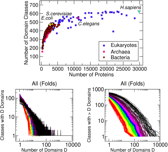
The large-scale data stemming from this classification effort enable to tackle the challenge of understanding the alphabet of protein domains RST+06 ; OT05 ; BBK+05 ; WBB06 . In particular, they have been used to evaluate the laws governing the distributions of domains and domain families HvN98 ; QLG01 ; KWR+02 ; Kuz02 ; AD05 . As noted by previous investigators, these laws are notable and have a high degree of universality. We reviewed these observations performing our own analysis of data on folds and superfamilies from the SUPERFAMILY database WMV+07 (Supplementary Note S2). Using the number of domains $n$ to measure the size of a genome, we have the following observations, that confirm (and in part extend) previous ones.

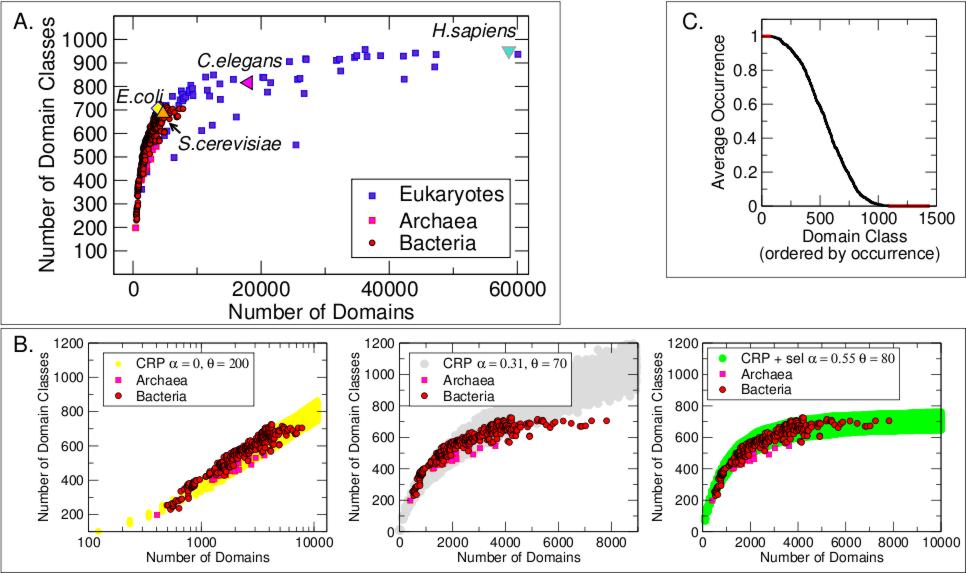
• The number of domain families (or distinct hits of the same domain) concentrates around a curve $F(n)$ that is markedly sublinear with size (figure 2A), perhaps saturating.

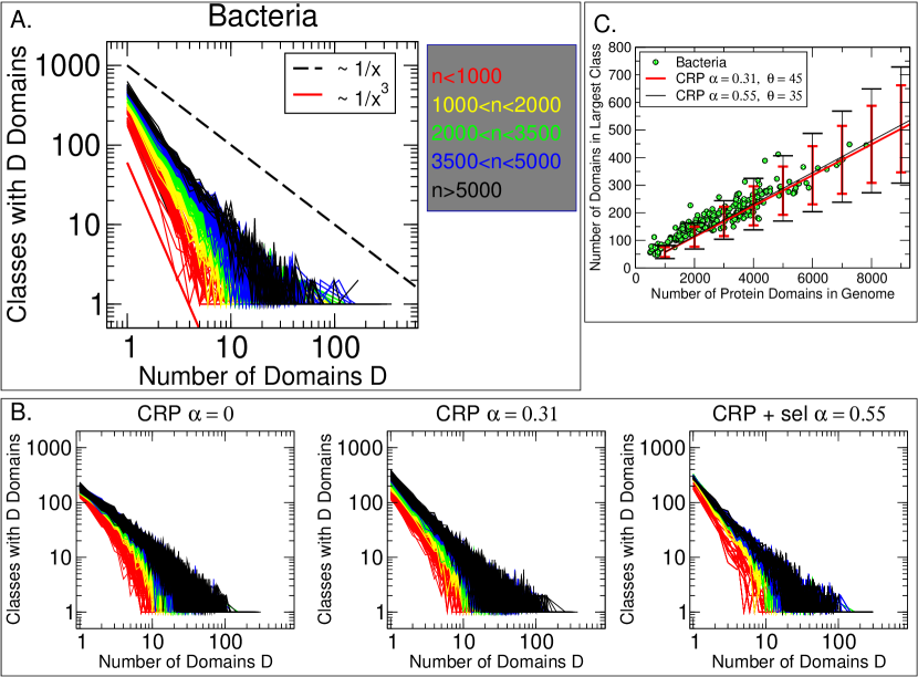
• The number $F(j,n)$ of domain classes having $j$ members (in a genome of size $n$) follows the power-law $\sim 1/j^{1+\alpha}$, where the fitted exponent $1+\alpha$ typically lies between 1 and 2 (figure 3).

• The fitted exponent of this power-law appears to decrease with genome size (figure 3A), and there is evidence for a cutoff that increases linearly with $n$ (figure 3C).

Recent modeling efforts focused mainly on observation (ii), or the fact the the domain class distributions are power laws. They explored two main directions. First, a “designability” hypothesis LTW98 , which claims that domain occurrence is due to accessibility of shapes in sequence space. While the debate is open, this alone seems to be an insufficient explanation, given for example the monophyly of most folds in the taxonomy KWK02 ; DS07 . A second, “genome growth” hypothesis ascribing the emergence of power-laws to a generic preferential-attachment principle due to gene duplication seems to be more successful. Growth models were formulated as nonstationary, duplication-innovation models QLG01 ; KLQ+06 ; DS05 , and as stationary birth-death-innovation models KWR+02 ; KWK03 ; KWB+04 ; KBK05 . They were successful in describing to a consistent quantitative extent the observed power laws. However, in both cases, each genome was fitted by the model with a specific set of kinetic coefficients, governing duplication, influx of new domain classes, or death of domains. Another approach used the same modeling principles in terms of a network view of homology relationships within the collective of all protein structures DSS02 ; Dok05

On the other hand, the common trend for the number of domain classes at given genome size and the common behavior of the observed power laws in different organisms having the same size (observations i-iii above), call for a unifying behavior in these distributions, which has not been addressed so far. Here, we first define and relate to the data a non-stationary duplication-innovation model in the spirit of Gerstein and coworkers QLG01 . Compared to this work, our main idea is that a newly added domain class is treated as a dependent random variable, conditioned by the preexisting coding genome structure in terms of domain classes and number. We will show that this model explains observations (i-iii) with a unique underlying stochastic process having only two universal parameters of simple biological interpretation, the most important of which is related to the relative weight of adding a domain belonging to a new family and duplicating an existing one. In order to reproduce the data, the innovation probability of the model has to decrease with proteome size, i.e. such as it is less likely to find new domains in genomes with increasingly larger number of domains. This feature is absent in previous models, and we suggest the possibility to interpret it as a consequence of the computational cost for adding a new domain class in a genome. This cost could be associated to a rewiring in the existing regulatory interaction networks, needed to accomodate an new domain class, correspondong to an extra set of functions. Finally, we show how the specificity of domain shapes, introduced in the model using empirical data on the usage of domain classes across genomes, can improve quantitative agreement of the model with data, and in particular predict the saturation of the number of domain classes $F(n)$ at large genome sizes.

Model and Results

Main Model

Ingredients.

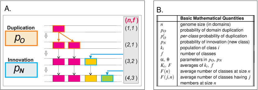
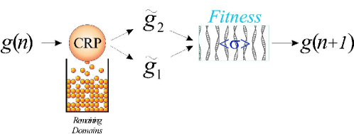
An illustration of the model and a table resuming the main parameters and observables are presented in figure 1. The basic ingredients of the model are $p_{O}$, the probability to duplicate an old domain (modeling gene duplication), and $p_{N}$, the probability to add a new domain class with one member (which describes domain innovation, for example by horizontal transfer). Iteratively, either a domain is duplicated with the former probability or a new domain class is added with the latter.

An important feature of the duplication move is the (null) hypothesis that duplication of a domain has uniform probability along the genome, and thus it is more probable to pick a domain of a larger class. This is a common feature with previous models QLG01 . This hypothesis creates a “preferential attachment” principle, stating the fact that duplication is more likely in a larger domain class, which, in this model as in previous ones, is responsible for the emergence of power-law distributions. In mathematical terms, if the duplication probability is split as the sum of per-class probabilities $p_{O}^{i}$, this hypothesis requires that $p_{0}^{i}\propto k_{i}$, where $k_{i}$ is the population of class $i$, i.e. the probability of finding a domain of a particular class and duplicating it is proportional to the number of members of that class.

It is important to notice that in this model, while $n$ can be used as an arbitrary measure of time, the weight ratio of innovation to duplication at a given $n$ is not arbitrary, and is set by the ratio $p_{N}/p_{O}$. In the model of Gerstein and coworkers, both probabilities, and hence their ratio, are constant. In other words the innovation move is considered to be statistically independent from the genome content. This choice has two problems. First, it cannot give the observed sublinear scaling of $F(n)$. Indeed, if the probability of adding a new domain is constant with $n$, so will be the rate of addition, implying that this quantity will increase on average linearly with genome size. It is fair to say that Gerstein and coworkers do not consider the fact that genomes cluster around a common curve (as shown by the data in figure 2) and think each of them as coming from a stochastic process with genome-specific parameters. Second, their choice of constant $p_{N}$ implies that for larger genomes the influx of new domain families is heavily dominant on the flux of duplicated domains. This again contradicts the data, where additions of new domain classes are rarer with increasing genome size.

Defining Equations and Chinese Restaurant Process.

On the contrary, motivated by the sublinear scaling of the number of domain classes (observation (i)), we consider that $p_{N}$ is conditioned by genome size. We observe (see ref. DS05 ) that constant $p_{N}$ makes sense thinking that new folds emerge from a mutation process with constant rate rather than from an external flux. This flux, coming from horizontal transfer, could be thought of as a rare event with Poisson statistics and characteristic time $\tau$, during which the influx of domains is $\Theta\tau$. In this case it is immediate to verify that $f(n)$ has mean value given by $\sum_{j=1}^{n}\frac{\Theta}{\Theta+n}$ thus growing as $\Theta\log n$. This scenario is complementary to the one of Gerstein and coworkers because old domain classes limits the universe that new classes can explore.

One can think of intermediate scenarios between the two. The simplest scheme, which turns out to be quite general, implies a dependence of $p_{N}$ by $n$ and $f$, where $n$ is the size (defined again as the total number of domains) and $f$ is the number of domain classes in the genome. Precisely, we consider the expressions

$$p_{O}^{i}=\frac{k_{i}-\alpha}{n+\theta}$$

, hence, since $p_{O}=\sum_{i}p_{O}^{i}$,

$$p_{O}=\frac{n-\alpha f}{n+\theta}\ \ ,$$

and

$$p_{N}=\frac{\theta+\alpha f}{n+\theta}\ \ ,$$

where $\theta\geq 0$ and $\alpha\in[0,1]$. Here $\theta$ is the parameter representing a characteristic number of domain classes needed for the preferential attachment principle to set in, and defines the behavior of $f(n)$ for small $n$ ( $n\rightarrow 0$). $\alpha$ is the most important parameter, which will set the scaling of the duplication/innovation ratio (table 1), Intuitively, for smaller $\alpha$ the process slows down the growth of $f$ at smaller values of $n$ ( necessarily $f<n$ ); and since $p_{N}$ is asymptotically proportional to the class density $f/n$, it is harder to add a new domain class in a larger, or more heavily populated genome. As we will see, this implies $p_{N}/p_{O}\rightarrow 0$ as $n\rightarrow\infty$, corresponding to an increasingly subdominant influx of new fold classes at larger sizes. We will show that this choice reproduces the sublinear behavior for the number of classes and the power-law distributions described in properties (i-iii).

This kind of model has previously been explored in a different context in the mathematical literature under the name of Pitman-Yor, or Chinese Restaurant Process (CRP) Pit02 ; PY97 ; Ald85 ; Kin75 . In the Chinese restaurant metaphor, domain realizations correspond to customers and tables are domain classes. A domain which is member of a given class is a customer sitting at the corresponding table. In a duplication event, a new customer is seated at a table with a preferential attachment (or packing) principle, and in an innovation event, a new table is added.

Theory and Simulation.

We investigated this process using analytical asymptotic equations and simulations. The natural random variables involved in the process are $f$, the number of tables or domain classes, $k_{i}$ the population of class $i$, and $n_{i}$, the size at birth of class $i$. Rigorous results for the probability distribution of the fold usage vector $\{k_{1},...,k_{f}\}$ confirm the results of our scaling argument. It is important to note that in this stochastic process, large $n$ limit values of quantities such as $k_{i}$ and $f$ do not converge to numbers, but rather to random variables Pit02 .

Despite of this property, it is possible to understand the scaling of the averages $K_{i}$ and $F$ (of $k_{i}$ and $f$ respectively) at large $n$, writing simple “mean-field” equations, for continuous $n$. From the definition of the model, we obtain $\partial_{n}K_{i}(n)=\frac{K_{i}-\alpha}{n+\theta}$, and $\partial_{n}F(n)=\frac{\alpha F(n)+\theta}{n+\theta}$. These equations have to be solved with initial conditions $K_{i}(n_{i})=1$, and $F(0)=1$. Hence, for $\alpha\neq 0$, one has $K_{i}(n)=(1-\alpha)\frac{n+\theta}{n_{i}+\theta}+\theta$, and

$$F(n)=\frac{1}{\alpha}\left[(\alpha+\theta)\left(\frac{n+\theta}{\theta}\right)^{\alpha}-\theta\right]\sim n^{\alpha}\ \ ,$$

while, for $\alpha=0$

$$F(n)=\theta\log(n+\theta)\sim\log(n)\ \ .$$

These results imply that the expected asymptotic scaling of $F(n)$ is sublinear, in agreement with observation (i).

The mean-field solution can be used to compute the asymptotics of $P(j,n)=F(j,n)/F(n)$ BA99 . This works as follows. From the solution, $j>K_{i}(n)$ implies $n_{i}>n^{*}$, with $n^{*}=\frac{(1-\alpha)n-\theta(j-1)}{j-\alpha}$, so that the cumulative distribution can be estimated by the ratio of the (average) number of domain classes born before size $n^{*}$ and the number of classes born before size $n$, $P(K_{i}(n)>j)=F(n^{*})/F(n)$. $P(j,n)$ can be obtained by derivation of this function. For $n,j\rightarrow\infty$, and $j/n$ small, we find

$$P(j,n)\sim j^{-(1+\alpha)}$$

for $\alpha\neq 0$, and

$$P(j,n)\sim\frac{\theta}{j}$$

for $\alpha=0$. The above formulas indicate that the average asymptotic behavior of the distribution of domain class populations is a power law with exponent between $1$ and $2$, in agreeement with observation (ii).

The trend of the model of Gerstein and coworkers can be found for constant $p_{N},\ p_{O}$ and gives a linearly increasing $F(n)$ and a power-law distribution with exponent larger than $2$ for the domain classes. A comparative scheme of the asymptotic results is presented in table 1. We also verified that these results are stable for introduction of domain loss and global duplications in the model (see Supplementary Note S4). Incidentally, we note that also the “classic” Barabasi-Albert preferential attachment scheme BA99 can be reproduced by a modified model where at each step a new domain family (or new network node) with on average $m$ members (edges of the node) is introduced, and at the same time $m$ domains are duplicated (the edges connecting old nodes to the new node).

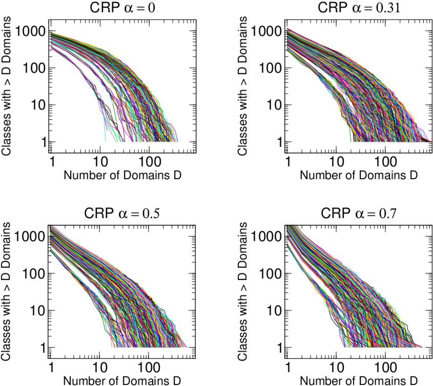
Going beyond scaling, the probability distributions generated by a CRP contain large finite-size effects that are relevant for the experimental genome sizes. In order to evaluate the behavior and estimate parameter values keeping into account stochasticity and the small system sizes, we performed direct numerical simulations of different realizations of the stochastic process (figures 2B and 3B and C). The simulations allow to measure $f(n)$, and $F(j,n)$ for finite sizes, and in particular for values of $n$ that are comparable to those of observed genomes. At the scales that are relevant for empirical data, finite size corrections are substantial. Indeed, the asymptotic behavior is typically reached for sizes of the order of $n\sim 10^{6}$, where the predictions of the mean-field theory are confirmed.

Comparing the histogram of domain occurrence of model and data, it becomes evident that the intrinsic cutoff set by $n$ at the causes the observed drift in the fitted exponent described in observation (iii), and shown in figure 3A and B. In other words, the observed common behavior of the slopes followed by the distribution of domain class population for genomes of similar sizes can be ascribed to finite-size effects of a common underlying stochastic process. We measured the cutoff of the distributions as the population of the largest domain class, and verified that both model and data follow a linear scaling (figure 3C). This can be expected from the above asymptotic equations, since $K_{i}(n)\sim n$.

The above results show that the CRP model can reproduce the observed qualitative trends for the domain classes and their distributions for all genomes, with one common set of parameters, for which all random realizations of the model lead to a similar behavior. One further question is how quantitatively close the comparison can be. To answer this question, we compared data for the bacterial data sets and models with different parameters. Although the agreement is reasonably good, this comparison makes it difficult to decide between a model with $\alpha=0$ and a model with finite (and definite) $\alpha$: while the slope of $F(n)$ is more compatible with a model having $\alpha=0$, the slopes of the internal power-law distribution of domain families $P(j,n)$ and their cutoff as a function of $n$ is in closer agreement to a CRP with $\alpha$ between 0.5 and 0.7 (figure 2B and Supplementary Note S1 and S2).

Domain Family Identity and Model with Domain Specificity

We have seen that the good agreement between model and data from hundreds of genomes is universal and realization-independent . On the other hand, although one can clearly obtain from the basic model all the qualitative phenomenology, the quantitative agreement is not completely satisfactory, as both qualitative behaviors observed in the model for $\alpha=0$ and $\alpha>0$ seem to agree better with only one between the two main observables: domain distributions and observed domain family number (figure 2 and 3).

We will now show how a simple variant of the model that includes a constraint based on empirically measured usage of individual domain classes can bypass the problem, without upsetting the underlying ideas presented above. Indeed, there exist also specific effects, due to the precise functional significance and interdependence of domain classes. These give rise to correlations and trends that are clearly visible in the data, which we have analyzed more in detail in a parallel study HSB+ . Here, we will consider simply the empirical probabilities of usage of domain families for 327 bacterial genomes in the SUPERFAMILY database WMV+07 (figure 2C). These observables are largely uneven and functional annotations clearly show the existence of ubiquitous domain classes, which correspond to “core” or vital functions, and marginal ones, that are used for more specialized or contextual scopes HSB+ .

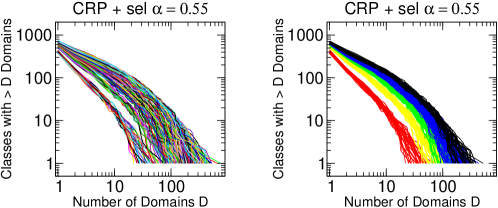
In order to identify model domain classes with empirical ones, it is necessary to label them. We assign each of the labels a positive or negative weight, according to its empirical frequency measured in figure 2C. A genome can then be assigned a cost function, according to how much its domain family compositions resembles the average one. In other words, the genome receives a positive score for every ubiquitous family it uses, and a negative one for every rare domain family. We then introduce a variant in the basic moves of the model, which can be thought of as a genetic algorithm. This variant proceeds as follows. In a first substep, the Chinese restaurant model generates a population of candidate genome domain compositions, or virtual moves. Subsequently, a second step discards the moves with higher cost, i.e. were specific domain classes sre used more differently from the average case. Note that the virtual moves could in principle be selected using specific criteria that keep into account other observed features of the data than the domain family frequency. The model is described more in detail in Supplementary Note S3. We mainly considered the case whith two virtual moves, which is accessible analytically.

In the modified model, not all classes are equal. The cost function introduces a significance to the index of the domain class, or a colored “tablecloth” to the table of the Chinese restaurant. In other words, while the probability distributions in the model are symmetric by switch of labels in domain classes Ald85 , this clearly cannot be the case for the empirical case, where specific folds fulfill specific biological functions. We use the empirical domain class usage to break the symmetry, and make the model more realistic. Moreover, the labels for domain classes identify them with empirical ones, so that the model can be effectively used as a null model.

Simulations and analytical calculations show that this modified model agrees very well with observed data. Figures 2B and 3B show the comparison of simulations with empirical data. The agreement is quantitative. In particular, the values of $\alpha$ that better agree with the empirical behavior of the number of domain classes as a function of domain size $F(n)$ are also those that generate the best slopes in the internal usage histograms $F(j,n)$. Namely, the best $\alpha$ are between 0.5 and 0.7. Furthermore, the cost function generates a critical value of $n$, above which $F(n)$, the total number of domain families, becomes flat. This behavior agrees with the empirical data better than the asymptotically growing laws of the standard CRP model. A mean-field calculation of the same style as the one presented above predicts the existence of this plateau (see Supplementary Note S3).

Discussion and Conclusions

The model shows that the observed common features in the number and population of domain classes organisms with similar proteome sizes can be explained by the basic evolutionary moves of innovation and duplication. This behavior can be divided into two distinct universal features. The first is the common scaling with genome size of the power laws representing the population distribution of domain classes in a genome. This was reported early on by Huynen and van Nimwegen HvN98 , but was not considered by previous models. The second feature is the number of domain families versus genome size $F(n)$, which clearly shows that genomes tend to cluster on a common curve. This fact is remarkable, and extends previous observations. For example, while it is known that generally in bacteria horizontal transfer is more widespread than in eukaryotes, the common behavior of innovation and duplication depending on coding genome size only might be unexpected. The sublinear growth of number of domain families with genome size implies that addition of new domains is conditioned to genome size, and in particular that additions are rarer with increasing size.

Previous literature on modeling of large-scale domain usage concentrated on reproducing the observed power-law behavior and did not consider the above-described common trends. In order to explain these trends we introduce a size dependency in the ratio of innovation to duplication $p_{N}/p_{O}$. This feature is absent in the model of Gerstein and coworkers, which is the closest to our formalism. We have shown that this choice is generally due to the fact that $p_{N}$ is conditioned by genome size. Furthermore, we can argue on technical grounds that the choice of having constant $p_{O}$ and $p_{N}$ would be more artificial, as follows. If one had $p_{0}^{i}=k_{i}/n$, the total probability $p_{O}$ would be one, since the total population $n$ is the sum of the class populations $k_{i}$, and there would not be innovation. In order to build up an innovation move, and thus $p_{N}>0$, one has to subtract small “bits” of probability from $p_{O}^{i}$. If $p_{N}$ has to be constant, the necessary choice is to take $p_{O}^{i}=k_{i}/n-p_{N}/f$, where $f$ is the number of domain classes in the genome. This means that the probability of duplication for a member of one class would be awkwardly dependent on the total number of classes. Furthermore, we have addressed the role of specificity of domain classes, by considering a second model where each class has a specific identity, given by its empirical occurence in the genomes of the SUPERFAMILY data set. This model, which gives up the complete symmetry of domain classes, gives the best quantitative agreement with the data, and is a good candidate for a null model designed for genome-scale studies of protein domains. More specific biological and physical properties, such as individual domain function and designability DS07 ; ZCS+07 ; OT05 come in at the more detailed level of description of how domains are actually used to form functional proteins.

It is useful to spend a few words on the role of common ancestry in these observations. Clearly, empirical genomes come from intertwined evolutionary paths, which determines their current states. On the other hand, the probability distributions predicted by the model are essentially the same for all histories (at fixed parameters), which can be taken as an idication that for these observations, the basic moves are more important than the shared evolutionary history. While the scaling laws are found independently on the realization of the Chinese restaurant model, the uneven presence of domain classes can be seen as strongly dependent on common evolutionary history. Averaging over independent realizations, the prediction of the standard model would be that the frequency of occurrence of any domain class would be equal, as no class is assigned a specific label. In the Chinese restaurant metaphor, the customers only choose the tables on the basis of their population, and all the tables are equal for any other feature. However, if one considers a single realization, which is an extreme, but comparatively more realistic description of common ancestry, the classes that appear first are obviously more common among the genomes. In the specific variant, the empirically ubiquitous classes are given a lower cost function, and tend to appear first in all realizations.

The next question worth discussing is the possible biological interpretation of the scaling of innovation to duplication, $p_{N}/p_{O}$ as a function of proteome size $n$. As we have shown, this ratio must scale in the correct way with $n$ in order to reproduce the data. As shown in table 1 and in figures 2 and 3, this is set by the parameter $\alpha$ of the model. Precisely, the ratio $p_{N}/p_{O}$ decreases like $\sim n^{\alpha-1}$. In other wirds necessarily something affects the addition of domains with new structures relative to domains with old structures, making it sparser with increasing size. This fact is not a prediction of the model, but rather a feature of the data, which constrains the model. Note that innovation events can have the three basic interpretations of horizontal transfers carrying new domain classes, gene-genesis or splitting of domain classes when internal structures diverge greatly, while duplication events can be interpreted as real duplication, or horizontal transfers carrying domains that belong to domain classes already present in the genome. While this might be confusing if one focuses on the genome, it seems reasonable to associate these processes to true “innovations” and “duplications” at the protein level. At least for bacteria, innovation by horizontal transfer could be the most likely event. In this case, the question could be reduced to asking why the relative rate of horizontal transfer of exogenous domain classes decreases with proteome size relatively to the sum of duplication and horizontal transfer of endogenous domain classes.

In order for $p_{N}/p_{O}$ to decrease with $n$, either $p_{O}$ has to increase, or $p_{N}$ has to decrease, or both. A possible source of increase of $p_{0}$ with $n$ is the effective population size. Recent studies LC03b suggest that coding genome size correlates with population size, and in turn this results in reduced selective pressure, allowing the evolution of larger genomes. Thus one can imagine that the ease to produce new duplications and proteome size are expected to correlate, purely on population genetics grounds. A naive reason for the innovation probability to decrease would be that the pool of total available domain shapes is small, which would affect the innovations at increasing size, while duplications are free of this constraint. However, this would imply that the currently observed genomes are already at the limit of their capabilities in terms of producing new protein shapes, while the current knowledge of protein folding does not seem to indicate this fact. On the other hand, the limited availability of domain classes could be true within a certain environment, where the total pool of domain families is restricted. We cannot exclude that the same kind of bias could be due to technical problems in the recognition and classification of new shapes in the process of producing the data on structural domains. If recognition algorithms tend to project shapes that are distinct on known ones, they could classify new shapes as old ones with a rate that increases with proteome size, leading to the observed scaling. Finally, we would like to suggest that a reason for $p_{N}$ to decrease with $n$ could be the cost for “wiring” new domains into existing interaction networks. The argument is related to the so-called “complexity hypothesis” for horizontal transfers JRL99 ; Ari05 ; LP08 ; WLG07 , which roughly states that the facility for a transferred gene to be incorporated depends on its position and status in the regulatory networks of the cell. We suppose that, given a genome with $n$ domains (or for simplicity monodomain genes) and $F$ domain families, the process leading to the acceptance of a new domain family, and thus to a new class of functions, will need a readaptation of the population of all the domain families causing an increase $\delta n$ in the number of genes. This increase is due to an underlying optimization problem that has to adapt the new functions exploited by the acquired family to the existing ones (by rewiring and expanding different interaction networks). To state it another way, we imagine that in order to add $\delta F$ new domain classes, or “functions”, it is necessary to insert $\delta n$ new degrees of freedom (“genes”) to be able to dispose of the functions. Now, generically, the computational cost for this optimization problem (which, conceptually, may be regarded as a measure of the evolvability of the system) could be a constant function of the size (and thus $\delta n\sim\delta F$), or else polynomial or exponential in $F$ (i.e. $\delta n\sim F^{d}\delta F$, where $d$ is some positive exponent, or $\delta n\sim\exp(F)\delta F$ respectively). Integrating these relations gives $n\sim F$ in the first case, $n\sim F^{d+1}$ in the second, and $n\sim\exp(F)$ in the third. Inverting these expressions shows that the first choice leads to the linear scaling of the model of Gerstein and coworkers, while the second two correspond to the CRP, and to a sublinear $F(n)$, which could follow a power law or logarithmic, depending on the computational cost. In other words, following this argument, accepting a new domain family becomes less likely with increasing number of already available domain families, as a consequence of a global constraint. This constraint comes from the trade-off between the advantage of incorporating new functions and the energetic or computational cost to govern them (both of which are related to selective pressure). This hypothesis could be tested by evaluating the rates of horizontal trasfers carrying new domain classes in an extensive phylogenetic analysis.

In conclusion, model and data together indicate that evolution acts conservatively on domain families, and show increasing preference with genome size to exploiting available shapes rather than adding new ones. A final point can be made regarding the number of observed domains. The model assumes that the new domain classes are drawn from an infinite family of shapes, which can be even continuous Pit02 , and leads to a discrete and small number of classes at the relevant sizes. Although physical considerations point to the existence of a small “menu” of shapes available to proteins BM07 , the validity of our model would imply that the empirical observation of a small number of folds in nature does not count as evidence for this thermodynamic property of proteins, but may have been a simple consequence of evolution.

We thank S. Maslov, H. Isambert, F. Bassetti, S. Teichmann, M. Babu, N. Kashtan and L.D. Hurst for helpful discussions.

$$\left.\begin{array}[]{c||l|l|l||l|l}&K_{i}&\frac{p_{N}}{p_{O}}&\frac{p_{N}}{p_{O}^{i}}&{\color[rgb]{1,0,0}F(n)}&{\color[rgb]{1,0,0}F(j,n)/F(n)}\\ \hline\cr\textrm{CRP }\alpha=0&\sim n&\sim n^{-1}&\sim n^{-1}&{\color[rgb]{1,0,0}\sim\log(n)}&{\color[rgb]{1,0,0}\sim\frac{\theta}{j}}\\ \textrm{CRP }\alpha>0&\sim n&\sim n^{\alpha-1}&\sim n^{\alpha-1}&{\color[rgb]{1,0,0}\sim n^{\alpha}}&{\color[rgb]{1,0,0}\sim j^{-(1+\alpha)}}\\ \textrm{Qian \emph{et al.} }&\sim n^{p_{O}}&=R&\sim n^{1-p_{O}}&{\color[rgb]{1,0,0}\sim n}&{\color[rgb]{1,0,0}\sim j^{-(2+R)}}\\ \end{array}\right.$$

Table 1: Salient features of the proposed model in terms of scaling of the number of domain classes, compared to the model of Gerstein and coworkers QLG01 ; KLQ+06 . The first three columns indicate the resulting average population of a class $K_{i}$, and the ratios of the probability to add a new class $p_{N}$ to the total and per-class probabilities of duplication, as a function of genome size $n$. These latter two quantities are asymptotically zero in the CRP, while they are constant or infinite in the model of Gerstein and coworkers. The last two columns indicate the resulting scaling of number of domain classes $F(n)$ and fraction of classes with $j$ domains $F(j,n)/F(n)$. The results of the CRP agree qualitatively with observations (i-iii) in the text.

Figure 1: Evolutionary Model. A. Scheme of the basic moves. A domain of a given class (represented by its color) is duplicated with probability $p_{N}$, giving rise to a new member of the same family (hence filled with the same color. Alternatively, an innovation move creates a domain belonging to a new domain class (new color) with probability $p_{N}$. B. Summary of the main mathematical quantities and parameters of the model.

Figure 2: Number of domain classes versus genome size. A. Plot of empirical data for 327 prokaryotes, 75 eukaryotes, and 27 archaeal genomes. Data refer to superfamily domain classes from the SUPERFAMILY database WMV+07 . Larger data points indicate specific examples. Data on SCOP folds follow the same trend (Supplementary Note S2). B. Comparison of data on prokaryotes (red circles) with simulations of 500 realizations of different variants of the model (yellow, grey, and green shade in the different panels), for fixed parameter values. Data on archaea are shown as squares. $\alpha=0$ (left panel, graph in log-linear scale) gives a trend that is more compatible with the observed scaling than $\alpha>0$ (mid panel). However, the empirical distribution of folds in classes is quantitatively more in agreement with $\alpha>0$ (see table 1 and figure 3). The model that breaks the symmetry between domain classes and includes specific selection of domain classes (right panel) predicts a saturation of this curve even for high values of $\alpha$, resolving this quantitative conflict. C. Usage profile of SUPERFAMILY domain classes in prokaryotes, used to generate the cost function in the model with specificity. In the x-axis, domain families are ordered by the fraction of genomes they occur in. The y-axis reports their occurrence fraction. The red lines indicate occurrence in all or none of the prokarotic genomes of the data set.

Figure 3: Internal usage of domains. A. Histograms of domain usage; empirical data for 327 prokaryotes. The x-axis indicates the population of a domain class, and the y-axis reports the number of classes having a given population of domains. Each of the 327 curves is a histogram referring to a different genome. The genome sizes are color-coded as indicated by the legend on the right. Larger genomes (black) tend to have a slower decay, or a larger cutoff, compared to smaller genomes (red). The continuous (red) and dashed (black) lines indicate a decay exponent of 3 and 1 respectively. B. Histograms of domain usage for 50 realizations of the model at genome sizes between 500 and 8000. The color code is the same as in panel A. All data are in qualitative agreement with the empirical ones. However, data at $\alpha=0$ appear to have a faster decay compared to empirical data. This is also evident looking at the cumulative distributions (Supplementary Note S1). The right panel refers to the model with specificity, at parameters values that reproduce well the empirical number of domain classes at a given genome size (figure 2). C. Population of the maximally populated domain class as a function of genome size. Empirical data of prokaryotes (green circles), are compared to realizations of the CRP, for two different values of $\alpha$, the lines indicate averages over 500 realizations, with error bars indicating standard deviation. $\alpha=0$ can reproduce the empirical trend only qualitatively (not shown). Data from the SUPERFAMILY databaseWMV+07 .

SUPPLEMENTARY NOTES

S1 Cumulative Distributions for the Internal Usage of Domains

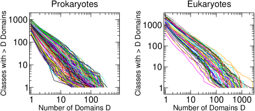
This section briefly discusses the cumulative histograms of domain usage for data and models. Figure S1.1 confirms the markedly power-law behavior observed for the histograms and predicted by the model. Comparison with the predictions of the CRP model (figure S1.2) shows faster decay for $\alpha=0$. While in good agreement with the observed number of domain classes with increasing size (figure 1B), this parameter choice is unsatisfactory on the quantitative side for the domain distribution in classes. This feature, already visible in figure 2B of the main text, is even more marked from the cumulative histograms. Better-fitting values are in the range $\alpha=0.5-0.7$. The CRP with specific domain classes (figure S1.3) has the same qualitative behavior as the standard model for the distributions, while fitting well the scaling of the classes of higher values of $\alpha$ (figure 1B and section S3 below).

Supporting Figure S1.1: Empirical cumulative distributions of domain usage for domain classes of the SUPERFAMILY database. The x-axis reports domain class sizes in number of domains $D$ while the y-axis refers to the histogram of the number of domain classes containing more than $D$ domains. The left panel is based on the same data on the 327 prokaryotes of figure 2A in the main text. The right panel refers to the 75 eukaryotes in the data set. The genome sizes are not color-coded to show individual plots.

Supporting Figure S1.2: Cumulative histograms of domain usage for 50 realizations of the CRP at genome sizes between 500 and 8000. Increasing values of $\alpha$ are plotted in lexicographic order.

Supporting Figure S1.3: Cumulative histograms of domain usage for 100 realizations of the CRP with specific classes at genome sizes between 1000 and 8000. In this size range the model variant produces essentially identical distributions to the conventional CRP, with better agreement on the growth in terms of domain classes (see section S3). The left panel is color-coded as figure 2B of the main text.

S2 Results for Fold Domain Classes

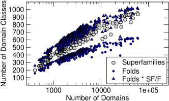
All data shown in the main text refer to the superfamily taxonomy level, and come from the SUPERFAMILY database. In this section, we report the results of the same analysis in terms of SCOP folds, which show that this category has essentially the same behavior as the previous one (figure S2.4). While by definition there are more superfamilies than folds, the number of domain classes versus genome size has very similar scaling in the two cases. The two plots collapse almost exactly, when folds are rescaled by the ratio (1443/884) of superfamilies per folds (S2.5). Furthermore, power-law fits of the experimental data for prokaryotes yield an exponent $\alpha$ between 0.3 and 0.4 for both categories, and logarithmic fits are also in agreement.

Supporting Figure S2.4: Top: Number of fold classes versus genome size, the plot is equivalent to figure 1A, except that the x-axis reports number of proteins scored in the genome, rather than genome size in domains. Since these two quantities are quite markedly linearly related, the two plots are equivalent. Bottom: histogram (left panel) and cumulative histogram (right panel) of domain classes for all genomes in the data set (eukaryotes, prokaryotes and archaea).

Supporting Figure S2.5: Comparison of the scaling of folds and superfamilies plot as a function of genome size. The plots refer to all genomes in the SUPERFAMILY database. The plot for folds (blue small circles) overlaps quite well with the plot for superfamily (large grey circles) when multiplied by the ratio of the total number of domain classes in the two taxonomies (1443/884).

S3 CRP Model with Specific Domain Classes and Analitycal Mean Field Equations

In this section we discuss the variant of the CRP model introduced in the main text and its analytical treatment. We first give some more details on the definition of the model. Generically, we consider the following genetic algorithm. For each genome size $n$, the configuration is a set of $M$ genomes $\{g_{1}(n),...,g_{M}(n)\}$, where each genome is a set of $D$ domain classes populated by some domains. An iteration is divided into two steps. A first “proliferation” step generates $qM$ genomes, where $q$ is a positive integer, $\{g^{{}^{\prime}}_{1}(n),...,g^{{}^{\prime}}_{qM}(n)\}$, using the standard CRP move. A second “selection” step discards the $(q-1)M$ individuals with higher cost.

Supporting Figure S3.6: Scheme of the CRP variant with domain specificity. At size $n$, multiple (two in the figure) “virtual” moves are generated with a standard CRP model, at fixed parameters. Subsequently, the moves with lowest cost (one in this case) are selected. In our case, the cost function is chosen by comparing the domain usage of the model genome with the empirical usage of specific domain families

The cost function, for a generic model genome $g$, can be a function $\mathcal{F}(g)$, that takes into account some phenomenological features observed in the data. We choose to include in $\mathcal{F}$ a minimal amount of empirical information on the occurrence of each domain class contained in figure 1C. In other words, we distinguish between “universal” domain classes, used in most of the genomes, and “contextual” ones, occurring only in a few examples. As discussed in the main text, this is sufficient to obtain quantitative agreement with the observed domain distributions (figures 1B and 2B), which are not given to the model as an input. If domain classes are indexed by $i=1..D$ ($D=1443$ for Superfamilies), we define the variable $\sigma^{g}_{i}$ as follows

$$\sigma^{l}_{i}=\left\{\begin{array}[]{cc}1&\textrm{if domain class }i\textrm{ is present in genome }g\\ -1&\textrm{if domain class }i\textrm{ is absent in genome }g\\ \end{array}\right.\ .$$

The cost function of that genome is then defined as

$$\mathcal{F}(g)=\exp\left(\sum_{i=1}^{D}\sigma^{g}_{i}\langle\sigma^{\mathrm{EMP}}_{i}\rangle\right)\ \ ,$$

where $\langle\sigma^{\mathrm{EMP}}_{i}\rangle$ is the empirical average of the same observable:

$$\langle\sigma^{\mathrm{EMP}}_{i}\rangle=\frac{1}{G}\sum_{g=1}^{G}\sigma^{g,\mathrm{EMP}}_{i}\ \ .$$

In the above formula $G$ is the number of observed genomes in the data set. For example, in the case of prokaryotes in the SUPERFAMILY database, $G=327$ and, calling $\Xi_{i}$ the function plotted in figure 1C, we have simply $\langle\sigma^{\mathrm{EMP}}_{i}\rangle=2\Xi-1$.

For the analitycal treatment, we considered the case $M=1$, $q=2$, where at each iteration, one genome is selected from a population of two. Starting from configuration $g(n)$, in the proliferation step genomes $g^{{}^{\prime}},g^{{}^{\prime\prime}}$ are generated with CRP rules, and the selection step chooses $g(n+1)=\mathrm{argmax}(\mathcal{F}(g^{{}^{\prime}}),\mathcal{F}(g^{{}^{\prime\prime}}))$. In this case, since the selection rule chooses strictly the maximum, it is able to distinguish the sign of $\langle\sigma^{\mathrm{EMP}}_{i}\rangle$ only. For this reason, it is sufficient to account for the positivity (which we label by “+”) and negativity (“-”) of this function for a given domain index $i$. The genomes $g^{{}^{\prime}}$ and $g^{{}^{\prime\prime}}$ proposed by the CRP proliferation step can have the same (labeled by “$1$”), lower (“$1_{+}$”) or higher (“$1_{-}$”) cost than their parent, depending on $p_{O}$, $p_{N}$ and by the probabilities to draw a universal or contextual domain family, $p_{+}$ and $p_{-}$ respectively. Using these labels, the scheme of the possible states and their outcome in the selection step is given by the table below.

$$\begin{array}[]{|c|c|c|}\hline\cr\textrm{proliferation }(g^{{}^{\prime}},g^{{}^{\prime\prime}})&\textrm{probability}&\textrm{selection}\\ \hline\cr(1,1)&p_{O}^{2}&\mathrm{old}\\ (1,1_{-})&2\>p_{O}\>p_{N}\>p_{-}&\mathrm{old}\\ \hline\cr(1,1_{+})&2\>p_{O}\>p_{N}\>p_{+}&\mathrm{new+}\\ (1_{+},1_{+})&p_{N}^{2}\>p_{+}^{2})&\mathrm{new+}\\ (1_{+},1_{-})&2\>p_{N}^{2}\>p_{-}\>p_{+}&\mathrm{new+}\\ \hline\cr(1_{-},1_{-})&p_{N}^{2}\>p_{-}^{2}&\mathrm{new-}\\ \hline\cr\end{array}$$

From this table, it is straightforward to derive the modified probabilities $\hat{p}_{O}$ and $\hat{p}_{N}$ of the complete iteration:

$$\hat{p}_{O}=p_{O}\>(p_{O}+2\>p_{N}p_{-})$$

$$\hat{p}_{N}=p_{N}\>(p_{N}+2\>p_{O}p_{+})=p_{N+}+p_{N-}\ \ ,$$

where $p_{N+}=p_{N}p_{+}(2-p_{N}p_{+})$ and $p_{N-}=p_{N}^{2}(1-p_{+})^{2}$ are the probabilities that the new domain is drawn from the universal or contextual families respectively.

We now write the macroscopic evolution equation for the number of domain families using the same procedure as in the main text. Calling $k^{+}(n)$ and $k^{-}(n)$ the number of domain classes that have positive or negative $\langle\sigma^{\mathrm{EMP}}_{i}\rangle$ and are not represented in $g(n)$,

$$\left\{\begin{array}[]{cc}\partial_{n}F(n)=&\hat{p}_{N}\\ \partial_{n}k^{+}(n)=&-\hat{p}_{N+}\\ \partial_{n}k^{-}(n)=&-\hat{p}_{N-}\\ \end{array}\right.\ .$$

Now, $p_{+}=k^{+}/(k^{-}+k^{+})=k^{+}/(D-F(n)$, so that we can rewrite

$$\left\{\begin{array}[]{cc}\partial_{n}F(n)=&(\frac{\alpha F(n)+\theta}{n+\theta})\>\Big{[}\frac{\alpha F(n)+\theta}{n+\theta}\>+\>\frac{2k^{+}(n)}{D-F(n)}(\frac{n-\alpha F(n)}{n+\theta})\Big{]}\\ \partial_{n}k^{+}(n)=&-(\frac{\alpha F(n)+\theta}{n+\theta})\>\frac{k^{+}(t)}{D-F(n)}\>\Big{[}2-\>(\frac{\alpha F(n)+\theta}{n+\theta})\frac{k^{+}(n)}{D-F(n)}\Big{]}\\ \partial_{n}k^{-}(n)=&-(\frac{\alpha F(n)+\theta}{n+\theta})^{2}\>(\frac{k^{+}(n)}{D-F(n)})^{2}\end{array}\right.$$ (1)

Supporting Figure S3.7: Numerical solutions of the mean-field equations of the CRP model with selection of specific domain classes. Left panel: cost function $\mathcal{F}(n)$ for different values of $\alpha$. Right panel: F(n) plotted in linear and logarithmic (inset) scales.

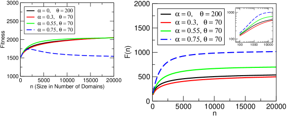
The above equations have the following consistency properties

• $\partial_{n}\Big{(}k^{+}+k^{-}+F\Big{)}=0$, hence $k^{+}+k^{-}+F=D\quad\forall n$.

• $\partial_{n}F\leq 1$, hence $F(n)\leq n$.

• $\partial_{n}F\geq 0$, $\partial_{n}k^{+}\geq 0$ and $\partial_{n}(F+k^{+})\geq 0$ so that $F$ grows faster than $k^{+}$ decreases.

Choosing the initial conditions from empirical data $n_{0},F(n_{0})$ size and number of domain classes of the smallest genome, we have, since $F(n_{0})<n_{0}$ and $\alpha\leq 1$,

$$\frac{\alpha F(n_{0})+\theta}{n_{0}+\theta}<1\ \ .$$

It is simple to verify that under this condition the system always has solutions that relax to a finite value $F_{\infty}<D$. Indeed, after the time $n^{*}$ where $k^{+}(n*)=0$, the equations reduce to $\partial_{n}k^{+}=0$, $k^{-}=D-F$ and

$$\partial_{n}F(n)=\left(\frac{\alpha F(n)+\theta}{n+\theta}\right)^{2}$$

immediately giving our result.

Numerical solutions of Eq. (1) give the same behavior for $F(n)$ as the direct simulations (figures S3.7A, and figure 2B of the main text). In particular, while this function grows as a power law for small genome sizes, it saturates at the relevant scale, giving good agreement with the data. This behavior is connected to the finite size of the pool of universal domain families, which we can interpret as the effect of a certain optimality in the core functions of the different organisms. The internal laws of domain usage of this model were obtained from direct simulations only, and, as discussed in the main text, give a more quantitative agreement with the data (figure 3B of teh main text). Finally, one interesting point can be made about the dynamics of the cost function. Figure S3.7B, shows that, for large values of $\alpha$ (above $0.7$) this function reaches a maximum at sizes between 2000 and 4000. This is also where most of the genomes in the data set are found, indicating that this range of genome sizes may allow the optimal usage of universal and contextual domain families.

S4 Other Variants of the CRP

We discuss here mean-field arguments for the robustness of our results on the asymptotics of $F(n)$ for two variants of the original model, including a small domain loss rate and global duplications.

Global Duplications.

One can consider the presence of global duplication moves. At each time step, if duplication is chosen, a number of domains selected with $q>1$ trials from a binomial distribution with parameter $p_{O}^{i}$ is duplicated in the same time step. The innovation step remains the same. In this case, it is not possible to measure time with the size $n$ of the genome, but this observable follows the evolution equation

$$\dot{n}=qp_{O}+p_{N}\ \ ,$$ (2)

where $\dot{\ }$ indicates the derivative with respect to time $t$. In terms of $t$, our mean field equations are worked out simply as $\dot{F}(t)=p_{N}$ and $\dot{K_{i}}(t)=qp_{O}^{i}$. Using Eq. (2), they can be simply converted in terms of $n$, yielding

$$\partial_{n}F(n)=\frac{\alpha F(n)+\theta}{qn+(q-1)\alpha F(n)+\theta}\ \ ,$$

and

$$\partial_{n}K_{i}(n)=\frac{K_{i}-\alpha}{n+\frac{\theta}{q}}\ \ .$$

The first equation gives as leading scaling $F(n)\sim n^{(\alpha/q)}$, showing that the growth of $F$ is pushed towards effectively lower values of $\alpha$ by global duplications, as a consequence of the rescaling of time by the global moves. The dynamics for $K_{i}$, instead, is affected only by a renormalization of the parameter $\theta$. The qualitative results of the model are therefore stable to the introduction of a global duplication rate, in the hypothesis that the extent of these duplications does not scale with $n$.

Supporting Figure S4.8: Number of domain classes with one member (related to $F(1,n)$) from the bacteria data set for superfamilies, plotted as a function of the number of domain classes (realted to $F$).

Domain Loss.

A second interesting variant of the model considers the introduction of a homogeneous domain deletion, or loss rate. Domain loss is known to occur in genomes. However, it is not considered in our basic model for simplicity and economy of parameters. In order to introduce it in the CRP, we define a loss probability $p_{L}=\delta$. This is equally distributed among domains, so that the per class loss probability is $p_{L}^{i}=\delta\frac{K_{i}}{n}$. Consequently, the duplication and innovation probability $p_{O}$ and $p_{N}$ are rescaled by a factor $(1-\delta)$. The mean-field evolution equation for the number of domain classes becomes then

$$\dot{F}(t)=(1-\delta)\frac{\alpha F+\theta}{n+\theta}-\delta\frac{F(1,n)}{n}\ \ ,$$

where the sink term for $F$ derives from domain loss in classes with a single element, quantified by $F(1,n)$.

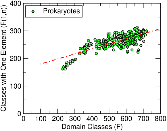
In order to solve this equation, one needs an expression for $F(1,n)$. Here, we report an argument based on the fact that in the empirical data, for large $n$, $F(1,n)=\gamma F(n)$, with $0<\gamma<1$ (figure S4.8). This is also confirmed by direct simulation of the model.

Using this experimentally motivated ansatz, we can show that for small $\delta$, the scaling of $F(n)$ is subject only to a small correction. Again, since time does not count genome size, one has to consider the evolution of $n$ with time $t$, given in this model simply by $\dot{n}=1-2\delta$. Using this equation it is possible to obtain the evolution equation for $F(n)$. Considering an expansion in small $\delta$ and large $n$, this reads to first order

$$\frac{\partial_{n}F(n)}{F(n)}=\frac{\alpha}{n}\left[1+\delta\left(\frac{\alpha-\gamma}{\alpha}\right)\right]\ \ .$$

The above equation gives the conventional scaling for $F(n)$, with the aforementioned correction. Note that the correction could be positive or negative, depending on the relative values of $\alpha$ and $\gamma$. An analogous argument holds for $\alpha=0$.

References

- (1) Orengo, C. A. & Thornton, J. M. Protein families and their evolution-a structural perspective. Annu Rev Biochem 74, 867–900 (2005).
- (2) Branden, C. & Tooze, J. Introduction to Protein Structure (Garland, New York, 1999).
- (3) Koonin, E. V., Wolf, Y. I. & Karev, G. P. The structure of the protein universe and genome evolution. Nature 420, 218–23 (2002).
- (4) Madan Babu, M. & Teichmann, S. Evolution of transcription factors and the gene regulatory network in Escherichia coli. Nucleic Acids Res 31, 1234–44 (2003).
- (5) Nye, T. M., Berzuini, C., Gilks, W. R., Babu, M. M. & Teichmann, S. A. Statistical analysis of domains in interacting protein pairs. Bioinformatics 21, 993–1001 (2005).
- (6) Qian, J., Luscombe, N. M. & Gerstein, M. Protein family and fold occurrence in genomes: power-law behaviour and evolutionary model. J Mol Biol 313, 673–81 (2001).
- (7) Ranea, J. A., Buchan, D. W., Thornton, J. M. & Orengo, C. A. Evolution of protein superfamilies and bacterial genome size. J Mol Biol 336, 871–87 (2004).
- (8) Murzin, A. G., Brenner, S. E., Hubbard, T. & Chothia, C. SCOP: a structural classification of proteins database for the investigation of sequences and structures. J Mol Biol 247, 536–40 (1995).
- (9) Orengo, C. A. et al. CATH–a hierarchic classification of protein domain structures. Structure 5, 1093–108 (1997).
- (10) Ranea, J. A., Sillero, A., Thornton, J. M. & Orengo, C. A. Protein superfamily evolution and the last universal common ancestor (LUCA). J Mol Evol 63, 513–25 (2006).
- (11) Bornberg-Bauer, E., Beaussart, F., Kummerfeld, S. K., Teichmann, S. A. & Weiner, J., 3rd. The evolution of domain arrangements in proteins and interaction networks. Cell Mol Life Sci 62, 435–45 (2005).
- (12) Weiner, J., 3rd, Beaussart, F. & Bornberg-Bauer, E. Domain deletions and substitutions in the modular protein evolution. FEBS J 273, 2037–47 (2006).
- (13) Huynen, M. A. & van Nimwegen, E. The frequency distribution of gene family sizes in complete genomes. Mol Biol Evol 15, 583–9 (1998).
- (14) Karev, G. P., Wolf, Y. I., Rzhetsky, A. Y., Berezovskaya, F. S. & Koonin, E. V. Birth and death of protein domains: a simple model of evolution explains power law behavior. BMC Evol Biol 2, 18 (2002).
- (15) Kuznetsov, V. A. In Zhang, W. & Shmulevich, I. (eds.) Computational and Statistical Approaches to Genomics, 125 (Kluwer, Boston, 2002).
- (16) Abeln, S. & Deane, C. M. Fold usage on genomes and protein fold evolution. Proteins 60, 690–700 (2005).
- (17) Wilson, D., Madera, M., Vogel, C., Chothia, C. & Gough, J. The SUPERFAMILY database in 2007: families and functions. Nucleic Acids Res 35, D308–13 (2007).
- (18) Li, H., Tang, C. & Wingreen, N. S. Are protein folds atypical? Proc Natl Acad Sci U S A 95, 4987–90 (1998).
- (19) Deeds, E. J. & Shakhnovich, E. I. A structure-centric view of protein evolution, design, and adaptation. Adv Enzymol Relat Areas Mol Biol 75, 133–91, xi–xii (2007).
- (20) Kamal, M., Luscombe, N., Qian, J. & Gerstein, M. Analytical Evolutionary Model for Protein Fold Occurrence in Genomes, Accounting for the Effects of Gene Duplication, Deletion, Acquisition and Selective Pressure. In Koonin, E., Wolf, Y. & Karev, G. (eds.) Power Laws, Scale-Free Networks and Genome Biology, 165–193 (Spinger, New York, 2006).
- (21) Durrett, R. & Schweinsberg, J. Power laws for family sizes in a duplication model. Ann. Probab. 33, 2094–2126 (2005).
- (22) Karev, G. P., Wolf, Y. I. & Koonin, E. V. Simple stochastic birth and death models of genome evolution: was there enough time for us to evolve? Bioinformatics 19, 1889–900 (2003).
- (23) Karev, G. P., Wolf, Y. I., Berezovskaya, F. S. & Koonin, E. V. Gene family evolution: an in-depth theoretical and simulation analysis of non-linear birth-death-innovation models. BMC Evol Biol 4, 32 (2004).
- (24) Karev, G. P., Berezovskaya, F. S. & Koonin, E. V. Modeling genome evolution with a diffusion approximation of a birth-and-death process. Bioinformatics 21 Suppl 3, iii12–9 (2005).
- (25) Dokholyan, N. V., Shakhnovich, B. & Shakhnovich, E. I. Expanding protein universe and its origin from the biological Big Bang. Proc Natl Acad Sci U S A 99, 14132–6 (2002).
- (26) Dokholyan, N. V. The architecture of the protein domain universe. Gene 347, 199–206 (2005).
- (27) Pitman, J. Combinatorial Stochastic Processes. In Notes for St. Flour Summer School (2002).
- (28) Pitman, J. & Yor, M. The two-parameter poisson-dirichlet distribution derived from a stable subordinator (1997).
- (29) Aldous, D. Exchangeability and related topics. In Saint-Flour Summer School XIII - 1983 (Springer, Berlin, 1985).
- (30) Kingman, J. Random discrete distributions. J. Roy. Statist. Soc. B 37, 1–22 (1975).
- (31) Barabasi, A. L. & Albert, R. Emergence of scaling in random networks. Science 286, 509–12 (1999).
- (32) Heijning, P., Scolari, V., Bassetti, B. & Cosentino Lagomarsino, M. Preprint.
- (33) Zeldovich, K. B., Chen, P., Shakhnovich, B. E. & Shakhnovich, E. I. A First-Principles Model of Early Evolution: Emergence of Gene Families, Species, and Preferred Protein Folds. PLoS Comput Biol 3, e139 (2007).
- (34) Lynch, M. & Conery, J. S. The origins of genome complexity. Science 302, 1401–4 (2003).
- (35) Jain, R., Rivera, M. C. & Lake, J. A. Horizontal gene transfer among genomes: the complexity hypothesis. Proc Natl Acad Sci U S A 96, 3801–6 (1999).
- (36) Aris-Brosou, S. Determinants of adaptive evolution at the molecular level: the extended complexity hypothesis. Mol Biol Evol 22, 200–9 (2005).
- (37) Lercher, M. J. & Pal, C. Integration of horizontally transferred genes into regulatory interaction networks takes many million years. Mol Biol Evol 25, 559–67 (2008).
- (38) Wellner, A., Lurie, M. N. & Gophna, U. Complexity, connectivity, and duplicability as barriers to lateral gene transfer. Genome Biol 8, R156 (2007).
- (39) Banavar, J. R. & Maritan, A. Physics of proteins. Annu Rev Biophys Biomol Struct 36, 261–80 (2007).