SPIN-08/033
ITP-UU-08/41
Scattering Amplitudes, Wilson Loops
and the String/Gauge Theory Correspondence
Luis F. Aldaya and Radu Roibanb
a Institute for Theoretical Physics and Spinoza Institute
Utrecht University, 3508 TD Utrecht, The Netherlands
b Department of Physics, Pennsylvania State University
University Park, PA 16802, USA
a l.f.alday@uu.nl, bradu@phys.psu.edu
We review, in a self-contained and pedagogical manner, recent developments and techniques for the evaluation of the scattering amplitudes of planar SYM theory at both weak and strong coupling. Special emphasis is placed on the newly discovered connection between a special class of amplitudes and the expectation values of particular cusped light-like Wilson loops.
(To be published in Physics Reports)
1 Introduction
There are two approaches to understanding and solving Yang-Mills (SYM): on the one hand, being a conformal field theory, it is uniquely specified by the spectrum of (anomalous) dimensions of gauge-invariant operators and their three-point correlation functions, while, on the other hand, like any other quantum field theory, it is completely specified by its scattering matrix.111In the presence of a regulator, the definition of the scattering matrix in a conformal field theory is no different than in any massive quantum field theory. The remarkable properties of SYM theory in the planar limit, in particular its high degree of symmetry, allowed important progress on both fronts: on the one hand, the integrability of the generator of scale transformations allows the evaluation of the anomalous dimensions of infinitely long operators through a Bethe ansatz Beisert:2005fw , Beisert:2006ib , BES while on the other hand the theory is sufficiently symmetric and with sufficiently good high energy behavior to allow high order perturbative calculations of its scattering matrix (see e.g.Bern:2007ct ).
The strong coupling regime of the theory is directly accessible through the AdS/CFT duality Maldacena:1997re , Gubser:1998bc , Witten:1998qj (see Aharony:1999ti for a review), which provides a description of SYM theory solely in terms of colorless, gauge invariant quantities. It casts the analysis of the strongly coupled planar theory in terms of the weakly-coupled worldsheet theory for superstrings in . Being in one to one correspondence with closed string states, local gauge invariant operators have a natural place in the AdS/CFT duality. This fact played a major role in our understanding of the spectrum of operators of the SYM theory (as well as in many other contexts).
Scattering amplitudes describe the scattering of on-shell states of the theory. As such, they carry color charge and thus it is not immediately clear whether they can be described directly by the closed string theory dual. It is however possible to extend the closed string theory in by an open string sector. Depending on the precise physical problem, they are described either by semiclassical worldsheet configurations (e.g. when they describe the expectation value of Wilson loops) or by vertex operators (e.g. when they capture the scattering amplitudes of open string states). Appropriately integrated, the correlation functions of open string vertex operators are what one might define as the gauge theory scattering amplitudes. Vertex operators carry Chan-Paton factors and the correlation functions of vertex operators decompose, in a natural way, into sum of terms, each of which exhibits a clean separation of the color degrees of freedom and the dependence on particle momenta. The factors carrying the kinematic dependence are known as partial amplitudes. This decomposition mirrors closely the color decomposition of gauge theory scattering amplitudes which we will discuss in section 2. While non-local quantities, partial amplitudes carry no color charge and thus could in principle be described by the closed string theory dual to SYM theory.
Strong coupling information extracted along these lines combined with weak coupling higher-loop calculations lead us to hope that, at least in some sectors, the scattering matrix of planar SYM theory can be found exactly. The four- and five-gluon amplitudes, which are currently known to all orders in perturbation theory (up to a set of undetermined constants), provide a proof of principle in this direction.
Here we review, in a self-contained and pedagogical manner, some of the recent developments and techniques for the evaluation of the scattering amplitudes of planar SYM theory at both weak and strong coupling. Related reviews of these topics may be found in references Dixon:2008tu , Alday:2008cg . The techniques developed for perturbative calculations in this theory have been extended to other less symmetric theories, as well as to QCD. For a detailed account we refer the reader to the original literature. We will however outline the attempts of generalizing the strong coupling arguments to other theories.
Section 2 is devoted to weak coupling calculations of scattering amplitudes. After setting up the notation and describing some of their general properties, we proceed to outline techniques for higher-loop high-multiplicity calculations. While the discussion is kept general at times, the main focus is planar SYM theory. The generalized unitarity-based method is the technique of choice for such calculations, as it combines in a natural way, order by order in perturbation theory, the consequences of global symmetries and of gauge invariance.
A common feature of all on-shell scattering amplitudes in massless gauge theories in four dimensions is the presence of infrared divergences, originating from low energy virtual particles as well as from virtual momenta almost parallel to external ones. We will discuss their structure captured by the soft/collinear factorization theorem. A surprising feature of certain planar amplitudes of SYM theory, noticed in explicit calculations, is that the exponential structure of the infrared divergences extends also to the finite part of the amplitude. We will describe the conjectured iteration relations based on this observations, which suggest that any maximally helicity violating loop amplitude may be written in terms of the corresponding one loop amplitude. We end section 2 with an outline of potential departures from these relations and the current state of the art in testing them.
For a variety of reasons, the identification and evaluation of the strong coupling counterpart of the partial amplitudes described in section 2 is not entirely straightforward. In section 3 we describe how the AdS/CFT duality can be used for this purpose. The main result is that, at strong coupling, partial amplitudes are closely related to a special class of polygonal, light-like Wilson loops. Thus, they may be evaluated as the area of certain minimal surfaces with boundary conditions fixed by the momenta of the massless particles participating in the scattering process.222Certain features of partial amplitudes – such as the polarization of the scattered particles – are however not captured directly by their Wilson loop interpretation. This information is best captured in the vertex operator picture for the scattering process. The strong coupling calculations exhibit features analogous to their weak coupling counterparts, such as the presence of long distance/low energy divergences. Thus, in analogy with the weak coupling situation, the very definition of scattering amplitudes requires the presence of a regulator. Finding gauge-invariant regulators is not completely obvious in weakly-coupled gauge theories; by contrast, any regulator which may be realized on the string theory side of the AdS/CFT correspondence without direct reference to the color degrees of freedom of the open string sector is manifestly gauge-invariant. To set-up the computation we begin by introducing a D-brane as an infrared regulator. Actual computations are, however, carried out using a string theory analog of dimensional regularization, obtained by taking the near horizon limit of D branes. While not yet clear how to extend the calculations beyond leading order, this regularization scheme has the advantage of being analogous to dimensional regularization as used in gauge theory calculations and thus of allowing a direct comparison of results.
We carry out the calculation of the four-gluon scattering amplitude both in the strong coupling version of dimensional regularization as well as using an infrared cut-off which removes, in a gauge-invariant way, all dangerous low energy modes. This cut-off scheme is particularly appropriate for understanding the conformal properties of the amplitudes at strong coupling.
The arguments used to construct the strong coupling interpretation of gluon partial amplitudes in SYM theory may be generalized to other, less symmetric theories and with a richer field content. We describe processes involving not only gluons but also local operators, mesonic operators and quarks. We end section 3 with an overview of other interesting discussions concerning the strong coupling limit of scattering amplitudes to leading and subleading orders.
While the arguments leading to it apply directly only in the strong coupling regime, the result – that the calculation of certain partial amplitudes is mathematically equivalent to the calculation of the expectation value of certain null polygonal Wilson loops – can be stated independently of the value of the coupling constant. This observation led to the conjecture that the same null polygonal Wilson loops reproduce maximally helicity violating (partial) amplitudes, order by order in weakly coupled perturbation theory. Section 4 reviews the evidence in favor of this conjecture, beginning with the explicit identification at one loop of the expectation value of the -sided null Wilson loop and the -gluon maximally helicity violating amplitude. This observation allows, as we will describe, for a direct strong coupling test of the BDS iteration relation described in section 2; the result suggests that the iteration relation needs to be modified in the strong coupling regime.
Unlike their generic counterparts, light-like Wilson loops are invariant under conformal transformations on the space they are defined on (in this case a space closely related to momentum space333In the case of SYM this space may itself be identified with the position space. In this formulation light-like Wilson loops are invariant under conventional conformal symmetry. Their expectation values may then be mapped back to momentum space and related to scattering amplitudes.). While the presence of divergences requires regularization, it can be argued that any regularization breaks this symmetry. The anomaly introduced by this breaking is an important tool for extracting higher-loop information on the expectation value of Wilson loops. Its key property is that it can be identified to all orders in perturbation theory due to its close relation to the structure of cusp singularities. We will review it in some detail in section 4. The resulting anomalous Ward identity mirrors the one discussed in section 3 at strong coupling. The restrictions imposed by conformal symmetry are particularly strong for Wilson loops corresponding to the scattering of a small number of particles, fixing uniquely the kinematic dependence of the expectation value of the four- and five-sided loop. We end section 4 by outlining the current state of the art in the calculation of expectation values of null polygonal Wilson loops, namely the two-loop expectation value of the four- and six-sided loop.
Partial amplitudes and (null polygonal) Wilson loops are a priori unrelated quantities. It is remarkable that a relation such as the one reviewed here can exist at all. Its origins and full implications remain to be uncovered; in section 5 we collect some open questions whose answers may lead to an improved understanding of the deep and powerful structures governing the dynamics of super-Yang-Mills theory and perhaps other four-dimensional gauge theories.
2 Scattering amplitudes at weak coupling
On-shell scattering amplitudes are perhaps the most basic quantities computed in any quantum field theory. The standard textbook approaches proceed to relate them through the LSZ reduction to Green’s functions which are in turn computed in terms of Feynman diagrams. Each diagram evaluated separately is typically more complicated that the complete amplitude; the reason may be traced to Feynman diagrams not exhibiting and taking advantage of the symmetries of the theory – neither local nor global. The first instance where this shows up is for tree level amplitudes, where one notices major simplifications as all diagrams are added together.
Indeed, besides the scattering of physical polarizations, off-shell scattering amplitudes also describe the scattering of (unphysical) longitudinal polarizations of vector fields. On-shell, the equations of motion (or, more generally, Ward identities) guarantee the decoupling of such states. One may expose this decoupling at the Lagrangian level by choosing a physical gauge. The resulting gauge-fixed action does not, however, have a transparent use at the quantum level. As usual, in an off-shell covariant and renormalizable approach to loop corrections to scattering amplitudes, Faddeev-Popov ghosts are needed to cancel the contribution of unphysical fields propagating in loops.
The (generalized) unitarity-based method provides means of eliminating the appearance of unphysical degrees of freedom, while preserving all on-shell symmetries of the theory and avoiding the proliferation of Feynman diagrams. It allows the analytic construction of loop amplitudes in terms of tree-level amplitudes. Thus, it manifestly incorporates most (if not all) simplifying consequences of gauge invariance and symmetries. Simplicity of loop level amplitudes is to a large extent a consequence of simplicity of tree-level amplitudes.
In addition to the use of Feynman diagrams, there are several methods for computing tree-level scattering amplitudes: the Berends-Giele (off-shell) recursion relations Berends_Giele , MHV vertex rules CSWrules 444The MHV vertex rules have been successfully extended to loop level in BST . and the BCFW recursion relations BCFW1 , BCFW2 . We will not review them in detail and refer the reader to the original literature and existing reviews Dixon_TASI , Bern:2007dw , Cachazo_Svrcek . Instead, we will be focusing on the construction of loop amplitudes, assuming that the tree-level amplitudes are known. After setting up the convenient notation and describing some of the general properties of scattering amplitudes, we will review the factorization of infrared divergences, discuss the unitarity method and illustrate it with several examples. We will then describe the BDS conjecture for the all-loop resummation of -point MHV amplitudes, the potential corrections and the fact that such corrections indeed appear starting with the six-point two-loop amplitude. We will also describe the emergence of dual conformal invariance from the explicit expressions of amplitudes.
2.1 Organization, presentation and general properties
A good notation as well as an efficient organization of the calculation and result are indispensable ingredients for the calculation of scattering amplitudes, whether with Feynman diagrams or by other means. They are provided, respectively, by the spinor helicity method (for massless theories) and by color ordering, which we now review. These methods allow the decomposition of amplitudes in smaller, gauge-invariant pieces with transparent properties. An enlightening discussion of these topics may be found in Dixon_TASI .
2.1.1 Spinor helicity and color ordering
In a massless theory, solutions of the chiral Dirac equation provide an excellent parametrization of momenta and polarization vectors which allows, among other things, the construction of physical polarization vectors without fixing noncovariant gauges. The main observation is that the sum over polarizations of a direct product of a Dirac spinor and its conjugate is
| (2.1) |
Upon projecting onto the chiral components one immediately finds that
| (2.2) |
where as usual are the Pauli matrices. The decomposition of a massless four-dimensional vector as a direct product of two 2-component commuting “spinors” follows also more formally from the fact that , implying that the mass-shell condition requires that has unit rank, i.e.
| (2.3) |
the multiplication of spinors follows from Lorentz invariance:
| (2.4) |
In Minkowski signature and are complex conjugate of each other. It is useful to promote momenta to (holomorphic) complex variables and the Lorentz group to . Then, and are independent complex variables and the decomposition (2.3) exhibits a scaling invariance
| (2.5) |
where is an arbitrary constant. We will shortly see that scattering amplitudes have definite scaling properties under this transformation.555For a Minkowski signature metric is a pure phase.
This parametrization of four-dimensional momenta allows the construction of simple expressions for the physical polarizations of massless vector fields. In general, gauge invariance requires that they be transverse, and that shifts by the momentum of the corresponding field should not change their form and properties. Moreover, in the frame in which the vector field propagates along a specified axis, they should take the standard form of circular polarization vectors.
A solution to these constraints can be constructed in terms of an arbitrary null (reference) vector ():
| (2.10) |
The reference vector may be changed by a gauge transformation. Indeed, the transformation for some can be realized as a change of the reference vector:
| (2.11) |
This freedom of choosing independently the reference vector for each of the gluons participating in the scattering process is a very convenient tool for simplifying (somewhat effortlessly) the expressions for (tree-level) scattering amplitudes.
The loop expansion of scattering amplitudes is defined in the usual way:
| (2.12) |
A clean organization of scattering amplitudes is a second useful ingredient in the calculation of scattering amplitudes at any fixed loop order . Besides the organization following the helicity of external states implied by spinor helicity, at each loop order an organization following the color structure is also possible and desirable, if only because amplitudes are separated in at least gauge invariant pieces (here is the number of external legs). For an gauge theory with gauge group generators denoted by , it is possible to show that any -loop amplitude may be decomposed as follows:
| (2.13) |
where the sum extends over all non-cyclic permutations of . This is equivalent to fixing one leg – say the first – and summing over all permutations of the other legs. The coefficients are called color-ordered amplitudes. The multi-trace terms left unspecified in the equation above do not appear in the planar (large ) limit, which will be our main focus. We shall therefore ignore them in the following. In the same limit the dependence of the partial amplitudes drops out:
| (2.14) |
The latter are the so called planar partial amplitudes, while the subleading terms in the expansion as well as the multi-trace terms in (2.13) are called non-planar partial amplitudes.
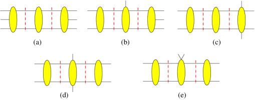
It is possible to argue for this presentation of amplitudes by inspecting the Feynman rules and noting that their color dependence separates from their momentum dependence. Perhaps the cleanest argument however is in terms of string theory diagrams Bern_Kosower_1991 . Indeed, in string theory, gluon scattering amplitudes are computed in terms of Riemann surfaces with boundaries. Vertex operators carrying Chan-Paton factor are inserted on their boundaries, with color indices contracted along boundaries (see figure 1). As one integrates over the insertion points one sweeps over all possible orders of inserting the operators. The cyclic permutations however are naturally excluded because the boundaries in question are closed curves. The boundaries carrying no vertex operators contribute the explicit factors of in equation (2.13).
2.1.2 General properties of color ordered amplitudes
The general properties of color-ordered amplitudes follow from their construction in terms of Feynman diagrams (or string diagrams). The results of other constructions must obey the same properties. Some of them – such as the analytic structure – impose powerful constraints and in some cases uniquely determine the (tree-level) amplitudes. We collect here some of the more important properties Mangano_Parke_Xu :
-
•
cyclicity (this is a consequence of the cyclic symmetry of traces)
(2.15) -
•
reflection (this is a consequence of the fact that 3-point vertices pick up a sign under such a reflection and that an amplitude with external legs has three-point vertices)
(2.16) -
•
photon decoupling: In a theory with only adjoint fields, the diagonal does not interact with anyone. Thus, all amplitudes involving this field identically vanish. At tree-level this property may be captured by a Ward identity: fixing one of the external legs ( below) and summing over cyclic permutations of the remaining legs leads to a vanishing result:
(2.17) In string theory language this is a consequence of the structure of the operator product expansion of vertex operators. At loop level this identity is modified and relates planar and nonplanar partial amplitudes Bern_Kosower_1991 .
-
•
parity invariance (a color-ordered amplitude containing all choices of helicities of external legs is invariant if all helicities are reversed and simultaneously all spinors are replaced by the spinors and vice-versa). This operation may be expressed as a fermionic Fourier-transform RSV_2
(2.18) -
•
soft (momentum) limit: in the limit in which one momentum becomes soft the amplitude universally factorizes as follows
(2.19) -
•
collinear limit: in the limit in which two adjacent momenta become collinear an -loop amplitude factorizes as
(2.20) where denotes the helicity of the -th gluon. For a given gauge theory, the -loop splitting amplitudes are universal functions Kosower_splitting of the helicities of the collinear particles, the helicity of the external leg of the resulting amplitude and of the momentum fraction defined as
(2.21) In the strict collinear limit one may also use and with . For example, the tree-level splitting amplitudes are:
(2.22) In SYM theory Ward identities imply that all splitting amplitudes rescaled by their tree-level expressions are the same.
Scattering amplitudes have similar factorization properties when more than two adjacent momenta become simultaneously collinear Kosower_splitting .
-
•
multi-particle factorization: color ordered amplitudes exhibit poles if the square of the sum of some adjacent momenta vanishes. At tree-level this pole corresponds to some propagator going on-shell. At higher loops, the amplitude decomposes into a completely factorized part given by the sum of products of lower loop amplitudes and a non-factorized part, given in terms of additional universal functions. At one-loop level and in the limit one finds Bern_Chalmers
(2.23) (2.24)
While color ordering (2.13) in the planar theory implies that complete amplitudes may be reconstructed from gauge invariant partial amplitudes, the first four properties listed above imply that only a much smaller number is in fact necessary.
2.1.3 Some simple examples
Besides color ordering, scattering amplitudes can be organized following the number of negative helicity gluons. One can easily see that the amplitude with only positive helicity gluons as well as the amplitude with a single negative helicity gluons vanish identically at tree level in any gauge theory. This is realized by choosing the same reference vectors for all gluons with the same helicity and equal to the momentum of the negative helicity gluon. In absence of supersymmetry, quantum corrections spoil this conclusion. In the presence of supersymmetry, its Ward identities imply that this vanishing result is protected to all orders in perturbation theory. Indeed, the supersymmetry transformation rules are
| (2.26) | |||
where is a reference spinor. Acting with them on the vanishing matrix element and using the fact that fermions have only helicity-conserving interactions, it immediately follows that the all-plus amplitude vanishes. Similarly, using the vanishing of and making judicious choices for the reference spinor leads to the vanishing of the amplitude with a single negative helicity gluon Grisaru:1977px 666To spell out the details, we use an part of the supersymmetry algebra and denote by the gaugino related to the gluon by these transformations: implies the vanishing of the all-plus amplitude while immediately implies, after choosing , the vanishing of the amplitude with a single negative helicity gluon.
| (2.28) |
In the following we will focus mainly on SYM.
The first nonvanishing amplitude, having two negative helicity gluons, takes the form Parke_Taylor1 , Parke_Taylor2
| (2.29) |
where is a cyclic index (i.e. ) and and are the labels of the negative helicity gluons. The fact that in SYM the two gluon helicity states are related by supersymmetry makes it possible to show Bern:1996ja that, to all loop orders, -point MHV amplitudes are cyclicly symmetric, up to an overall factor of where and label, as above, the negative helicity gluons. Indeed, using supersymmetric Ward identities it is possible to relate the -gluon amplitude to the two scalar, -gluon amplitude. After interchanging the position of the two scalars, which does not affect the amplitude, one may use the same identities to obtain an amplitude with one of the two negative helicity gluons displaced to any position. It thus follows that, to any loop order ,
| (2.30) |
where is a cyclicly symmetric function of momenta and . This factorization of the tree-level amplitude also holds for the infrared-singular terms of all amplitudes in all massless gauge theories. A similar expression holds in SYM also for collinear splitting amplitudes introduced in (2.20):
| (2.31) |
where the momentum fraction is defined in equation (2.21). A direct argument follows closely the one for MHV amplitudes. Alternatively, one may extract it by simply comparing the collinear limit of (2.30) and the expected behavior (2.20).
2.1.4 Soft/Collinear factorization
A general feature of massless gauge theories in four dimensions is the existence of infrared singularities.777Ultraviolet divergences may of course be present as well; as previously mentioned, our focus is SYM theory, which is free of such divergences. Unlike ultraviolet divergences they cannot be renormalized away, but rather should cancel once gluon scattering amplitudes are combined to compute infrared-safe quantities. Their structure has been thoroughly studied and understood (see e.g. IR_paper1 , IR_paper2 , IR_paper3 , IR_paper4 , IR_paper5 , IR_paper6 , IR_paper7 , IR_paper8 , IR_paper9 , IR_paper10 , IR_paper11 , IR_paper12 , AM2 ). Here we briefly review some of the results specializing them, following Bern:2005iz , to the case of SYM in the planar limit.
In a gauge theory, infrared singularities of scattering amplitudes come from two sources: the small energy region of some virtual particle
| (2.32) |
and the region in which some virtual particle is collinear with some external one
| (2.33) |
Since they can occur simultaneously, at -loops the infrared singularities lead to an pole.
The structure of soft and collinear singularities in a massless gauge theory in four dimensions has been extensively studied. The realization that soft and virtual collinear effects can be factorized in a universal way, together with the fact Collins_Soper_Sterman that the soft radiation can be further factorized from the (harder) collinear one led to a three-factor structure for gauge theory scattering amplitudes Sen:1982bt , Sterman:2002qn , MertAybat:2006mz :
| (2.34) |
Here the product runs over all the external lines. is the factorization scale, separating soft and collinear momenta, is the renormalization scale and is the running coupling at scale . Both and the rescaled amplitude are vectors in the space of color configurations available for the scattering process. The soft function is a matrix acting on this space and it is defined up to a multiple of the identity matrix. It captures the soft gluon radiation and it is responsible for the purely infrared poles. For this reason it can be computed in the eikonal approximation in which the hard partonic lines are replaced by Wilson lines. The “jet” functions do not alter the color flow and contain the complete information on collinear dynamics of virtual particles. Finally, contains the effects of highly virtual fields and is finite as . The jet and soft functions can be independently defined in terms of specific matrix elements.
The factorization scale is arbitrary (within some physical limits); it is simply used to construct the equation (2.34). While it enters in each of the three factors on the right hand side, the (rescaled) amplitude is independent of it. This independence, akin to the independence on the renormalization scale , leads to a evolution equation for the soft function.
In the planar limit the soft/collinear factorization formulae simplify significantly. Since in this limit there is a single color structure, all color-space vectors reduce to a single component. The fact that the soft function is defined only up to an overall function implies that, in the planar limit, it can be completely absorbed in the jet functions . The planar limit implies that all interactions included in the thus redefined jet functions are confined to adjacent gluons. In this limit it is then instructive to consider a two-gluon process – simply the decay of a color-singlet state into two gluons. Direct application of the factorization equation identifies then the square of the jet function with the amplitude of this process which is, by definition, the Sudakov form factor if the two gluons have momenta and . It therefore follows that, in the planar limit, a generic -point scattering amplitude factorizes as
| (2.35) |
where is the ’t Hooft coupling. As before, here denotes a generic resummed amplitude, rescaled by the corresponding tree-level amplitude.
Similarly to the soft and jet functions, the factorization (2.35) implies an evolution equation and a renormalization group equation for the factors . The same equations follow independently from the gauge invariance and the properties of the form factor. They read
| (2.36) |
where the function contains only poles and no scale dependence. The functions and themselves obey renormalization group equations IR_paper2 , IR_paper3 , IR_paper4 , Ivanov:1985np , Korchemsky:1985xj
| (2.37) |
In SYM they may be solved exactly and explicitly in terms of the expansion coefficients of the cusp anomalous dimension
| (2.38) |
and another set of coefficients defining the expansion of :
| (2.39) |
where the coupling constant customarily used in higher loop calculations. An important ingredient in solving these equations is that in the dimensionally-regularized SYM theory the beta function is
| (2.40) |
i.e. in the presence of the dimensional regulator the theory is infrared-free. The solution for and may then be used to reconstruct the Sudakov form factor (2.36) which, in turn, leads to the following expression for the factorized amplitude Bern:2005iz :
| (2.41) | |||||
| (2.42) |
The definition of may be easily seen to be
| (2.43) |
This function captures the divergences of the planar one-loop -point amplitudes in SYM.
The first few coefficients in the weak coupling expansion of the cusp anomalous dimension and function (2.39) have been evaluated directly CuspWeak , Belitsky:2003ys , Bern:2005iz , Kotikov_1 , Kotikov_2 , BCDKS , CSVcusp , CSVcollinear with the result
| (2.44) | |||||
| (2.45) |
Using the integrability of the gauge theory dilatation operator BES constructed an integral equation whose solution is the universal scaling function (conjecturally equal to the cusp anomalous dimension) to all orders in perturbation theory. This equation was solved in a weak coupling expansion BES and also in a strong coupling expansion BKK1 , BKK2 , BKK3 . Using the AdS/CFT correspondence the first few coefficients in the strong coupling expansion were evaluated in CuspStrongCoupling1 , CuspStrongCoupling2 , CuspStrongCoupling3 . The leading term in the strong coupling expansion of was computed in AM1 :
| (2.46) | |||||
| (2.47) |
here is the Catalan constant.
The properties of the collinear anomalous dimension were discussed in detail in Dixon_Magnea_Sterman where this function was identified with the sum of the first subleading term in the large spin expansion of the anomalous dimension of twist-2 operators and the coefficient of the subleading pole in the expectation value of the cusp Wilson line with edges of finite length.
2.2 Loop amplitudes; generalized unitarity-based method
Having discussed general properties of scattering amplitudes, we now proceed to describe methods for their construction at loop level. The goal will be to use only on-shell information for this purpose. we will be assuming (quite accurately) that tree-level amplitudes are known. As we will see, the fact that Feynman diagramatics underlies the calculation of scattering amplitudes is a very important and useful guide. The properties of color ordered amplitudes discussed previously will serve as a useful guide for the completeness of the result. While most arguments apply to any (supersymmetric) gauge theory, we will be having in mind applications to SYM.
The idea that one can use only on-shell information to construct loop-level scattering amplitudes is of course very appealing. For starters, one would use complete lower-loop amplitudes as building blocks of higher amplitudes and, as such, one would build in the calculations simplifications due to symmetries and gauge invariance.
There is a long history associated with on-shell methods going back to the time of the analytic S-matrix theory. The idea is that, given the discontinuity of the amplitude in some channel – or a cut – one could use a dispersion integral to reconstruct the complete amplitude. In turn, the discontinuity of amplitudes is determined by the unitarity condition of the scattering matrix. Indeed, separating the interaction part of the scattering matrix
| (2.48) |
and requiring that is unitary implies that
| (2.49) |
The right hand side is the product of lower loop on-shell amplitudes; this may be interpreted as a higher loop amplitude with some number of Feynman propagators replaced by on-shell (or “cut”) propagators
| (2.50) |
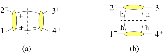
The difference on the left hand side of equation (2.49) is interpreted as the discontinuity in the multi-particle invariant obtained by squaring the sum of the momenta of the cut propagators. This interpretation is a consequence of the prescription. Thus, this discontinuity at -loops is determined in terms of products of lower-loop amplitudes. There are two types of cuts: singlet and non-singlet. In the former only one type of field crosses the cut. In the latter several types of particles (such as a complete multiplet in a supersymmetric theory) cross the cut. For the one-loop four-gluon amplitude this is illustrated in figure 3; in figure 3(a) the tree-level amplitudes require that only gluons can propagate along the cut propagators while in figure 3(b) fields with any helicity can cross the cut, i.e. .
Having determined it, the missing (real) part of the amplitude is constructed from a dispersion integral:
| (2.51) |
where is the momentum invariant flowing across the cut. The term coming from the contour at infinity vanishes if as . If it does not, there are subtraction ambiguities related to terms which have no discontinuities. The first string scattering amplitudes at one-loop were evaluated through such a method KSV , BHS .
While perfectly valid, such an approach does not make use of recent sophisticated techniques for evaluating Feynman integrals: identities, modern reduction techniques, differential equations, reduction to master integrals, etc. A reinterpretation of the equation (2.49) leads however in this direction. Indeed, besides representing the discontinuity of the amplitude, the right-hand-side of that equation also represents the part of the amplitude which contains the cut propagators. In fact, the right hand side of that equation contains a combination of parts of the amplitude containing two, three up to propagators.
It is not hard to see that separately each of these pieces are given by products of on-shell lower-loop amplitudes. This conclusion may be reached by thinking of the complete amplitude from a Feynman diagram perspective. Consider looking at the part of the amplitude which contains some prescribed set of propagators such that if they are cut the amplitude falls apart in at least two disconnected pieces. Since the full amplitude is a sum of Feynman diagrams, each of the resulting pieces it itself a sum over all Feynman diagrams having as external legs (some) of the original external legs as well as (some of) the cut lines. Thus each of the resulting parts is itself an on-shell amplitude, with the on-shell condition being a consequence of the cut conditions (2.50).
This observation, originally due to Bern, Dixon, Dunbar and Kosower BDDK_npt and improved at one-loop level in BCF_unitarity , allows to “cut” more than propagators for an -loop amplitude, generalizing the unitarity relation (2.49). Similarly to regular cuts, generalized cuts can be either of singlet and nonsinglet types. These properties open the possibility of going beyond reconstructing the amplitudes from dispersion integrals: instead, one identifies the pieces of an amplitude with some prescribed set of propagators. Analyzing sufficiently many combinations of propagators one is guaranteed to be able to reconstruct the complete amplitude. Indeed, the fact that Feynman rules express scattering amplitudes as a sum of terms containing propagators and vertices implies that, after integral reduction, each term in the result contains part of the propagators present in the initial Feynman diagrams. By analyzing all possible generalized cuts one probes all possible combinations of propagators and thus all possible terms originating from the Feynman diagrams underlying the scattering process.
The argument above assumes that the (generalized) cuts are constructed in the regularized theory – i.e. in -dimensions (perhaps with ). In practice however it is much simpler to start by analyzing four-dimensional cuts, as one can saturate them with four-dimensional helicity states and also make use of the simplifying consequences of the supersymmetric Ward identities, such as (2.28). Four-dimensional cuts however potentially miss terms arising from the -dimensional components of the momenta in the momentum-dependent vertices. Such terms must be separately accounted for (either by considering -dimensional cuts or by other means). In supersymmetric theories one can argue BDDK_cut_constructibility , based on the improved power-counting of the theory, that at one-loop level such terms do not exist through (in the sense that through one-loop amplitudes follow from four-dimensional cut calculations).
Let us illustrate this discussion with a simple example – that of the four gluon scattering amplitude in SYM. We will organize the calculation in terms of regular, two-particle cuts reinterpreted in the spirit of generalized unitarity-based method. There are two cuts – in the and in the -channels. Depending upon the external helicity configuration either one or both cuts are of non-singlet type, with the complete supermultiplet crossing it. As discussed previously, the helicity information in any MHV amplitude (such as this one) is carried by an overall factor of the tree-level amplitude (2.30). The remaining function may be thus computed by choosing the most convenient helicity configuration. Choosing and evaluating the four-dimensional -channel cut (figure 3(a)) one finds without difficulty that
| (2.52) |
Here and we have used the fact that the cut condition allows one to write . In the propagator-like structures one recognizes the cut of a scalar box integral in theory (that is, the integrand of a box integral in theory in which two propagators have been removed and the on-shell condition for the corresponding momenta is imposed). At this stage one can argue based on the ultraviolet behavior of SYM that the full answer is given by the box integral whose -channel cut we have just computed. Indeed, any other scalar integral diverges in a smaller number of dimensions than SYM and thus cannot appear in the final result. The conclusion of this argument can be confirmed by the evaluation of the (nonsinglet) -channel cut (figure 3(b)). The simplest way to see this is to make use again of the equation (2.30) and note that up to the tree-level factor, the -channel cut in the configurations and are the same. The latter is again a singlet cut, being given by a relabeling of equation (2.52). To summarize, we find BDDK_npt that
| (2.53) |
thus reproducing the well-known result of GreenSchwarz .
The fact that a scalar box integral appears in the result of this calculation is not surprising. On general grounds one can show that in any four-dimensional massless theory, any one-loop scattering amplitude may be expressed as a linear combination of scalar box, triangle and bubble integrals (i.e. integrals with four, three and two propagators, respectively, and no loop-momentum factors appearing in the numerator) with rational coefficients (see figure 4) and a rational function which has no cuts in any channel. It was shown in BDDK_npt that in a supersymmetric theory this rational contributions are absent and that in such theories one-loop amplitudes are constructible using four-dimensional cuts.

For one-loop amplitudes in SYM one can do much better than the above by noticing BDDK_npt that the one-loop amplitudes with external states belonging to the same vector multiplet may be written as a sum of box integrals. Besides a massless box integral which occurs only for four-gluon scattering, these integrals fall in five different classes: one-mass, easy two-mass, hard two-mass, three- and four-mass box integrals, depending on whether massive or massless momenta are injected at the corner of the box. The first two classes are shown in figure 5. The box integrals are defined and given in ref. bdk_integrals_1 , bdk_integrals_2 (the four-mass boxes are from ref. denner , davydychev_1 , davydychev_2 ). Since each box integral has a unique set of four propagators (cf. figure 4), a quadruple cut (i.e. the result of eliminating four propagators and using the on-shell condition for their momenta) isolates a unique box integral and its coefficient BCF_unitarity . The quadruple cut of the amplitude is, following the previous discussion, simply given by the product of four tree amplitudes evaluated on the solution of the on-shell conditions for the four propagators. Thus:
| (2.54) |
where the labels are cyclic indices and label the first external leg at each corner of the box, counting clockwise. The sum runs over all possible helicity assignments on the internal lines. The factor of above is due to the four on-shell conditions having two solutions with equal values of the quadruple-cut box integrals are equal. The sum over these solutions is implicit in the sum in equation (2.54). An implicit assumption is made in writing this expression. Any amplitude contains at least one box integral with one three-point corner. In Minkowski signature – i.e. with real momenta – the corresponding tree-level three-point amplitude vanishes identically. A nonvanishing result requires interpreting the loop momentum as complex.
We will later need the expression for the one-loop MHV amplitude. As we discussed, the four-point amplitude is given by (. For an arbitrary number of external legs (larger than four), the result initially obtained in BDDK_npt (which can be reproduced using quadruple cuts and complex momenta) reads:
| (2.55) | |||||
| (2.57) | |||||
where and are the one-mass (figure 5(a)) and easy two-mass (figure 5(b)) integrals and are multi-particle invariants . 888This is a more compact notation for ..

2.3 Calculations at higher loops
Higher loop calculations in SYM enjoy similar simplifications, though to a lesser extent. An analog of the 1-loop integral basis is not available, in the sense that the members of all proposed bases are in fact functionally dependent integrals 999Notable examples are the two-loop four-point integral basis with massless external legs Smirnov_Veretin and the two-loop four-point integral basis with one massive external leg Gehrmann_Remiddi .; moreover, not all integrals have sufficiently many propagators such that the cut condition on all of them does not completely freeze the integrals. It was pointed out Buchbinder_Cachazo that under certain circumstances, after all propagators have been set on-shell, an additional propagator-like structure appears which can be used to set an additional on-shell condition. The lack of independence of the integral basis does not allow however a straightforward identification of the resulting product of tree amplitudes with the coefficient of the integral which is isolated by these cuts.
Generalized cuts can nevertheless be used to great effect to isolate parts of the full amplitude containing some prescribed set of propagators. One needs to ensure that integrals are not double-counted and that all cuts are consistent with each other. The previous arguments continue to hold and imply that the complete amplitude can be reconstructed from its -dimensional generalized cuts. A detailed, general algorithm for assembling the amplitude was described in QCD_splitting_amplitude . In a nutshell, starting from one (generalized) cut, one corrects it iteratively such that all the other cuts are correctly reproduced.
While fundamentally all cuts have equal importance, some of them exhibit more structure, which makes them ideal starting points for the reconstruction of the amplitude. Such are the iterated two-particle cuts, defined as a sequence of two-particle cuts which at each stage reduces the number of loops by one unit.101010It is fairly clear that a priori there exist integrals which do not exhibit any two-particle cuts. Such contributions to the amplitude are not captured in this way. An example is provided by the four-loop four-gluon planar amplitude BCDKS . Their importance stems from the fact that two-particle cuts with MHV amplitudes on both sides are naturally proportional to another MHV tree amplitude:
| (2.58) | |||
| (2.59) |
The proportionality coefficient can be partial-fractioned into a sum of terms recognizable as cuts of box integrals with polynomial coefficients in external invariants. Repeatedly sewing an MHV tree amplitude onto such a construct yields another MHV tree amplitude as natural common factor.
For a four-particle amplitude the iteration of two-particle cuts can be explicitly solved and yields the so-called rung rule Bern:1997nh . It states that the -loop integrals which follow from iterated two-particle cuts can be obtained from the -loop amplitudes by adding a rung in all possible (planar) ways and in the process multiplying the numerator by times the invariant constructed from the momenta of the lines connected by the rung. This rule is illustrated in figure 6.

For higher multiplicity amplitudes the rung rule is less effective and it is necessary to explicitly evaluate the relevant iterated cuts. The strategy discussed in this section can be used to compute quite high loop amplitudes in SYM. In the next section some explicit results obtained in this way will be discussed. It is important to keep in mind that, in contrast to one-loop calculations, four-dimensional cut calculations are not necessarily sufficient. Indeed, terms at one-loop order may combine with singular terms from other loops to yield pole terms and/or finite terms at higher loops. Besides the obvious one-loop arising from integrals whose integrand manifestly exhibit -dimensional Lorentz-invariance, such terms may also arise from integrals containing explicitly the components of the loop momenta. Usually called “-integrals”, at higher loops they contain the components of any number of the loop momenta.111111Such appear already at one-loop level if one is interested in expressions valid to all orders in . An example is provided by a parity-odd term in the one-loop five-point amplitude Bern:1996ja : Similar integrals occur in all higher-multiplicity one-loop amplitudes. Two-loop analogs of such integrals will appear in section 2.6. One may decide whether such terms, not constructible from four-dimensional cuts, are present in the amplitude by comparing the infrared divergences emerging from a four-dimensional cut calculation with the expected structure implied by the soft and collinear factorization theorem.
An apparently alternative method for determining the four-dimensional cut-constructible part of scattering amplitudes was suggested in cachazo_leading . The basic idea is based on the observation that an amplitude possess singularities for specific momentum configurations, determined by their construction in terms of Feynman diagrams. These singularities must be correctly reproduced by any presentation of the amplitude in terms of simpler integrals. Moreover, singularities exhibited by these simpler integrals but not present in the sum of Feynman diagrams are spurious and should cancel out. The identification of the leading singularities of amplitudes proceeds by cutting the largest possible number of propagators and matching the result against a judicious choice of a(n overcomplete) basis of integral functions. At -loops, integrals with propagators are completely localized. Integrals with fewer propagators are however not. Additional propagator-like structures appear sometimes due to Jacobians coming from solving the cut conditions which are manifest. “Cutting” these additional “propagators” leads to a complete localization of the integrals and expresses the result in terms of product of tree-level amplitudes. This proposal has been tested for all the amplitudes constructed by independent means and appears to correctly reproduce the four-dimensional cut-constructible part of the amplitude. The odd part of the two-loop six-point amplitude was constructed only through this method CSV_odd_six_pt .
2.4 Some explicit higher loop results at low multiplicity
Using generalized unitarity, a number of higher loop amplitudes have been explicitly computed and their properties analyzed. Due to the increase in the number of kinematic invariants with the number of external particles, the complexity of the analysis increases as the number of external legs is increased. Here we discuss some of the available results, in increasing order of their complexity. First we will discuss the four-point amplitudes at two- and three-loops. As we have seen previously, splitting amplitudes provide a link between the lower and higher-point amplitudes; we will review them next and then proceed to the five-point amplitude.
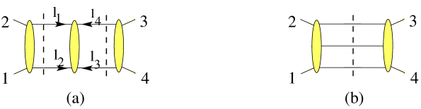
The integrand of the four-point scattering amplitude at two-loops was found in Bern:1997nh and evaluated in Anastasiou:2003kj using the results of smirnov_2loops . It can be evaluated by a considering a double two-particle cut as in figure 7a.
As previously mentioned, they are correctly captured by the rung rule. It is instructive to follow the details of the calculation in this relatively simple case and in the process also have an explicit example of the rung rule; they may in fact be constructed by iteratively using the equation (2.52). For the purpose of the calculation one needs to pick some helicity assignment; we will choose ; thus, we need to evaluate
| (2.60) |
where the helicities of the cut lines are fixed by the requirement that the tree-level amplitudes are nonvanishing. The product of the first two tree-level amplitudes may be easily reorganized following equation (2.52) to be
| (2.61) |
Further application of equation (2.52) leads to a final expression for the product in equation (2.60):
| (2.62) | |||
| (2.63) | |||
| (2.64) | |||
| (2.65) |
where we have used again the cut conditions to organize the result in terms of propagators. One notes without difficulty that momentum conservation implies the cancellation of the numerator factor against the denominator factor in the last equality. This cancellation is crucial for having a Feynman integral interpretation for the generalized cut in equation (2.60). The conclusion of this calculation is that the two-loop four-gluon amplitude contains the double-box integral whose cut appears in the equation above. This calculation also illustrates the application of the rung rule (cf. fig.6).
The other double two-particle cuts are obtained by simple relabeling of the previous calculation. Thus, one finds that they imply that the two-loop four-gluon amplitude in SYM is (for any choice of helicity assignment) given by Bern:1997nh
| (2.66) |
The ultraviolet behavior of SYM suggests121212 Superspace arguments Howe_Stelle_YM imply that at two-loops, SYM is logarithmically-divergent in seven dimensions. This is however only suggestive of (2.66) being the full answer, as there may exist more divergent contributions whose leading ultraviolet behavior cancels out. that this is indeed the complete amplitude, a fact confirmed by the evaluation of the three-particle cut.
Similar (though somewhat lengthier) manipulations or repeated application of the rung rule leads to the three-loop four-gluon amplitude Bern:1997nh , Bern:2005iz . The notable fact is that, unlike the two-loop amplitude, the three-loop integrand retains some dependence of the loop momentum in its numerator.

| (2.68) | |||||
where the integrals are shown in figure 8. The second and third integrals on each row of that figure are equal and also .
A link between lower and higher point amplitudes at any number of loops is provided by the splitting amplitudes introduced in equation (2.20). A unitarity-based all-order proof of those equations as well as a means of directly evaluating the splitting amplitudes was discussed in Kosower_splitting for arbitrary gauge theories. Similar to scattering amplitudes, they are determined by tree-level information up to the appropriate treatment of the intermediate momentum in equation (2.20) which must be kept massive throughout the calculation. The one-loop splitting amplitudes can be obtained without difficulty either by considering collinear limits of higher loop amplitudes Bern_Chalmers or by direct evaluation Kosower_Uwer_1 . The two-loop splitting amplitude in SYM theory have been computed and their properties have been analyzed in QCD_splitting_amplitude , Anastasiou:2003kj .
2.4.1 A possible integral basis at higher loops; Conformal integrals
SYM is a conformal field theory at the quantum level; conformal invariance may be observed in correlation functions of operators of definite (anomalous) dimension. In the context of the AdS/CFT correspondence this symmetry is related to the existence of an exact isometry of the anti-de-Sitter space. At the level of on-shell scattering amplitudes however (super)conformal invariance is obscured beyond tree level; after removing the effects of the (infrared) regulator which explicitly breaks it, the momentum space realization of the generators of the conformal group still exhibits anomalies analogous to the holomorphic anomaly of collinear operators CSWanomaly .
It was observed in Drummond:2006rz by explicitly inspecting the known results for the one-, two- and three-loop four-gluon amplitudes that the integrals appearing in the rescaled amplitude exhibit, if regularized by keeping the external legs off-shell, (in a sense we will describe below) an symmetry apparently unrelated to the four-dimensional conformal group. To expose this symmetry one solves the momentum conservation constraint at each vertex by writing each momentum as a difference of two variables
| (2.69) |
We use the notation here to denote generically both external momenta as well as loop momenta. These variables define the position of the vertices of the dual graph.

This way the momentum conservation constraint is replaced by an invariance under uniform shifts of the dual coordinates . Moreover, their Lorentz transformation properties are identical to those of the momenta. Since the dual variables are unconstrained one may also define an inversion operator
| (2.70) |
An off-shell regularization of infrared divergences allows the construction of planar loop integrals which are invariant under such a transformation. Indeed, properties of dual graphs imply that in any planar integral all inverse propagators can be written as the square of a difference of two -s. Thus, propagators transform homogeneously (with weight in each of the two -s) under the transformation (2.70). The weight of each in the transformation of all propagators defining the integral equals twice the number of propagators containing this variable. The four-dimensional loop integration measure transforms homogeneously (with weight ). It therefore follows that a numerator factor transforming homogeneously with the appropriate weight would render the integral invariant under simultaneous inversion of all dual variables . Simple graphical rules capturing the transformation under inversion of an integral are illustrated in figure 9. Let us illustrate the details by discussing a simple example – the one-loop box integral shown in figure 9a. Up to numerator factors, the relevant integral is
| (2.71) |
each of the propagators present is denoted by a solid line in figure 9a. As mentioned, under inversion this integral transforms as
| (2.72) |
i.e. it transforms homogeneously with weight for each of the coordinates unrelated to the loop momentum. If the external momenta are massless – – then the only way to compensate for this transformation is by adding a factor of since
| (2.73) |
and thus is invariant. If two opposite external legs are massive – say and – a further numerator factor is possible since no longer vanishes and transforms as
| (2.74) |
Further possibilities occur if more of the external legs are massive. A similar discussion may be carried out at higher loops Drummond:2006rz .
One can also define a dilatation generator, under which all integrals transform homogeneously and carry the same weight as under rescaling of momentum variables. Together with translations of the dual variables and their inversion this generate an algebra called dual conformal symmetry.
It turns out that all integrals which appear in the four-gluon amplitude through three-loops are invariant under dual conformal transformations if they are regularized with an off-shell regulator. The amplitudes are however constructed assuming dimensional regularization; due to the change in the dimension of the integration measure this regularization breaks the inversion invariance. Dimensionally-regularized integrals which, if regularized with an off-shell regulator are invariant under dual conformal transformations are called pseudo-conformal integrals DHKS4_2loop . It is interesting to note that by this definition -integrals are also pseudo-conformal. Indeed, with an off-shell regulator the integrand is treated as four-dimensional and thus vanishes identically for these integrals.
The appearance of pseudo-conformal integrals is not limited to four-point amplitudes in SYM; they also generate the scalar factor of -point one-loop MHV amplitudes, the even part of the two-loop five-point amplitude (cf. Figure 9) and the even part of the two-loop six-point amplitude BDKRSVV which we shall review shortly.
It is not clear what is the underlying reason for the appearance of dual conformal invariance at weak coupling. It is moreover not clear whether its appearance persists to all loop orders (perhaps up to integrals whose integrands vanish identically in four dimensions BDKRSVV ). It is nevertheless a useful guide in organizing higher loop calculations. If it indeed survives to all orders in perturbation theory it provides a general (though nevertheless overcomplete at higher loops) basis of integrals organizing parts of higher loop amplitudes in SYM.
2.5 The BDS conjecture and potential departures form it
In section 2.4 we discussed, following Bern:1997nh , Bern:2005iz , higher loop corrections to the four-gluon amplitude. The direct evaluation of the integrals in the two-loop four-gluon amplitude Anastasiou:2003kj reveals a surprising structure: up to terms of order ,
| (2.75) |
Equally surprisingly, the same expression holds for the two-loop splitting amplitude Anastasiou:2003kj . Such an iterative behavior is to be expected for the infrared-singular part of the amplitudes; indeed, it is only a consequence of the soft/collinear factorization theorem discussed previously (cf. eq. (2.42)). The surprising fact is that this structure extends to the finite part of the amplitude, in particular that is a constant.
The fact that splitting amplitudes provide a link between higher and lower-point amplitudes at fixed loop order suggests a generalization of the iteration relation above to arbitrary number of external legs. Indeed, an ansatz which correctly captures the behavior of the amplitude in collinear limits as well as its infrared singularities is
| (2.76) |
Similarly to the explicit calculation of the four-point amplitude, the main feature of this ansatz is that and are independent of the external momenta and also of the number of external legs. The five-gluon amplitude at two-loops obeys this ansatz; the same cannot be said however about the six-gluon amplitude, as we shall discuss in section 2.6.
A similarly surprising result followed Bern:2005iz from the evaluation of the three-gluon amplitude (2.68); throughout the finite part, it obeys an iterative structure similar to that if the two-loop amplitude.
This equation as well as (2.75) are consistent with the resummed amplitude taking an exponential form with the exponent given in terms of the one-loop four-gluon amplitude. Assuming that the same is true for the splitting amplitude, Bern, Dixon and Smirnov Bern:2005iz suggested that, to all loop orders, the rescaled -point MHV amplitude is given by
| (2.77) |
where the coefficients
| (2.78) |
are independent of the number of external legs. The -independent part, , are the Taylor coefficients of the cusp anomalous dimension or universal scaling function (2.38)
| (2.79) |
The appearance of the cusp anomalous dimension is of course dictated by the infrared structure of the amplitude. Similarly, and define the functions
| (2.80) |
the former being twice the first logarithmic integral of entering in the Sudakov form factor (2.39).
In the construction of (2.77) it was assumed that the splitting amplitude obeys an all-order exponentiation similar to the infrared-singular part of the amplitude:
| (2.81) |
This relation may be justified using dual conformal invariance. Indeed, as we will see in some detain in section 4.3.4 following Drummond:2007au , the four- and five-point amplitudes are uniquely fixed by requiring that this symmetry, observed in explicit calculations, exists to all orders in perturbation theory. Then, taking the collinear limit of the five-point amplitude immediately yields (2.81).
The infrared poles are apparent in the equation (2.77) and, using equation (2.42), may be readily isolated together with the associated dependence on the two-particle invariants:
| (2.82) |
where the invariants are assumed to be negative. The functions and are respectively the second and first logarithmic integrals of the functions and . Extracting this divergent part defines the finite remainder .
| (2.83) |
with . In the simplest case of the four-gluon amplitude the finite remainder takes the form
| (2.84) |
For more than four external legs the finite remainders have a more complicated form:
| (2.85) |
where
| (2.86) |
in which is the greatest integer less than or equal to and, as in (2.57), are momentum invariants. (All indices are understood to be .) The form of and depends upon whether is odd or even. For the even case () these quantities are given by
| (2.87) |
In the odd case (), we have,
| (2.88) |
These expressions for and are found BDDK_npt by inserting the explicit values of the box integrals into equation (2.57).
By construction, the BDS conjecture captures the correct infrared singularities as well as the correct behavior under collinear limits. Thus, departures from it should contain no infrared singularities and moreover should have vanishing collinear limits in all channels.
Additional constraints may be found if one assumes that dual conformal invariance is a property of MHV amplitudes to all orders in perturbation theory Drummond:2007au . While it is a plausible assumption especially in light of the strong coupling prescription for the calculation of scattering amplitudes AM1 which we will discuss shortly, this assumption needs to be verified on a case by case basis. Nevertheless, if this assumption holds, it leads to the conclusion that departures from the BDS ansatz must be exhibit dual conformal invariance as a consequence of their finiteness. Thus, similarly to two-dimensional conformal field theories, such corrections must be functions of invariants under the inversion transformations (2.70). Dual conformal invariants can be constructed for any kinematics with at least six momenta. As we will see in more detail in section 4.3.4, in this case they are131313 Parity-odd dual conformal invariants can also be constructed. Explicit calculations CSV_odd_six_pt show that, at least at two-loop order, all parity-odd terms in the six-point amplitude exponentiate following the BDS ansatz.
| (2.89) |
The number of such cross-ratios – i.e. with the difference between any two labels of at least two units – grows with the number of external points. Clearly, dual conformal invariance would imply a reduction in the number of independent arguments of (the finite part of) MHV amplitudes. This point will be further discussed in section 4.3.4.
To probe the structure of amplitudes it is useful to define the remainder function :
| (2.90) |
This is a finite, dual conformally invariant function of the coupling constant which encodes the departure of the -point MHV rescaled amplitude from the BDS ansatz. The part may be readily extracted and reads
| (2.91) |
Note that the terms in parenthesis are just the ABDK ansatz (2.76) for the 2-loop MHV amplitude with arbitrary multiplicity.
2.6 The six-point MHV amplitude at two-loops and the BDS ansatz
As previously mentioned, the ABDK/BDS ansatz was constructed based on explicit calculations of four gluon amplitudes at two- and three-loop orders as well as of the collinear splitting amplitudes at two-loop order and was subsequently tested through the calculation of the five-point amplitude at two-loops. Assuming that dual conformal invariance holds to all loop orders, the fact that no conformal cross-ratios can be constructed for four- and five-point kinematics suggests that these amplitudes are determined to all orders by their infrared singularities. In later sections we will discuss to what extent this interpretation is accurate; the ABDK/BDS ansatz will obey an anomalous Ward identity for dual conformal transformations which has a unique solution for four- and five-point kinematics. Thus, in these cases, the ABDK/BDS ansatz necessarily reproduces the scattering amplitudes.
For higher-point kinematics scattering amplitudes may contain in principle additional information beyond that related to its infrared divergences, which is captured by finite functions of conformal ratios and vanishes in all collinear limits.
Similarly to the five-point MHV amplitude at two-loops, the two-loop six-point MHV amplitude contains an even and an odd part. The even part was evaluated in BDKRSVV and information on the odd part was found in CSV_odd_six_pt . Projecting the ABDK ansatz (2.76) onto parity-even and parity-odd components, it follows quickly that similar iteration relations should hold separately for the even and odd parts of rescaled amplitudes. It turns out that, while the odd part of the amplitude obeys the iteration relation CSV_odd_six_pt , the even part does not, signaling departures from the ABDK/BDS ansatz.
Following the discussion in previous sections, to reconstruct the amplitude one should analyze all of its generalized cuts. The known ultraviolet behavior of the theory however implies certain simplifications. As mentioned before, this is quite analogous to the observation that one-loop amplitudes can be written solely in terms of box integrals. The analogous statement for two-loop amplitudes of arbitrary multiplicity is that they are completely determined by (-dimensional) iterated two-particle cuts. The relevant topologies are listed in figure 10.
Here, as well as for more general amplitudes, it is useful to organize the result as the sum of the part constructible from four-dimensional cuts and the part accessible only through some (partial) -dimensional cuts
| (2.92) |
The latter terms are built from -integrals and their four-dimensional generalized cuts vanish identically (in the sense that all cut propagators are considered four-dimensional).

The four-dimensional cut-constructible parity-even part of the amplitude is given entirely in terms of pseudo-conformal integrals BDKRSVV ;
| (2.95) | |||||
The integrals are listed in figure 11 and the corresponding coefficients for the permutation are:
| (2.96) | |||||
| (2.97) | |||||
| (2.98) | |||||
| (2.99) | |||||
| (2.100) | |||||
| (2.101) | |||||
| (2.102) | |||||
| (2.103) | |||||
| (2.104) | |||||
| (2.105) | |||||
| (2.106) | |||||
| (2.107) | |||||
| (2.108) |
It is not hard to check that all terms appearing in (2.95) are indeed pseudo-conformal integrals. Their relative coefficients are and , which represents a chance of patterns from the four- and five-point amplitudes where they were only and . It is currently unclear what is the origin of this change.
The remaining parity-even part of the amplitude, which may be determined by performing generalized cuts with at least one two-particle -dimensional cut is BDKRSVV
| (2.109) |
the coefficients for the identity permutation are
| (2.110) | |||||
| (2.111) |
Their dual conformal properties are somewhat nontransparent; following the definition given in section 2.4.1 they may be interpreted as pseudo-conformal as their integrand vanishes identically in four dimensions. Explicit calculation BDKRSVV shows that they do not contribute to the remainder function (2.91); thus, their presence may be ascribed to the infrared structure of the amplitude, interpretation strengthened by the fact that they either integrate to () or they exhibit infrared poles ().
The analytic evaluation of the integrals appearing in the six-point amplitude remains a difficult open problem, with potential applications beyond SYM. To test for the structure and the conformal properties of the remainder function, BDKRSVV evaluated the amplitude at a variety of kinematic points through . For the state of the art in the evaluation of Feynman integrals we refer the reader to Smirnov_book , mathematica_implementation1 , mathematica_implementation2 , mathematica_implementation3 . Two of the kinematic points, and , were chosen to have the same cross-ratios while the momentum invariants are different. The results BDKRSVV of the evaluation of the remainder function are shown in table 2.1.
| kinematic point | ||
|---|---|---|
| ( | ||
The main observation is that the remainder function is nonzero to a high level of confidence thus suggesting that the ABDK/BDS ansatz captures only part of the amplitude. It is also important to note that the remainder functions at kinematic points and are equal within within the errors. This strongly suggests that is indeed a function of only conformal cross-ratios – i.e. is invariant under dual conformal transformations.
The conclusion of this calculation is thus that the BDS ansatz should be modified for six point amplitudes and beyond. For this purpose it is instructive to identify the origin of the remainder function within the arguments that led to this ansatz. In short, the full structure of collinear limits for -point amplitudes with is somewhat more involved. One may consider limits in which more than two particles are simultaneously collinear:
| (2.112) |
For the six-point amplitude only a triple-collinear limit (i.e. above) exists. While vanishing in all double-collinear limits, the remainder function for the six-point amplitude has a nontrivial triple-collinear limit, which in fact allows its complete reconstruction. We refer the reader to BDKRSVV for more detailed discussions in this direction.
3 Scattering amplitudes at strong coupling through the AdS/CFT duality
The AdS/CFT correspondence Maldacena:1997re , Gubser:1998bc , Witten:1998qj provides the only direct access to the strong coupling regime of the SYM; it relates four-dimensional SYM theory and type IIB string theory on space through the identification of string states and gauge-invariant operators. The two gauge theory parameters – the ’t Hooft coupling and the rank of the gauge group – are expressed in terms of the radius of curvature of the space and the string coupling by the well-known relations
| (3.1) |
Thus, in the limit of a large number of colors the splitting and joining of strings is suppressed and in the limit of large ’t Hooft coupling, the string theory lives on a weakly curved space. In this regime the string theory is completely described by a weakly-coupled worldsheet sigma-model.
By appending an open string sector to closed string theory in gluon scattering amplitudes could in principle be directly computed, on the string side of the AdS/CFT correspondence, in terms of integrated correlation functions of vertex operators. Due to the presence of color factors it is, however, unclear how much of the resulting structure can be captured entirely in terms of closed string data. We will argue, following AM1 , AM3 , that the color-stripped partial amplitudes do have such a description, to leading order in the strong coupling expansion.
As extensively discussed in the previous section, a further property of on-shell scattering amplitudes is the need of an infrared regulator due to the presence of infrared divergences. Dimensional regularization and variants thereof remain the preferred gauge theory regularization scheme. As we will see, a choice of regularization is also needed to define the scattering on the string theory side of the AdS/CFT correspondence. We will discuss two such choices: first, to set up the calculation, we will use as a regulator a -brane cutting off the infrared part of . After formulating and understanding the prescription for computing scattering amplitudes at strong coupling we will modify the regulator to one akin to the gauge theory dimensional regulator; this will allow a direct comparison with the strong coupling limit of (2.77).
3.1 The general construction
In the presence of an open string sector on the string theory side of the AdS/CFT correspondence, the calculation of open string scattering amplitudes in the Poincaré patch is, in principle, conceptually straightforward: one simply computes the transition amplitude between some in and out asymptotic states. To describe scattering amplitudes of SYM fields, these states must be located at spatial infinity in the directions parallel to the boundary of the space. As usual, two-dimensional conformal invariance on the string worldsheet allows a description of the asymptotic states in terms of local vertex operators inserted on the boundary of the worldsheet.
Perhaps the natural place for the worldsheet boundary and for the vertex operators is the AdS boundary located at in the coordinates141414Notice that we interchanged the notation for original and dual variables with respect to the one used in AM1 .
| (3.2) |
It is however not hard to see that such a choice is not allowed: indeed, scattering amplitudes are expected to be divergent and as such must be evaluated in the presence of a regulator. As discussed at length in section 2, the expected divergences arise from low energy modes; thus, a natural regulator eliminating these modes is a D3-brane placed at some fixed and large value of the radial coordinate and extending along the four boundary directions .
An interesting property of the Poincaré patch is that the spatial infinity of the regulator brane introduced above coincides with the spatial infinity of the AdS boundary.151515It is perhaps interesting to note that, regardless of the coordinate system, a regulator brane excising the part of AdS space describing the low energy modes of SYM theory always intersects the boundary. Consider for example the global coordinates; the global time is dual to SYM energy scale. Eliminating low energy modes amounts to placing a D3-brane at on some surface of fixed time; it is not hard to see that this D3-brane will also intersect the boundary of AdS space. Thus, the asymptotic states of the scattering process are simultaneously defined on the regulator brane as well as on the boundary of space. Two-dimensional conformal invariance may then be used to describe them through vertex operators located either on the boundary or on the regulator brane (see fig. 12).

The momenta carried by vertex operators in these two representations of the asymptotic states are, however, different due to the fact that the anti-de-Sitter space has a nontrivial metric. Indeed, if the vertex operator carried momentum when placed on the boundary, it carries the corresponding proper momentum when placed on the regulator brane
| (3.3) |
Here is the momentum conjugate to the boundary coordinates and must be kept fixed161616 plays the role of gauge theory momentum as the infrared regulator is removed – i.e. . Thus, when described in terms of vertex operators placed on the regulator D3-brane, the scattering process occurs at arbitrarily high (proper) momenta and fixed angle.
In flat space this regime was studied by Gross, Mende and Manes Gross:1987kza , Gross:1989ge . The key result of their analysis is that, to leading order in the large momentum expansion, the calculation of the scattering amplitude is dominated by a saddle point of the classical action, deformed by the insertion of vertex operators. At string tree-level, the worldsheet has the topology of a disk and the vertex operators corresponding to the scattering states are inserted on its boundary. Perturbative corrections to the saddle-point contribution are a series in inverse-momentum invariants (e.g. and for a four-point amplitude) and yield the large energy expansion of the amplitude.
The expansion of scattering amplitudes is thus correlated to the energy expansion; this can be understood on dimensional grounds and it is a feature of the free worldsheet theory for strings in flat space. In curved spaces the situation is different and scattering amplitudes are a double-series in energy and in (inverse) curvature .171717Here denotes the curvature and denotes the curvature radius.
One may repeat the arguments of Gross:1987kza , Gross:1989ge for the gluon scattering amplitude described by vertex operators placed on the regulator brane in AdS space. The fact that the vertex operators are necessarily proportional to and that is large (cf. (3.3)) guarantees that, as the regulator is removed (), the conclusion that the scattering amplitude calculation is dominated by a saddle-point continues to hold, i.e.
| (3.4) |
where is the value of the classical worldsheet action at the saddle-point.181818For sufficiently many particles it is known (in flat space) that there exist multiple saddle-points. The same may happen in AdS space as well. Presumably, for a fixed configuration, a single saddle-point yields the dominant contribution to the amplitude. It would be very interesting to clarify this issue.
As discussed above, this result may receive corrections of two types: corresponding to the large energy expansion and corresponding to the curvature expansion. Corrections of type must then be a series in where denotes some Mandelstam invariant on the regulator brane. Due to (3.3), this is also a series in and thus they are irrelevant as , for any finite, not necessarily large, value of the field theory invariants . Corrections of type are governed by the curvature radius of AdS space. From (3.1) it follows that the curvature expansion is a series in which should therefore reproduce the strong coupling expansion of scattering amplitudes.
To summarize this (long) argument, the leading term in the strong coupling expansion of a scattering amplitude of states in SYM theory is exactly given by the value of the classical worldsheet action at a saddle-point. The corresponding worldsheet has the topology of a disk with boundary placed on the regulator brane and containing the vertex operators describing the scattering states. Corrections around this saddle-point yield the strong coupling expansion of the corresponding amplitude. This analysis captures both the color and the kinematic dependence of amplitudes.
While this conclusion AM1 is very encouraging, the boundary conditions for the construction of the saddle-point cannot be easily formulated due to a lack of sufficiently explicit expressions for open string vertex operators in AdS space. It turns out however that the boundary conditions for the construction of the saddle-point are easier to formulate in terms of the T-dual boundary coordinates. Indeed, consider a metric of the form
| (3.5) |
On an Euclidean worldsheet, the T-dual coordinates are defined by191919This transformation, while identical to T-duality for compact coordinates, should be interpreted here as a formal sigma model duality transformation. Apart from their use here AM1 , such transformations have been also used Kallosh:1998ji to simplify the action of the Green-Schwarz superstring in .
| (3.6) |
For the specific in (3.2) this transformation, combined with the redefinition has no apparent effect on the metric Kallosh:1998ji . Indeed, after the first step the metric becomes
| (3.7) |
which is just another copy of AdS5. The important point however is that, unlike the metric (3.2), its boundary is located at . Further introducing the radial coordinate
| (3.8) |
leads to the metric
| (3.9) |
which is identical to (3.2) except that, as implied by the coordinate transformation (3.8), the boundary of this space should be defined to be at .
The sequence of transformations has important effects on vertex operators and on the regulator brane:
the regulator brane is located at which is located close to the boundary of the resulting space.
T-duality transformation of a compact coordinate interchanges momentum and winding states. The transformation (3.6) has a similar effect: the zero-mode of the field corresponding to the momentum (and described by a local vertex operator) is replaced by a “winding” mode of the field implying that the difference between the two endpoints of the string obeys
| (3.10) |
as may be seen by integrating (3.6) over the space-like worldsheet coordinate (). Thus, each vertex operator is replaced by a line segment connecting two points whose coordinate difference is a multiple of the momentum carried by the vertex operator. Moreover, since the regulator brane is located near the boundary, the momentum carried by these vertex operators is that of the gauge theory scattering states.
To summarize, the boundary conditions defining the saddle-point generating the leading term in the strong coupling expansion of scattering amplitudes (see fig. 13) imply that the boundary of the worldsheet is a line constructed as follows:
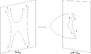
-
•
For each particle of momentum , draw a segment joining two points separated by .
-
•
Concatenate the segments according to the insertions on the disk (corresponding to a particular color ordering or to a particular ordering of vertex operators on the original boundary)
-
•
As gluons are massless, the segments are light-like. Due to momentum conservation, the diagram is closed.
Figure 14 shows an example of such boundary conditions, corresponding to the scattering of six particles.

As the infrared regulator is removed, i.e. as in the original coordinates, the boundary of the worldsheet moves towards the boundary of the T-dual metric, at . To leading order in the strong coupling expansion the computation of scattering amplitudes becomes formally equivalent to that of the expectation value of a Wilson loop given by a sequence of light-like segments.
The standard prescription Rey:1998ik , Maldacena:1998im implies that the leading exponential behavior of the point scattering amplitude is given by the area of the minimal surface that ends on a sequence of light-like segments on the boundary
| (3.11) |
The area contains the relevant kinematic information through its boundary conditions.
It is important to stress the following two points:
In implementing the duality transformation (3.6) at the level of vertex operators most of their structure – in particular the polarization of the particle – was ignored, as we were interested in the leading strong coupling regime. Thus, such information is not directly available at the level of the light-like polygon describing the boundary conditions. To access this information (which may, in some sense, be considered as subleading in the expansion) it appears necessary to return to the vertex operator picture for the scattering process. This should expose, for example, that all-plus helicity amplitudes vanish identically (2.28).
The map (3.10) between vertex operators and light-like segments operates independently of the color structure of the original amplitude. Thus, one finds one light-like polygon for each color-ordered amplitude. The corresponding color factor may be reconstructed from the order of momenta of particles.
In the following, we will show in detail how this construction works for the scattering of four gluons and compare our results with field theory expectations.
3.2 Four gluon scattering
The simplest scattering process involves four particles and is characterized by the usual Mandelstam invariants
| (3.12) |
The discussion in the previous section suggests that, in the strongly coupled SYM theory, the amplitude for this process is governed by the minimal surface ending on the light-like polygon shown in figure 15.

As implied by the equation (3.10), the difference between the coordinates of each of the corners of the polygon (cusps) are, up to a factor of , the momenta of the corresponding gluon. In drawing figure 15, it was assumed that the third component of the momentum (described by the boundary coordinate ) vanishes. This choice imposes no kinematical restrictions, as it does not imply any relations between the two Mandelstam invariants.
The area of a surface embedded in a higher dimensional space is simply given by the integral of the induced metric
| (3.13) |
Finding minimal surfaces amounts simply to treating this area as an action (the Nambu-Goto action) and solving the classical equations of motion, subject to the desired boundary conditions. Then, the area is obtained by evaluating (3.13) on the resulting configuration.
3.2.1 The single cusp solution
As a warm up exercise let us discuss the solution near the cusp where two of the light-like lines meet. This problem was originally considered in Kruczenski:2002fb and it will prove useful for generating the solution relevant for the four-gluon scattering. The surface can be embedded into an subspace of
| (3.14) |
We are interested in finding the surface ending on a light-like Wilson line which is along , 202020One can also consider Wilson loops along . The basic difference with the ones considered here is that their worldsheet is Lorentzian and is imaginary. (see figure 16). This configuration has both boost and scale symmetry, which are made manifest by the following ansatz:

| (3.15) |
This ansatz establishes a close relation between the affine coordinates and the target space coordinates ; boosts in the plane and scale transformations are simply shifts of and , respectively.
Equations for the remaining function may be found by evaluating the equations of motion on the ansatz (3.15). Alternatively, one may simply evaluate the Nambu-Goto action on the ansatz (3.15) and derive an equation for by varying the result with respect to it. Choosing the second path, the Nambu-Goto action becomes
| (3.16) |
One can then explicitly check that solves the equations of motion and has the correct boundary conditions. Hence the surface is given by
| (3.17) |
Notice that the surface lies entirely outside the light-cone of the origin, hence it is Euclidean.
3.2.2 Four cusps solution
The four cusps solution is closely related to the single cusp solution discussed above. The relevant solution of the Nambu Goto action can be embedded in a subspace of , parametrized by . It is moreover convenient to fix reparametrization invariance by choosing . With these choices, the Nambu-Goto action describes the dynamics of two fields, and , living in the space parametrized by and
| (3.18) |
The classical equations of motion should then be supplemented by the appropriate boundary conditions. We consider first the case with , where the projection of the Wilson lines is a square. By scale invariance, we can choose the edges of the square to be at . The boundary conditions can be easily seen to be
| (3.19) |
The form of the solution near each of the cusps can be obtained by rotations and boosts from the single cusp solution (3.17). The following field configuration satisfies the boundary conditions and has the correct properties near each of the cusps
| (3.20) |
Remarkably it turns out to be a solution of the equations of motion. However, in order to capture the kinematical dependence of the area 212121On dimensional grounds the area, if finite, should be a function of the form . we need to consider more general solutions with . In this case the projection of the surface to the plane will not be an square but a rhombus, with and given by the square of the distance between opposite vertices, as shown in figure 17.

The symmetry generators of anti-de-Sitter space act nonlinearly on the Poincaré patch coordinates (3.9). They are however useful for generating new and interesting worldsheet configurations from known ones, since they can change the Mandelstam variables and ; it would therefore be useful to linearize their action. This is realized by passing to the so-called embedding coordinates, in which is viewed as a hypersurface
| (3.21) |
embedded in . Clearly, this constraint equation is manifestly invariant under the symmetry group of , which is also the Lorentz group of the embedding space. The Poincaré coordinates are but a particular solution of the constraint equation (3.21):
| (3.22) | |||||
Direct use of the solution (3.20) implies that, in the embedding coordinates, the minimal surface describing the scattering of four gluons with the kinematics is
| (3.23) |
In this form it is then easy to use the to generate from (3.20) new minimal surfaces, corresponding to gauge theory kinematics.
Through the AdS/CFT correspondence, the of the dual AdS space should have a gauge theory counterpart. Due to the T-duality transformation relating the boundary coordinates of this space with gauge theory momenta this symmetry is necessarily different from the usual position space conformal invariance of SYM theory. As discussed in section 2.4.1, the action of a “dual conformal group” can be identified at the level of perturbative scattering amplitudes. While a priori these two symmetries are unrelated (as e.g. the former exists at strong coupling while the latter at weak coupling), it is nevertheless tempting to interpret the latter as the weak coupling version of the former. This interpretation is strengthened by the relation between MHV scattering amplitudes and Wilson loops, which will be discussed in section 4.
Solutions with can be obtained by starting from (3.20) and performing a boost in the plane. In this way we change the distance between opposite vertices of the square.
| (3.24) |
After the boost, we end up with a two-parameter solution, one related to the size of the initial square and another related to the boost parameter. The solution can be conveniently written as
| (3.25) | |||
| (3.26) |
where we have written the surface as a solution to the equations of motion in conformal gauge
| (3.27) |
and encode the kinematical information of the scattering as follows
| (3.28) |
To obtain the four point scattering amplitude at strong coupling it should suffice, following the discussion in section 3.1, to evaluate the classical action on the solution (3.25). However, in doing so, one finds a divergent answer. That is of course the case, since we have ignored the infrared regulator. In order to obtain a finite answer we need to reintroduce a regulator.
3.2.3 Dimensional regularization at strong coupling
Gauge theory amplitudes are regularized by considering the theory in dimensions. More precisely (see discussion in section 2), one starts with in ten dimensions and then dimensionally reduces to dimensions. For integer this is precisely the low energy theory living on a brane, where . We regularize the amplitudes at strong coupling by considering the gravity dual of these theories. 222222See section 3.5 for a brief discussion of the subtleties of sigma-model actions in these backgrounds and the calculations of corrections to the classical area of the minimal surface. The string frame metric is (see e.g. Duff:1994an , Itzhaki:1998dd )
| (3.29) |
Following the steps described above, one is led to the following action
| (3.30) |
Where is the Lagrangian density in the absence of the regulator. The presence of the factor , which arises from the conformal factor of the induced metric, will have two important effects. On one hand, previously divergent integrals will now converge. On the other hand, the equations of motion will now depend on and it turns out to be very difficult to find the solution for general . However, we are interested in computing the amplitude only up to finite terms as we take . In that case, it turns out to be sufficient to plug the original solution into the -deformed action 232323Up to a contribution from the regions close to the cusps that add an unimportant additional constant term.. The evaluation of integrals leads to AM1
| (3.31) |
Finally, expanding in powers of yields the final answer
| (3.32) | |||||
| (3.33) | |||||
| (3.34) |
This should be compared with the field theory expectations, equations (2.82) and (2.83), specialized to the case :
| (3.35) | |||||
| (3.36) |
It is important to notice that the general structure is in perfect agreement with the general structure of infrared divergences in SYM theory. It is not hard to see that the leading divergence has the correct coefficient, given by the strong coupling limit of the cusp anomalous dimension Kruczenski:2002fb 242424The appearance of the cusp anomalous dimension in the equations (3.35) may appear surprising at first sight. Indeed, by analogy with weak coupling arguments based on finiteness of physical quantities constructed from gluon scattering amplitudes, the natural quantity entering (3.35) should be the large spin limit of the anomalous dimension of twist-2 operators. It was however shown in Kruczenski:2007cy that worldsheet calculations of the cusp anomaly and of the large spin limit of the anomalous dimension of twist-2 operators are related by an analytic continuation and and target space symmetry transformations. Thus, similarly to the weak coupling result of cusp_vs_twist2_1 , cusp_vs_twist2_2 , Bassetto:1993xd , the cusp anomaly equals the large spin limit of the anomalous dimension of twist-2 operators to all orders in the expansion.
| (3.37) |
Moreover, from (3.32) one could extract the strong coupling behavior of the function introduced in equation (2.80):
| (3.38) |
Notice that due to the scheme dependence of , it should be computed using the same regularization as in perturbative computations, that of course is not the case for . Finally, the kinematic dependence of the finite term (3.35) reproduces the strong coupling limit of the BDS prediction (2.83)-(2.84) for the four gluon scattering amplitude.
3.2.4 Radial Cut-off
A more common regularization scheme for computing minimal areas in is to introduce a cut-off in the radial direction. The correct procedure would be to impose the boundary conditions at some small . It turns out, however, that in order to compute the finite piece as it suffices to use the original solution and cut the integral giving the area at 252525This finite part arises in a similar way when using the conjectured string theory version of gauge theory dimensional regularization.
In order to compute the regularized area for the scattering of four gluons it is convenient to work in conformal gauge. In this case, the problem reduces to the calculation of the area enclosed by the curve
| (3.39) |
One way to compute the area is by expanding the integrand in power series of and integrating term by term. Equivalently, one can use Green’s theorem and express the area as a one dimensional integral over the boundary of the worldsheet. The result is
| (3.40) |
Several comments are in order. First, notice that the structure of infrared divergences is of the form 262626Notice that a very similar structure appears when using off-shell regularization, as done in Drummond:2007aua ., and the coefficient in front of double logs and the finite piece is proportional to the cusp anomalous dimension at leading strong coupling, as in the case of dimensional regularization. Second, single logs have been absorbed into the double logs. Finally, the finite term reproduces, up to an additive constant, the results of dimensional regularization. Hence, the computation of amplitudes at strong coupling does not need to be done by using dimensional regularization, unless we are interested in computing the function and the constant entering in equations (2.82) and (2.83), respectively, and computed by using dimensional regularization.
3.2.5 Structure of infrared poles at strong coupling
Even if the relevant solutions for minimal surfaces for the cases are presently unknown, the IR structure of amplitudes at strong coupling for the general case of point amplitudes can easily be understood.
Given the cusp formed by a pair of neighboring gluons with momenta and we associate the kinematical invariant . We expect the following structure for the infrared-divergent part of the action
| (3.41) |
where can be computed following Buchbinder:2007hm , either by using dimensional regularization or a radial cut-off. For later applications the later scheme will be more useful to us, in this case
| (3.42) |
Hence, when using a radial cut-off as regulator, we expect the following structure for scattering amplitudes at strong coupling
| (3.43) |
It is easy to check that the general form of the amplitude for the case is consistent with this general expression.
For the discussion of the next subsection, it will be important to consider a radial cut-off that depends on the point at the boundary we are approaching, i.e. . In that case, the structure of the amplitude turns out to be as follows
| (3.44) |
The last sum in this expression corresponds to finite extra contributions coming from the edges
| (3.45) |
where running from zero to one parametrizes the edge, namely and is a shorthand notation for . For instance, a simple example is that of a cut-off that takes the value at the cusp and varies linearly between cusp and cusp, in this case
| (3.46) |
3.3 A conformal Ward Identity
An important ingredient in the construction of the minimal surface governing the four-gluon scattering amplitude was the existence of a dual symmetry.272727In principle this symmetry is unrelated to the original conformal symmetry. It has been suggested RTW that, at the level of the worldsheet sigma-model, the symmetries of the dual space are in fact part of the hidden (non-local) symmetries of the original space sigma-model BPR . This symmetry allowed the construction of new solutions and fixed the finite piece of the scattering amplitude. Naively, this conformal symmetry would imply that the amplitude is independent of and , since they can be sent to arbitrary values by a dual conformal symmetry. The whole dependence on and arises due to the necessity of introducing an infrared regulator. However, we will see that, after keeping track of the dependence on the infrared regulator, the amplitude is still determined by the dual conformal symmetry.
At quantum level, classical symmetries manifest themselves through the existence of (potentially anomalous) Ward identities, the simplest is the quantum version of the conservation of the Noether current. More complicated Ward identities describe the action of symmetry generators on gauge-invariant quantities and potentially constrain their quantum expressions. In this direction it is possible to construct Ward identities for the dual symmetry and study the constraints they impose on scattering amplitudes. For this purpose it is convenient to regularize the amplitude calculation with a radial cut-off.
Given the momenta of the external gluons, the boundary of the worldsheet contains cusps located at , with . Now imagine that we regularize the area by choosing a cut-off . Moreover, we would like this cut-off to depend on the point at the boundary we are approaching, i.e. . From the discussion above we expect the regulated area to have the general form
| (3.47) |
where we have ignored extra terms coming from the edges of the contour as they can be seen not to affect the following argument 282828One can convince oneself, for instance, by considering the simplified case (3.46) and applying the generator of special conformal transformations to such extra terms. It is also instructive to apply the generator of dual conformal transformations, whose relevant piece is of the form , to the general extra terms (3.45) and compare this expression to eq. (34) of Drummond:2007au .. transformations will then act on the points and . By requiring the area to be invariant under the action of special conformal transformations generated by
| (3.48) |
one may derive an equation for the finite part of the amplitude. 292929As the introduction of a infrared cut-off breaks (dual) conformal invariance, one obtains terms that depend explicitly on on the right hand side of (3.48). As we take , conformal invariant is recovered and such terms vanish. At weak coupling this equation was constructed in Drummond:2007au from the analysis of the dual conformal properties of Wilson loops in dimensional regularization. Its strong coupling counterpart was constructed inKomargodski:2008wa using the strong coupling version of dimensional regularization discussed in section 3.2.3.
Assuming that dual conformal symmetry is present beyond the strong coupling limit, a similar argument can be extended to all values of the coupling, e.g. by using as regulator an energy scale and assuming that the amplitude has divergences which depend only on at the cusps (or assuming that special conformal transformations annihilate the extra pieces coming from the edges, as happened at strong coupling.) In the next section it will be discussed how the same Ward identity arises when studying the conformal properties of cusped light-like Wilson loops.
It turns out, that for the case of and , this equation fixes uniquely the form of the finite piece, to be the one in the BDS conjecture. At this point we do not know if the dual conformal symmetry is an exact property of planar amplitudes. We do know, however, that it is a symmetry of all the weak and strong coupling computations that have been done so far. If we assume that it is a symmetry, then we conclude that the BDS conjecture for four and five gluons is correct.
3.4 Other processes
3.4.1 Processes involving asymptotic gluons and local operators
It is natural to extend the discussion in section 3.1 to cover the decay of fields which couple to the SYM fields through some gauge-invariant operators 303030Such couplings are toy models for effective interactions arising from integrating out heavy fields.
| (3.49) |
While these fields may be dynamical, we will not be interested in their other interactions focusing only on processes containing a single field .313131This guarantees that the deformation (3.49) can be treated at the linearized level and thus it does not lead to any modifications to the geometry. We have in mind processes similar to the ones that arise when we consider jets 323232Other interesting processes are the electron-quark elastic scattering or the Higgs boson decaying into two gluons, the later described by the Sudakov form factor.. In this case, we can analyze the process to lowest order in the electro-magnetic coupling constant but to all orders in the strong coupling constant (taken here to be the ’t Hooft coupling) by noticing that the photon couples to the electromagnetic current of QCD and this in turn can produce various final states. Thus the final hadronic state is produced by acting with the QCD electromagnetic current on the vacuum. To lowest order in the state is, of course, a quark-antiquark pair.
We now want to consider analogous processes in super Yang Mills at strong coupling in the planar approximation. Thus we consider a process where we add a local operator to the theory and we produce gluons. The local operator is a single trace operator with given momentum
| (3.50) |
We can consider any operator of the theory. Concrete examples are the stress tensor, the R-symmetry currents, etc.
We are interested in exclusive final states consisting of individual gluons, or other members of the supermultiplet. From now on the word “gluon” will mean any element of the supermultiplet: a gluon, fermion or scalar, all in the adjoint representation. The asymptotic states for these colored objects are well defined only in the presence of an infrared regulator. The simplest one is dimensional regularization, which consists in going to dimensions. Then the theory is free in the infrared (2.40) and gluons are good asymptotic states. On the gravity side this can be done by considering the near horizon metrics of D- branes with , as explained in sec. 3.2.3.
Once we regularize, we have a worldsheet whose boundary conditions in the far past or future are set at , where the asymptotic gluons live, and the operator conditions are set at the boundary of , , in (3.2) . In the T-dual coordinates the asymptotic states carry winding number which is proportional to the momentum. The gluon final states are represented as before by considering a sequence of light-like lines at . Each light-like segment joints two points separated by . As opposed to the situation considered in 3.1, this sequence is not closed. In fact we have where is the momentum of the operator. It is convenient to formally think of the coordinate along as compact and to consider a closed string as winding that coordinate. This is equivalent to saying that we consider an infinite periodic superposition of the set of momenta .
We now should give a prescription for the operator. An operator insertion leads to a string that goes to the boundary, in the coordinates (3.2). This implies that it should go to in the dual coordinates. Thus we consider a string stretching along the direction that goes to .
As a simple example, consider a two gluon state and an operator insertion. The two gluon momenta obey . Let us consider the case where the momentum is spacelike and is incoming and outgoing. By performing a boost we can choose the momenta as
| (3.51) |
It is convenient to view the direction as a compact direction with period so that the total winding number of the string corresponds to an allowed closed string. This closed string has to end on the boundary of the original space (3.2) at . In terms of the dual metric (3.9) it should go to .

In order to find the surface it is convenient to consider an infinite repetition of these momenta, which are following a zig-zag path in the plane as shown in figure (18).
We look for a worldsheet which is extended in the radial direction, from , where it ends on the contour displayed in picture (b), and extends all the way to . As we go to large the surface is extended in the spatial direction but is localized in time. See figure (19) for a picture of the expected surface.
The amplitude is given by computing the area over one period of the resulting surface, since this is the region of the worldsheet that corresponds to the scattering process. Let us point out some features of the solution, which we have not found explicitly. First, one can write the Nambu-Goto action by choosing and as worldsheet coordinates so that is the unknown function. The action is
| (3.52) |
The equations of motion coming from this action should be supplemented with the appropriate boundary conditions
| (3.53) |
and extended in a periodic way outside this range, . This equation could, in principle, be solved numerically. We expect that for distances much bigger than the size of the zig-zag, i.e. , is very small and satisfies a linear equation obtained by expanding (3.52) for small . Expanding in Fourier modes, , with , we obtain the following equation for
| (3.54) |
where we have kept only the decaying solution (for positive ). Note that due to the exponential decay, already when is a few times bigger than , the above solution will be a good approximation. The coefficients are determined by imposing the boundary condition at (3.53) , but we should recall that we cannot use the linearized equation in that region.
The problem has a scaling symmetry that implies that we can scale out so that the solution is
| (3.55) |
It is then easy to see, that the value of the classical action (3.52) on this solution is formally independent of the scale , as expected from scaling symmetry. However, since there is a divergence, an explicit dependence is introduced when we subtract the divergence. Let us understand the divergences. Let us first consider the large region. The integral in the region of large converges since so that we are simply integrating . This might seem a bit surprising since we expected to obtain terms of the form that are related to the anomalous dimension of the operator. Notice, however, that a logarithmic term in the classical area would have implied an anomalous dimension of order . Thus, the boundary conditions we considered correspond to operators whose anomalous dimension vanishes at this order. For a protected operator such as the stress tensor, whose dimension equal to four, this is indeed the case. We expect to obtain logarithmic terms when we go to higher order in the expansion.
We can now consider the small region. The analysis of this region is the same as the analysis in the small region for the gluon scattering amplitudes discussed at the beginning of this section. One can dimensionally regularize the problem by going to dimensions. Then the Lagrangian becomes
| (3.56) |
where we have rescaled all variables so that the only dependence on is in the overall factor. In (3.56) is a function of only . The divergences arise from the region near the cusps connecting the momenta of two adjacent gluons and they can be computed using the single cusp solution considered in section 3.2.1. The value of the action is given by integrating only over one period in . It evaluates to a function of the form
| (3.57) |
The coefficients of the divergent terms are locally determined and are the same as in 3.2.3, so that we would only need the solution to compute the constant . For the simplest case of two gluons, the solution does not depend on any kinematical variable. As we consider configurations with more gluons the solution, and the value of the amplitude, will start depending on the kinematic invariants.
3.4.2 Processes involving a mesonic operator and final quark and antiquarks
In this subsection we consider a small variant of the configuration considered above. We consider a large theory with flavors and we insert a mesonic operator, which contains a quark and an antiquark field.333333Here and elsewhere quarks denote fields in the fundamental representation of the gauge group. For their color charge if which, in the planar limit, is half of the charge of an adjoint field . Flavors correspond to adding D-branes in the bulk Aharony:1998xz , Karch:2002sh , Kruczenski:2003be . A mesonic operator corresponds to an open string mode on the D-brane that is extended over . For example, we could consider the insertion of a flavor symmetry current which couples to a pair. This is analogous to the electromagnetic current in QCD. Other amplitudes involving quarks have been considered at strong coupling in Komargodski:2007er , McGreevy:2007kt and will be reviewed in the next subsection.
In the presence of the infrared regulator, the quarks correspond to open strings that are attached to the D-brane and sit at or . The discussion is very similar to the one for closed strings. One difference is that now we do not require the configuration to be periodic. However, since we obey Neumann boundary conditions on the boundary of the open string, which translate to Dirichlet boundary conditions in the T-dual variables, we find that the solution can be extended outside the strip into a periodic function with a period which is twice the original width of the strip, see figure (20) .

Thus, if we consider a configuration with momenta as in (3.51), the solution is simply given by
| (3.58) |
where is the rescaled solution with period one. The action is simply half of the action (3.57) but with the replacement . After we re-express it in terms of we obtain
| (3.59) |
Thus we see that function which determines the subleading infrared divergences is different for a gluon than a quark. Namely, we have
| (3.60) |
where was computed in the previous subsection. Due to the collinear nature of the function , in the case that we have a cusp that joins a quark and a gluon we expect to have the average of the above two formulas 343434In another words, should measure the contribution coming from the region closed to the edges joined by the cusp.. Similarly, we can consider asymptotic states corresponding to a quark and a antiquark plus extra gluons.
3.4.3 Processes involving quarks and gluons
Scattering of quarks and gluons were considered in Komargodski:2007er and McGreevy:2007kt . As already mentioned, we can have fundamental matter by adding extra D-branes in the bulk. More precisely, we add D7-branes that wrap an in the . Such configuration preserves SUSY. As long as the back reaction of the D7-branes can be ignored and they may be treated as probes.
The quarks will then be given by open strings between the infrared regulator D3-brane and the D7-branes. 353535This is consistent with the fact that quarks transform in the fundamental representation of , while gluons transform in the adjoint representation. Scattering amplitudes can then be computed by considering a worldsheet with the topology of a disk with vertex operator insertions, corresponding to open strings states belonging either to the or sector; the former are gluons and the latter are quarks. For instance, in figure 21 we can see amplitudes corresponding to the scattering of quarks and gluons (a) and only quarks (b).
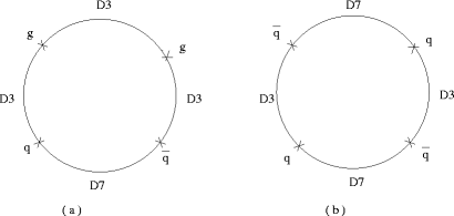
As before, it is convenient to T-dualize along the directions longitudinal to the regulator D3-brane. Such directions are also shared by the D7-branes, so the coordinates satisfy Neumann boundary conditions on the boundary. Hence, after performing the T-duality, the projection of the worldsheet to the boundary of is again a polygon formed by light-like edges given by the momenta of the particles undergoing the scattering. A crucial difference, however, is the following: the components of the boundary ending on the regulator D3-brane have Dirichlet boundary conditions on the radial direction . When the boundary ends on the D7-branes, on the other hand, it satisfies Neumann boundary conditions on the radial direction, so it can extend into the bulk. This implies, that after T-duality, at the location of a cusp between two quarks (or quark-antiquark), the worldsheet can extend into the bulk, folding back into itself, see figure 22 363636We thank the authors of McGreevy:2007kt for providing us with this figure..
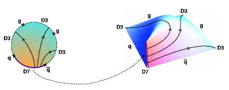
In McGreevy:2007kt it was shown that amplitudes for quarks and gluons at strong coupling can be constructed from special gluon amplitudes. For instance, based on symmetry arguments, the authors have argued that the minimal surface for the amplitude with momenta and , is half of the surface corresponding to the scattering of six gluons with momenta and . 373737More precisely, it can be seen that the polygon corresponding to the scattering of six gluons crosses itself at the midpoints of the lines associated with and , which we can fix at . Then, the worldsheet maps into itself under , where denotes reflection through the intersection point and is the worldsheet parity. The part of the worldsheet at is invariant under such transformation and it can be shown that the radial coordinate satisfies Neumann boundary conditions there. Using the known expression for the divergent piece of such amplitude one obtains
| (3.61) |
As the finite piece of the six gluons amplitude is at present unknown, only the divergent part of the above amplitude can be computed. By looking at the relevant diagrams in the double line notation, McGreevy:2007kt argued that the exchange of soft gluons between quark and antiquark in the above configuration is suppressed by a factor , and so it vanish in the large limit. As a result it is appropriate to rewrite the amplitude (3.61) in the following way
| (3.62) |
with the collinear anomalous dimension between two gluons and the one between a gluon and a quark. Using the known strong coupling expressions for the collinear anomalous dimension for gluons and the cusp anomalous dimension we obtain
| (3.63) |
This result realizes the expectation, discussed in the previous section, that the collinear anomalous dimension for a pair quark-gluon is the average of the collinear anomalous dimension for two gluons and the one for two quarks.
3.5 Further generalizations
In the following we briefly describe many generalizations of the results presented in this section. We refer the reader to the original literature for the details.
According to the discussion in section 3.1, the calculation of the scattering amplitudes in SYM theory at strong coupling is equivalent to finding the regularized area of a minimal surface ending on a special polygon with light-like edges on the boundary of anti-de-Sitter space. While it may be possible to find their areas without actually knowing the solution for minimal surfaces, the most direct approach requires first constructing the classical solutions to the worldsheet equations of motion and then evaluating their areas using perhaps one of the regulators discussed in previous sections. Explicit results for the strong coupling limit of scattering amplitudes may shed light on the resummation of such amplitudes for general number of external legs.
In section 3.2.2 we have described the solution corresponding to the case of four light-like edges. Once a solution is found, additional ones may be constructed through transformations.383838Such solutions were explicitly constructed in Ryang:2007bc . It should be mentioned that, while is a symmetry of the action in the absence of the regulator, it is no longer so once a regulator is introduced. The value of the regularized area will depend on whether the regulator is introduced before or after the transformation is performed. The construction of minimal surfaces ending on polygons with more sides, however, appear to be a much harder problem. Partial progress towards such a goal has appeared in the literature:
-
•
The authors of Jevicki:2007pk , Jevicki:2007aa showed how to apply the dressing method in order to construct new classical solutions for Euclidean worldsheets in . While these solutions may be useful in order to study certain Wilson loops by means of the AdS/CFT duality, their boundary conditions do not correspond to the boundary conditions relevant for studying scattering amplitudes.
-
•
Some partial progress in constructing approximate solutions with light-like polygonal boundary conditions was presented in Itoyama:2007ue , Itoyama:2007fs , Itoyama:2008je . Assuming the BDS ansatz holds and making use of the demonstrated equivalence of one-loop MHV amplitudes and light-like Wilson loops Drummond:2007aua , BHT which will be discussed in detail in section 4, the prescription for computing scattering amplitudes at strong coupling can be written in purely geometrical terms, of the schematic form
(3.64) Here is a function solely of the coupling constant, is a light-like polygon, the left hand side of the above equation is, up to a factor of , the one loop MHV amplitude associated to and is the area of the minimal surface ending on . Conversely, departures from the above relation imply departures from the BDS ansatz at strong coupling. Such departures can be studied for some particular examples by considering approximate solutions. While such approach seems interesting, unfortunately it has not lead to new solutions yet.
-
•
Solutions corresponding to the scattering of six and eight gluons were discussed in Astefanesei:2007bk . In particular, the authors construct new solutions by cutting and gluing the known solutions. However, these solutions appear to satisfy extra boundary conditions and are not clearly related to the relevant solutions.
-
•
In Dobashi:2008ia , a method was developed in order to construct numerically new solutions relevant to scattering amplitudes. The method consists in solving the discretized equations of motion with a given boundary condition. A difficulty in the numerical evaluation of the area, is the need of a regulator. This causes large errors in the computation of the finite piece of the area. However, given the difficulties in constructing analytical solutions, a numerical approach may be appropriate. Besides, the study of numerical solutions can give a hint about their analytical properties.
The part of the bulk geometry as well as the fermionic sector of the theory did not play any role in the strong coupling arguments relating scattering amplitudes and cusped light-like Wilson loops described in section 3.1. This suggests, at least in the strong coupling limit, a certain degree of universality of the results, extending beyond the planar SYM theory. The string theory analysis was carried out for several other theories, for some of which the analog of the BDS ansatz is also available.
-
•
In Nastase_finite_T the prescription was extended to the case of SYM at finite temperature. In this case, the gravity dual is described by the black hole metric, of the form
(3.65) with the temperature . After T-dualizing and performing the change of coordinates , we are led to the action
(3.66) The authors define gluon scattering amplitude at strong coupling and finite temperature by a light-like Wilson loop living at the horizon of this dual metric. Unlike the zero temperature case, now the -dual metric is different from the original metric. As a consequence, this is best interpreted as a way of evaluating scattering amplitudes at finite temperature rather than as a duality between amplitudes and Wilson loops. Quite interestingly, both scattering amplitudes and Wilson loops in the original geometry are related to observables of the theory: the usual Wilson loop to the jet quenching parameter and the scattering amplitude to the viscosity coefficient.
-
•
In OzTY scattering amplitudes in planar -deformed SYM were considered.393939The -deformation is an exactly marginal deformation of SYM theory. The supersymmetric version, due to Leigh and Strassler LeighStrassler , amounts to adding a completely symmetric term in the superpotential. An alternative presentation of the theory is a noncommutative deformation of SYM in which the noncommutative product is based on the R-charge of fields – where is the charge vector of the field and is a real antisymmetric matrix. This formulation allows for simple non-supersymmetric generalizations frolov_beta . The gravity dual of the theory was constructed in Lunin_Maldacena while that of the nonsupersymmetric deformations in frolov_beta . In particular, the authors have considered deformations that break supersymmetry down to and . It was known Khoze_beta that, for real deformation parameter , that planar scattering amplitudes in these theories are the same as in SYM, order by order in perturbation theory. In OzTY it was found that the same conclusion holds in the strong coupling expansion. This is no longer true for complex deformation parameters; starting at five-loop order, the scattering amplitudes in the deformed theory are different Khoze_beta from those of SYM.
The planar scattering amplitudes of orbifolds of SYM theory are also known BerJoh to be identical to those of the parent theory, up to a trivial rescaling of the coupling constant. The strong coupling expansion enjoys similar properties.
-
•
Finally, theories with matter in the fundamental representation were considered by Komargodski:2007er , McGreevy:2007kt and were discussed in some detail in the previous subsection.
A further question, discussed in some detail in Kruczenski:2007cy , is whether the agreement between the BDS ansatz and the result of the AdS/CFT calculation for the four-gluon scattering amplitudes extends beyond the leading order in the strong coupling expansion. To this end it is necessary to evaluate the quantum corrections to the regularized area of the minimal surface, i.e. the corrections to the worldsheet partition function in the presence of the minimal surface background. The strategy is clear and has been extensively applied to the calculation of the energy of extended string solutions: one simply expands the relevant worldsheet action Kallosh:1998ji around the minimal surface and integrates out the fluctuations. For example, the leading correction is given by the logarithm of the ratio of determinants of the bosonic and fermionic fluctuations. This analysis was carried out Kruczenski:2007cy , with some negative conclusions: (a) it is not clear how to construct the complete worldsheet action for D branes; (b) perturbative inclusion of the regulator both at the level of the worldsheet action as well as in the minimal surface leads to a divergent answer at one-loop level. Indeed, since the worldsheet theory is conformal (in a two-dimensional sense), the nontrivial conformal factor in the induced worldsheet metric, which is the basis of the regularization discussed in section 3.2.3, drops out of the calculation of one-loop corrections. Thus, it appears to be necessary to either have an exact minimal surface in the regularized geometry or to switch to a different regulator. The evaluation of corrections to the area of the minimal surface describing the scattering of four gluons at string coupling remains an interesting open question.
4 Scattering Amplitudes vs. Wilson loops at weak coupling
The discussion in the previous section connects (to leading order in the strong coupling expansion) two apparently different quantities: scattering amplitudes and the expectation value of a special type of Wilson loops. Without additional specifications this relation is restricted to MHV amplitudes which, as discussed in section 2, are completely defined by a single function . To be specific, an MHV amplitude is conjectured to be equal to the expectation value of a Wilson loop constructed from noncollinear light-like segments connecting points defined by , as in the equation (3.10).404040The apparent factor of difference between and equation (3.10) may be explained away by invoking the invariance of the expectation value of the Wilson loop under scale transformations.
4.1 The general statement
While the arguments discussed in the previous section are phrased in the string theory dual to SYM theory, the final statement appears to be independent of the coupling constant. Despite the fact that neither scattering amplitudes nor this particular type of Wilson loops are BPS quantities, one may conjecture Drummond:2007aua , BHT a weak coupling relation of a similar type as at strong coupling:
| (4.1) |
Here is the -loop correction to the rescaled MHV amplitude (2.30) and is the -loop correction to the expectation value of the corresponding Wilson loop. As usual, given a contour , a Wilson loop is defined as
| (4.2) | |||||
| (4.3) |
where , are the generators in the fundamental representation and is the dimensionally regularized SYM action. For “standard” Wilson loops is a closed contour in position space, parametrized by an affine parameter : . In the present case, however, is a curve in a configuration space defined such that the difference of the coordinates of two points is a momentum; it is in fact the same Wilson loop described at strong coupling. The SYM is defined on the same space. In this section we will review this remarkable conjecture and the evidence for it.
For SYM theory one may identify the space with coordinates with the position space the theory is originally defined on. Expectation values of light-like Wilson loops defined on this space are then translated to momentum space through the identifications with labeling the cusps of the Wilson loop. Such identifications are specific to conformal field theories and are related to the fact that the position and momentum space can be trivially mapped into each other. The strong coupling arguments described in section 3 imply however a more general relation – that scattering amplitudes of a gauge theory with a string theory dual can be evaluated as expectation values of Wilson loops in the dual momentum space regardless of whether the relevant T-duality transformation leaves the boundary geometry invariant. For this reason we will interpret in the following the Wilson loops as defined directly in the configuration space with coordinates related to particle momenta by . The corresponding conformal group is that acting in momentum space, i.e. the dual conformal group.
It was mentioned briefly in section 2 that higher-loop and higher-multiplicity rescaled MHV amplitudes possess a parity-odd component, proportional to the Levi-Civita tensor. Such components cannot appear in a Wilson loop calculation. In all available explicit calculation the parity-odd part of MHV amplitudes exponentiates (following the BDS ansatz) and this drops out of the left hand side of equation (4.1). This is consistent with the right hand side of that equation being expressible in terms of the expectation value of a Wilson loop. It thus follows that the equation (4.1) suggests that a odd remainder function does not exist to any loop order.
Before proceeding it is worth mentioning that (4.3) is the standard definition of a Wilson loop in a generic YM theory. In SYM this definition is usually modified to include scalar fields; for a generic curve describing also some contour on this is
| (4.4) |
The condition that this Wilson loop is a protected operator is that
| (4.5) |
As described in section 3, has no component on , so . Nevertheless, since it is constructed out of light-like segments, and thus this loop is (locally) BPS away from the cusp. It however enjoys little or no protection from supersymmetry; since the supersymmetry generators preserved by each segment are different, the complete loop is not supersymmetric.
4.2 The MHV amplitudes – Wilson loop relation at one-loop
The perturbative evaluation of the expectation value of the Wilson loops (4.3) (and, generally, of any Wilson loop) is quite straightforward: one expands the exponent while keeping track of the path ordering and then one evaluates the expectation value in equation (4.3) by Wick-contracting the resulting fields either among themselves or with fields from the Lagrangian. The gluon two-point function on this configuration space parametrized by is constructed in the standard way, by transforming from the Fourier conjugate space. In Feynman gauge the result reads414141It is important to keep in mind that, similarly to Feynman diagram calculations of scattering amplitudes, different gauges lead to different forms for the two-point function and thus to different expressions for each contribution to the expectation value of the Wilson loop and some gauges may be more useful than others for exposing specific properties of the final result.
| (4.6) |
The dimensional regulator with appears due to the regularization of the action (and thus of the Fourier transform) and is necessary because the cusps introduce divergences. If this were a “standard” Wilson loop in Minkowski space the divergences appearing due to the presence of cusps would be due to short distance effects. Thus, the regulator is labeled as “ultraviolet” Drummond:2007aua . In the present context, the divergences are due to low energy and to low transverse momenta, so the divergences should be labeled as “infrared”. This re-identification induces nontrivial transformations on as well as on the unit mass of dimensional regularization Drummond:2007aua .
Using this two-point function, to lowest order in perturbation theory the expectation value is given by
| (4.7) |
Here is the quadratic Casimir of the fundamental representation of and is the free gluon propagator in configuration space (4.6).424242While this is not very relevant for the expression above, it is important to enforce the ordering of the gluons along the Wilson loop. For example, the next term in the expansion (4.7) contributing to the two-loop expectation value of the Wilson loop, contains a contribution with two gluons attached to one segment and a third attached to a different one. To enforce the path ordering, the two gluons attached to the same segment are integrated with the constraint . This will become clearer later. We will now discuss in some detail this expectation value and its comparison with the one-loop MHV amplitudes discussed in section 2.
4.2.1 Four-sided polygon
The simplest example of Wilson loop of the type described in section 3 is a four-sided polygon. The contour consists of four light-like segments ; They are parametrized in terms of affine parameters as
| (4.8) |
The calculation of the integral (4.7) breaks up in several
contributions depending on the segments connected by the
gluon propagator:
both ends of the gluon propagator are
attached to the same segment, denoted by
the ends are attached to adjacent segments, denoted by
the ends are attached to different
non-adjacent segments, denoted by
The integrals just introduced are quite straightforward to construct explicitly; one simply replaces in (4.7) the parametrization of the various segments constructing . The generic integral is
| (4.9) |
These integrals can be conveniently represented as Feynman diagrams (see fig.(23)). The one-loop correction to the expectation value of may be isolated by simply taking the logarithm of (4.7) and, in terms of the integrals above it reads
| (4.10) |
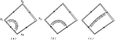
It is not hard to evaluate the integrals appearing in the three cases above Drummond:2007aua :
-
•
Integrals of type vanish identically, being proportional to the square of the corresponding momentum. Consider :
(4.11) since the .
-
•
Integrals of type are divergent, since they capture the expectation value of a cusp Wilson loop (with sides of finite extent). Consider for example ; it yields
(4.12) where is a two-particle momentum invariant. The double pole in arises from integration in the vicinity of the cusp at the point . As mentioned before, the formal similarity of this calculation with that in position space suggests identifying with an ultraviolet regulator. This identification will be reinterpreted to account for the fact that in dual “configuration” space short distances are identified with small energies.
-
•
Integrals of type are finite and thus can be evaluated directly in four dimensions. For instance, yields:
(4.13) (4.14) (4.15) Similarly to the integrals of type , and .
All other integrals can be obtained from and by simple relabeling of the momenta. It is not hard to see that the features of the three types of integrals described here are quite general, regardless of the number of sides of the polygon; integrals of type always vanish, integrals of type contain only double-poles (and the associated momentum dependence) and diagrams of type are completely finite.
The complete one-loop contribution to the expectation value of the four-sided Wilson loop can now be pieced together. Inserting (4.11), (4.12), (4.15) and their relabeled versions into (4.10) leads to
| (4.16) |
where the divergent part, denoted by , arises entirely from integrals of type and it reads
| (4.17) |
An important point to note is the similarity of this divergence and the expression of the logarithm of the Sudakov form factor (2.42) with ; this should not be surprising, in light of the fact that part of the Sudakov form factor may be computed in the eikonal approximation. The similarity may be sharpened by the following identifications:
| (4.18) |
The first relation captures the fact that while from the standpoint of the calculation described here the singularities have a short distance nature, they are in fact due to gluons with low energy and/or low transverse momentum when viewed from the position space perspective. The second relation, inverting the unit scale of dimensional regularization, is a reflection of the fact that the coordinates of this configuration space have positive mass dimension.
A remarkable feature of equation (4.16) is that its finite part, defined as the remainder after the subtraction of all infrared divergences and of the associated terms depending on the unit scale – i.e. in equation (4.17), reproduces up to an additive constant the finite part of the one-loop amplitude (2.84).
4.2.2 Higher polygons
The calculation of the expectation value of Wilson loops constructed on higher polygons bears a certain similarity with the expectation value of the four-sided loop. The curve is now given by where each segment () is parametrized as before . Similarly to the four-sided loop calculation, the result for the expectation value at one-loop is given in terms of three types of integrals whose generic types are shown (for a six-sided loop) in figure (24).
| (4.19) |
The main difference compared to the four-sided loop involves the diagram in figure 24(c) and is that at least one of the two momentum invariants that may be constructed from the coordinates of the endpoints of the edges connected by the gluon exchange (and not involving any of the momenta of the connected edges) is nonvanishing. One may consider treating separately the case of a vanishing invariant; it turns out however that this may be obtained smoothly from the general situation of two nonvanishing invariants.
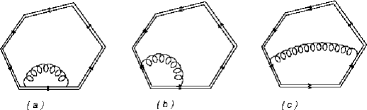
The diagrams in figures 24(a) and 24(b) are identical to those in figures 23(a) and 23(b); the first one vanishes identically () because the edges of the Wilson loop are light-like while second one yields434343Recall that .
| (4.20) |
Similarly to the integrals in figure 23(c), the integrals in figure 24(c) are finite and thus may be computed directly in four dimensions. Denoting by and the beginning vertex of the edges connected by the gluons and by and the corresponding momenta, the gluon propagator is a function of
| (4.21) |
The sum is nothing but the sum of momenta on one side of the edges connected by the gluon. Denoting it by and also introducing as the sum of momenta on the other side of the edges connected by the gluon, (such that ), and , it is not hard to find that
| (4.22) |
The resulting double-integral representation of the diagram shown in figure 24(c) is then
Upon integration BHT , it surprisingly yields the finite (and -independent) part of the easy two-mass box function introduced in section 2
| (4.24) | |||||
| (4.25) |
Note that the limits and are smooth; this justifies treating the configurations with as limits of the generic integrals .
Collecting all contributions to the expectation value of the -sided Wilson loop following (4.19) one finds BHT
| (4.26) |
with being an additive constant. Here is, up to the identifications (4.18), the appropriate sum of the logarithms of Sudakov form factors444444That is, is the sum of one-loop form factors evaluated on all adjacent two-particle invariants . Its explicit expression follows from (2.82) by replacing and with their one-loop values: and . and reproduces the finite part of the one-loop MHV amplitude (2.85)-(2.88). 454545 The relation between Wilson loops and scattering amplitudes may be extended, at one-loop level, to an “integral-by-integral” identity. As discussed in BHNST_gravity , one may pick a gauge in the dimensionally regularized theory in which the diagrams 24(b) also vanishes identically. Then, the complete contribution to the expectation value of the Wilson loop comes from the integrals 24(c) each of which, in this gauge, equals one easy two-mass box function.
It is interesting that in Feynman gauge, used in the preceeding calculation, there is such a clean separation of the divergent and the finite contributions to the expectation value of the Wilson loop. As we will see in later sections, this separation does not survive at higher loops. It would be interesting to identify a different gauge which realizes such a separation to all orders in perturbation theory.
Before proceeding let us remark that, from the details described above following Drummond:2007aua , BHT , it is apparent that the one-loop expectation value of the Wilson loop under discussion is entirely independent on the matter content of the gauge theory it is evaluated in. This suggests that, at least at one-loop level, MHV scattering amplitudes in SYM theory capture a universal structure of all gauge theories. Since the BDS ansatz is constructed – up to the explicit expression of the cusp anomaly – from the one-loop amplitude, this also suggests that the BDS ansatz captures a universal part of scattering amplitudes in all gauge theories – the part determined by infrared singularities and dual conformal invariance.
4.3 A conformal Ward identity
Wilson loops are generically not invariant under coordinate transformations, since the latter changes the contour defining them; if the Lagrangian is invariant and if the Wilson loop is well-defined (finite), then one finds instead that
| (4.27) |
where is the image of curve under this coordinate transformations.
By restricting the class of coordinate transformations to the conformal group it is possible to find more interesting information. While being operators of vanishing classical dimension, generic Wilson loops do not enjoy definite conformal properties, because the contour defining them changes under general conformal transformations. Light-like Wilson loops are however special due to the fact that conformal transformations preserve the light-cone up to perhaps dilatations. In the case at hand the contour is composed of light-like segments . It is not hard to check that an inversion transformation preserves this property:
| (4.28) | |||
| (4.29) |
Thus, the light-like polygons used to construct the Wilson loops related to scattering amplitudes are invariant under inversion. They are of course not invariant under translations and Lorentz transformations, but their expectation value is, since it depends only on the norm of the difference of coordinates of the endpoints of the edges. The same then holds true for special conformal transformations.
Thus, since the SYM theory is invariant under conformal transformations, if the expectation value of light-like polygonal Wilson loops were finite and well defined in four dimensions, they would also be invariant under conformal transformations.
| (4.30) |
since the action compensates464646I.e. a coordinate transformation is necessary. for the changes in the contour under transformations. 474747This conclusion holds despite the fact that the Wilson loops are defined in a configuration space related to momentum space rather than in the usual position space. One only needs to interpret the conformal group acting on this configuration space – in this case the dual conformal group.
As we have seen previously however, the light-like polygonal Wilson loops require regularization both because of the presence of cusps as well as because of the presence of light-like edges which also lead to collinear singularities. Any regularization breaks (dual) conformal invariance and thus potentially leads to anomalies. They were studied in Drummond:2007au ; in the following we will review the results obtained there.
4.3.1 General Properties of Cusp Singularities
A general feature of the polygonal Wilson loops conjecturally related to MHV scattering amplitudes is the presence of cusps. As we have seen in explicit calculations, their presence combined with the fact that the edges are light-like leads to an short distance singularity at one-loop.484848We remind the reader that in the present context the distance is “short” in the dual momentum space. The divergences arise from diagrams similar to those in figures 23(b) and 24(b); each of them contributes a factor (4.20). As a result, the divergent piece of the Wilson loop expectation value at one-loop has the form
| (4.31) |
with the position of the cusps and the indices are cyclic – . As alluded to earlier, these singularities arise in two regimes: when the gluon propagates a very short distance (which can happen only if the points connected by the gluon are near the cusp) and if the gluon propagates parallel to one of the edges of the cusp. They are in direct correspondence with the usual soft and collinear divergences which appear in one-loop scattering amplitudes. Indeed, if the gluon propagates a short distance in this configuration space its energy is very small; thus, this corresponds to the soft divergence (2.32). Analogously, if the gluon propagates parallel to one of the light-like edges, then its transverse momentum is very small and the corresponding singularity is analogous to a collinear divergence (2.33).
At higher loops the divergence structure is somewhat more complicated to disentangle; since in the same diagram one finds gluons attached to different segments and in different configurations, various soft and collinear regimes can be realized simultaneously, increasing the strength of the divergence. Additional divergences can arise from subintegrals whose external legs are not directly linked to the edges of the cusp. It nevertheless continues to be true that at higher loops all cusp singularities are a combination of soft and collinear ones (in the sense described above), similarly to the infrared singularities of scattering amplitudes; to -loop order, the singularities of light-like cusped Wilson loops are poles starting at order
| (4.32) |
Since from the standpoint of the evaluation of the Wilson loop expectation value these divergences are due to short distance effects, they may (and should) be renormalized. The renormalization properties of light-like Wilson loops have been extensively studied. An important result obtained in Korchemsky_Radyushkin is that Wilson loop operators are multiplicatively renormalized. In other words, divergences may be subtracted recursively and, after subtraction of all subdivergences, the remaining overall divergence is local and can also be subtracted by a counterterm, i.e.
| (4.33) |
where is finite as the regulator is removed while contains all divergences. 494949 In general, singularities in the expectation value of Wilson loops arise due to the presence of cusps. For a multi-cusped light-like Wilson loop the relation (4.33) generalizes in the obvious way . The structure of the divergent factor was analyzed in detail; the result obtained in Korchemskaya:1992je , Bassetto:1993xd is that cusp singularities exponentiate and the divergent factor has the special form
| (4.34) |
with the expansion coefficients of the cusp anomalous dimension (cf. equation (2.38)) and the so-called cusp collinear anomalous dimension, defined in the adjoint representation of . The first few coefficients of the weak coupling expansion of are shown in (2.44) while the first term in the expansion of the cusp collinear anomalous dimension is
| (4.35) |
Integrability allows the construction of an integral equation BES determining the cusp anomaly or universal scaling function to all orders in a weak (and/or strong) coupling expansion. It would be interesting to construct a similar equation for and/or . 505050It has been argued in Dixon_Magnea_Sterman that and are related by a scheme-independent multiple of the first subleading term in the large spin expansion of the anomalous dimension of twist-two operators.
The structure of cusp divergences implies that the logarithm of the expectation value of the light-like Wilson loops conjecturally related to MHV amplitudes may be written as
| (4.36) |
where is a finite contribution independent on . This structure matches the gauge theory expectations for the logarithm of the rescaled MHV amplitudes . In fact, the universality of infrared divergences, emphasized by the soft and collinear factorization and exponentiation theorem and by the discussion above, suggests that if non-MHV amplitudes are captured by some types of Wilson loops, then these loops necessarily must exhibit cusps.
4.3.2 Conformal properties of light-like Wilson loops
On general grounds, when a symmetry is broken by a regulator it may develop anomalies at the quantum level. They typically appear in the form of the product between a factor vanishing as the regulator is removed and a factor that would diverge in the same limit. Wilson loops in dimensional regularization could (and, as we will see following Drummond:2007au , actually do) exhibit such anomalies in (dual) dilatation and (dual) special conformal transformations.
Dimensional regularization preserves the dimension of fields due to the introduction of the unit scale :
| (4.37) |
where and we suppressed terms in the Lagrangian which have other fields besides gluons. The fact that the dimension of fields is unchanged implies that in the regularized theory the Wilson loop operator (4.3) continues to be conformally invariant up to a coordinate transformation. Both the Lagrangian and the integration measure relating it to the action transform homogeneously under this coordinate transformation; in four dimensions the action is invariant. A -dimensional integration measure breaks this invariance and induces an violation of dual conformal invariance (more precisely, it is no longer invariant under dilatations and conformal boosts). In the path integral evaluation of the Wilson loop expectation value this leads to an anomaly under these transformations.
The existence of anomalies may be captured systematically in several different ways. In the current context the most efficient one is through a Ward identity whose form – if the regulator preserved dilatations and conformal boosts – would be
| (4.38) |
the anomalies will appear as inhomogeneous terms on the right hand side of these equations. The starting point in the derivation of the relevant anomalies would be to perform the relevant transformations on the action in the presence of the regulator. It is possible however to bypass this step515151 The following arguments may, of course, be checked using the conformal transformations of SYM fields, denoted collectively by : (4.39) here are the Lorentz generators: . by recalling that the action is invariant if and that the transformation rules for fundamental fields does not depend explicitly on the dimension. It thus follows that the Lagrangian transforms homogeneously with weight four:
| (4.40) |
Thus, under infinitesimal dilatations, the regularized action transforms as525252In the presence of the regulator the measure transforms as . Using and assuming that for an infinitesimal transformation is small, it is easy to find (4.41) upon expansion in .
| (4.41) |
From here one immediately concludes that
| (4.42) |
Because of the presence of divergences in the correlation function on the right hand side, it is not possible to set it to zero, despite its manifest proportionality to the dimensional regulator. In light of the discussion of singularities of cusped Wilson loops, one may in fact wonder whether a single power of is sufficient to render the right hand side finite. As we shall see, this is indeed the case.
A similar analysis yields an expression for the special conformal transformations of the expectation value of the Wilson loop. The derivative part of special conformal transformations is a genuine invariance of the Lagrangian; this may be seen from the fact that the transformation of the measure is trivial. Special conformal transformations also exhibit a dilatation component, whose presence is necessary for the closure of the algebra. Since the conformal boost generators carry a vector index, their dilatation component must be multiplied by . Thus, up to this factor of the coordinate, the action of these generators on the Wilson loop is the same as that of the dilatation generator:
| (4.43) |
The precise normalization may be derived by making use of the commutation relation or from the transformation rules in footnote 51. Similarly to (4.42), the presence of divergences prevents at this stage setting on the right hand side of the equation above; these terms are the origin of the conformal boost anomaly Drummond:2007au .
The renormalization properties of Wilson loops (4.33) suggest that it would be convenient to organize the equations (4.42) and (4.43) such that the divergent and finite parts are separated. Thus, a convenient rewriting should involve the logarithm of the expectation value of the Wilson loop by simply dividing by :
| (4.44) | |||
| (4.45) |
where the left hand side is written in terms of logarithms because and are linear differential operators. The explicit multiplication by on the right hand side implies that only the divergent terms need to be evaluated since only they can contribute to this product in the limit.
The right hand side of the equations (4.44) and (4.45) have been explicitly evaluated at one-loop order and the result extended to all loops in Drummond:2007au . For the most part, the details are common between the two equations: one first evaluates as a function of the insertion point and then reconstructs the two inhomogeneous terms above by direct integration.
To lowest nontrivial order, is simply given by the same matrix element as the leading contribution to the expectation value of the Wilson loop with an additional insertion of the Lagrangian, the only contributing part of which is the gluon kinetic term
| (4.46) |
This insertion slightly modifies the diagrams in figure 24 to those in figure 25. As we have seen, in the absence of additional insertions, only the diagram 24(b) develops singularities in Feynman gauge. The same continues to hold here and only the diagram 25(b) develops singularities in Feynman gauge.

The final result for this expectation value, obtained in Drummond:2007au , is
| (4.47) |
where the function
| (4.48) |
is first term in the weak coupling expansion of a function . Not entirely unexpectedly, the double-pole in (4.47) is localized at the cusps; the simple poles in (4.47) receive contributions both from cusps as well as from the edges. There is thus a similarity between the origin of various pole terms at weak and strong coupling (cf. section 3.3, up to the change of regularization from cut-off to dimensional regularization).
Upon integration with and without the weight in equations (4.44) and (4.45) the contribution of simplifies to
| (4.49) | |||||
| (4.50) |
upon summation over the labels of the cusps, the contribution of to the right hand side of the Ward identity for (dual) conformal boosts vanishes as well. Thus, collecting everything, it is easy to find that
| (4.51) | |||||
| (4.52) |
These equations may be turned into an anomalous Ward identities for the (logarithm of the) finite factor of the Wilson loop expectation value. Substituting the expression of in terms of and – – and working out the action of and on , one quickly finds that
| (4.53) | |||||
| (4.54) |
The complete cancellation of singularities also identifies the numerical coefficient of the leading singularity on the right hand side of (4.51) with the leading term in the weak coupling expansion of the cusp anomalous dimension. This observation was used in Drummond:2007au to gain information on the all-loop structure of the anomaly.
4.3.3 An all-loop generalization of the conformal Ward identity
Unlike axial anomalies, the anomalies of the dual conformal symmetry are not one-loop exact. It is possible, though not completely straightforward, to generalize to higher loops the calculation described in the previous section. A key point which makes the calculations tractable is that, as repeatedly mentioned above, the complete contribution to the anomaly is governed by the singular terms in the expectation value .
Information on the structure of anomaly can be gained from the observations made before – that at one loop the coefficient of the leading pole is the one-loop cusp anomaly – and from the fact that the Ward identity for the finite part of the Wilson loop should relate finite quantities. From here it seems reasonable to conclude that the coefficient of the leading singularity of should in fact be proportional to first logarithmic integral of the cusp anomaly (with the proportionality coefficient determined by the one-loop calculation) and that the coefficient of the local term should also contain :
The structure of the coefficient of guarantees that, as desired, all singularities cancel in the action of and on .
Ref.Drummond:2007au argued that, order by order in the weak coupling expansion, the contribution of to the Ward identity vanishes identically upon integration over the insertion point and summation over cusp labels. The argument is based on dimensional analysis, the scheme independence of and the fact that the form of is, up to its arguments, independent of the cusp it originates from.535353Independently of these arguments, it is possible to show explicitly that a calculation which strengthens the arguments of Drummond:2007au .
Inserting (4.3.3) into the first equation of (4.51) and making use of the vanishing arguments for the contributions of one finds the all-order Ward identities for dilatation and conformal boosts
| (4.56) | |||||
| (4.57) |
Similarly to the one-loop calculation in the previous section, it is useful to recast these equations as constraints on the finite factor in (4.33). As expected and desired, all singularities cancel and the regulator can be removed (). Thus, (4.56) and (4.57) become
| (4.58) | |||||
| (4.59) |
The first equation implies that the finite part of the expectation value of cusped Wilson loops discussed here are functions of dimensionless, scale invariant ratios of products of cusp coordinates . The same conclusion may be reached on dimensional grounds, making use of the fact that, in the presence of the regulator, depends on the unit scale of dimensional regularization. Then,
| (4.60) |
which becomes (4.58) upon use of (4.33). The consequences of the conformal boost Ward identity will be discussed in the next section; not surprisingly, the results reproduce the structure of constraints on scattering amplitudes following from dual conformal invariance.
4.3.4 Constraints on expectation values of Wilson loops
As we have seen previously, the equation (4.58) implies a relatively simple constraint on the finite part of the Wilson loop. The Ward identity for conformal boosts requires further analysis.
The notation may be slightly simplified by making use of the maximal nonabelian exponentiation theorem max_nonabelian_exp1 , max_nonabelian_exp2 , max_nonabelian_exp3 which states that the expectation value of Wilson loops have a natural exponential structure and the exponent itself has an diagrammatic interpretation in that it receives contributions only from the Feynman diagrams which are two-particle irreducible. From this standpoint it is perhaps more natural to replace by its logarithm
| (4.61) |
The reason for introducing the factor of the cusp anomaly is that the right hand side of (4.59) also exhibits a similar overall factor and thus the resulting equation does not contain any further explicit coupling constant dependence:
| (4.62) |
As usual, the solution to this type of equation is a sum between a solution of the inhomogeneous equation and a general solution of the homogeneous one. Because of its lack of coupling constant dependence, the equation (4.62) implies that the solution to the inhomogeneous equation is determined by a one-loop calculation. It is thus clear that, up to the coupling constant dependence, is just the one-loop expectation value of the -sided Wilson loop.545454It is quite remarkable that, interpreting the cusp anomalous dimension as the “physical” coupling constant makes the anomaly of dual conformal conformal boosts into an one-loop-exact quantity. This is reminiscent of suggestions in reference physical_coupling1 , physical_coupling2 .
The calculations in sections 4.2.1 and 4.2.2 imply then that
| (4.63) |
with and given by equations 2.84 and 2.85-2.88, respectively. It is indeed possible to check Drummond:2007au that these expressions solve the equation (4.62).
To this solution one should add a solution to the homogeneous version of equation (4.62) (i.e. the equation with the right hand side removed). Instead of finding the general solution by directly solving this differential equation, it is more convenient to make use of the fact that conformal boosts are just a combination of inversion and translation – – and construct inversion and translation invariants known as conformal cross-ratios which also appeared in our discussion of conformal properties of scattering amplitudes in section 2.5. This strategy is extensively applied in two-dimensional conformal field theories; in four dimensional theories it was initially applied, in a related context, in broadhurst .
As we briefly mentioned in section 2.4.1, inversion transformations act as
| (4.64) |
Thus, using the fact that , inversion and translation invariants are constructed from the coordinates of any four cusps whose labels differ ( the number of sides of the polygon) by at least two units. All relevant invariants may be identified by choosing four unordered labels and constructing
| (4.65) |
reordering of the labels may lead to different invariants corresponding to the same choice of cusps. The solution to the homogeneous form of the equation (4.62) is then an arbitrary function of all possible such conformal cross-ratios and of the coupling constant .
Clearly, the cross-ratios (4.65) are even under parity transformations. It is also possible to construct dual conformal invariants which are parity-odd. Products of an even numbers of such quantities are expressible in terms of the cross-ratios (4.65). We are assuming throughout that the solution to the anomalous Ward identity does not contain terms linear in such parity-odd invariants.
Not surprisingly, the number of invariants depends strongly on the number of cusps. Simple counting implies that for and no such conformal ratios may be constructed; thus, the only solution of the homogeneous equation (4.62) for four- and five-sided polygons is just a constant. Thus,
| (4.66) |
Conformal cross-ratios exist for polygons of at least six sides. The minimum number of invariants occurs for ; it is trivial to check that
| (4.67) |
are indeed solutions of the homogeneous equation (4.62) and, because of the linearity of , so is any function of them. Thus,
| (4.68) |
where we denote by the solution of the non-anomalous Ward identity which is necessary to relate (4.63) to the expectation value of the six-sided Wilson loop. A similar function may be defined for Wilson loops with an arbitrary number of edges
| (4.69) |
and represents the Wilson loop analog of the remainder function capturing the departure of scattering amplitudes from the BDS ansatz (cf. section 2.5).555555The first argument of denotes the set of all conformal cross-ratios that can be constructed from the coordinates of the cusps.
4.4 Higher-loop tests of the amplitude/Wilson loop relation
The discussion in previous sections exposes a relation between two apparently different quantities: MHV gluon scattering amplitudes in SYM theory and the expectation value of Wilson loops constructed in a special way from light-like segments. Manipulations using -duality transformations for strings in suggest that this is indeed the case at strong coupling (cf. section 3). At weak coupling we have seen evidence for this relation at one-loop level and we will see further two-loop evidence in the next section. Before proceeding with describing these calculations DHKS1_2loop , Drummond:2007au , DHKS3_2loop , DHKS4_2loop , let us pause and discuss the general structure of both amplitudes and Wilson loop expectation values which have emerged from our symmetry considerations.
The structure of MHV scattering amplitudes follows from the BDS ansatz, explicit calculations and the assumption that the dual conformal symmetry observed at low orders in perturbation theory holds to all orders in perturbation theory: 565656As mentioned previously in section 2, in the absence of an explicit proof, this assumption must to be tested by explicit calculations.
| (4.70) |
where is the rescaled one-loop amplitude, is a function of the ’t Hooft couplings and all conformal ratios consistent with the kinematics of the process and and are functions that are independent of the kinematics and the number of gluons. The first two and last two terms above are part of the BDS ansatz while the remainder function captures the potential departures from it. It is important to stress that and thus the BDS ansatz holds true in these cases.
The structure of the expectation value of light-like cusped Wilson loops follows, as seen in the previous section, from explicit calculations and dual conformal invariance:
| (4.71) |
where is, up to a factor of the cusp anomaly, the one-loop expectation value of the Wilson loop, is a function of the ’t Hooft couplings and all conformal ratios consistent with the light-like nature of the loop and and are functions that are independent of the kinematics or the number of edges. Explicit computations show that . It is also important to mention that this separation of the divergent part of the logarithm of the Wilson loop expectation value from its finite part is consistent with the strong coupling analysis described in section 3.
If both the amplitude/Wilson loop relation as well as the BDS ansatz were indeed to hold, then together they would imply that the logarithm of the expectation value of the light-like cusped Wilson loops, naturally given by the maximal nonabelian exponentiation theorem in terms of Feynman diagrams, would equal up to a factor of the cusp anomaly the one-loop expectation values of the same light-like cusped Wilson loops. This nontrivial statement holds for four- and five-sided loops, as a consequence of dual conformal invariance which implies that the remainder functions are constants. As we will review in section 4.5.2, starting with six-sided loops this no longer holds, implying the existence of nontrivial remainder functions.
On the explicit expressions (4.70)-(4.71) one may take the strong coupling limit and contrast the result with the expectations stemming from the analysis in section 3. If the relation between Wilson loops and MHV amplitudes holds, then
| (4.72) |
One may further make use of the fact that to conclude that the two remainder functions and must be equal. It is however more instructive to temporarily leave equation (4.72) unchanged.
4.4.1 Rectangular configuration with a large number of gluons
To test the relation between Wilson loops and MHV amplitude at strong coupling in the form of the equation (4.72) it appears necessary, at least at first sight, to find the minimal surface corresponding to some -sided polygonal boundary conditions. As seen in section 3, such a construction is challenging for any number of sides larger than four. As we have discussed, agreement is guaranteed in this instance by dual conformal invariance.
A technically simpler construction corresponds to a relatively singular kinematics corresponding to infinitely many gluons with alternating positive and negative energies. In the dual configuration space this is represented by a sequence of light-like segments spanning a zigzag following a light-like rectangular contour of width and height , as shown in figure 26.

In the limit of a large number of edges and for very large and such that the contribution to the scale-invariant part of the result may be identified as being given by the same minimal surface that yields the quark-antiquark potential Rey:1998ik , Maldacena:1998im . Indeed, in this limit and for the purpose of the evaluation of the scale-invariant part of the area, the minimal surface corresponding to the zigzag boundary condition may be approximated by the minimal surface ending of the rectangle. It follows then Rey:1998ik , Maldacena:1998im that
| (4.73) |
This is the strong coupling limit of the scale-invariant part of the left hand side of the equation (4.72). The first term on the right hand side may be trivially computed, as it is given by the strong coupling limit of the cusp anomaly and the particular kinematic limit of the expectation value of the -sided Wilson loop at one-loop – i.e. by the scale-invariant part of the one-loop correction to the quark-antiquark potential:
| (4.74) |
where we used the fact that, as stated in (4.1), . Since this first term on the right hand side of the equation (4.72) does not reproduce the expression in equation (4.73), it follows that the remainder functions and/or are nontrivial functions of kinematic invariants575757It is worth mentioning that this reasoning was the first indication that the BDS ansatz departs from the true expression of scattering amplitudes. Additional evidence in the same direction comes from the analysis of the BFKL equation BLSA .. This is consistent with the observation in section 2 that is nontrivial. To strengthen this conclusion we will summarize in the next section the two-loop correction to the expectation value of light-like cusped Wilson loops.
4.5 Two loops and beyond
The arguments in the previous sections, leading to the conjectured relation between scattering amplitudes and light-like cusped Wilson loops, are very compelling. Dual conformal symmetry is, however, yet to be proven to be a symmetry of the (MHV) amplitudes. Thus, its presence and consequences need to be tested.
One way to explore further the scattering amplitudes/ Wilson loops equivalence is by comparing the results of explicit calculations on both sides. This includes both four- and five-point amplitudes and the corresponding Wilson loops. The rationale behind low-point calculations is to test the consequences of dual conformal invariance. In the following we review two-loop computations for the expectation value of light-like Wilson loops for four and six cusps585858The two-loop correction to the five-sided cusped Wilson loop was evaluated in Drummond:2007au .. The loop with is particularly important since, as we have already seen, it is the lowest number of edges for which the result is not fixed by conformal invariance and thus a remainder function can appear.
Both for and for the goal is to evaluate the expectation value (4.3) up to order . One may organize the contributions to the expectation value of the loop following the order in the expansion of the path-ordered exponential which participates in the calculation. To order there are are terms with two, three and four gauge fields:
| (4.75) | |||||
| (4.76) | |||||
where we used the notation . The two-gluon term contributed to the one-loop expectation value as well. To order some of the interaction terms in the Lagrangian become relevant. Indeed, to this order, the two-gluon term above combines with two three-field terms or one four-field term from the Lagrangian, while the three-gluon term above combines with a three-field term in .
As in the one-loop computation, all terms may be conveniently represented in terms of Feynman diagrams. Depending on the number of edges of the loop they may be further classified following the number of adjacent edges the gluons are attached to. Some of the diagrams which appear in all calculations are shown in figure 27. The diagrams 27(a) have the same topology as the one loop diagrams except that the gluon propagator is dressed with a self-energy insertion. The diagrams 27(b) contain three gluon propagators joined by a three-gluon vertex. Last, diagrams 27(c) do not contain any interaction terms from the Lagrangian.
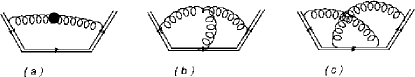
It is interesting to note that these diagrams are almost independent of the matter content of the theory. Indeed, all diagrams except the self-energy insertion receive contributions only from gauge fields. Moreover, the one-loop gluon self-energy insertions are very similar in all four-dimensional conformal field theories as fundamental role of the matter content at this order is to guarantee the vanishing of the beta function. A possible interpretation of this observation is that, similarly to the BDS ansatz, the expectation value of cusped Wilson loops captures a universal part of the physics of four-dimensional conformal field theories in general and of their scattering amplitudes in particular (a part which is nonetheless different from that captured by the BDS ansatz).
An important tool in higher-loop computations is the so called nonabelian exponentiation theorem max_nonabelian_exp1 , max_nonabelian_exp2 , max_nonabelian_exp3 . As mentioned previously, it states that the expectation value of Wilson loops has a natural exponential structure; the logarithm of is itself given in terms of Feynman diagrams which are a subset of the complete set of diagrams595959Up to a few planar diagrams with two gluon propagators contributing to . This subset is identified by the color factors:
| (4.78) |
where denotes the loops contribution to the expectation value of the Wilson loop and denotes the contribution to with the ”maximally nonabelian” color factor . Roughly, only the subset of loops diagrams with maximally interconnected gluon propagators contribute to . The examples in the following section will hopefully clarify this notion. To the first few orders in the loop expansion, , the maximally nonabelian factor is , but starting from four loops it is not expressible in terms of the Casimirs and max_nonabelian_exp2 , max_nonabelian_exp3 .
The diagrams with non-maximal color factor factorize in products of lower-loop contributions and, in the calculation of , may be identified with terms in the expansion of . From this perspective one may intuitively relate the appearance of maximal nonabelian color factors with two-particle irreducibility. To conclude these preparations, by using the nonabelian exponentiation theorem, is completely determined by the contribution to proportional to . 606060Indeed, by using the nonabelian exponentiation theorem we find that and , so the piece of proportional to is determined by the one loop correction.
4.5.1 Polygon with four cusps
The basic ingredients of two loops computations already appear when studying two loops corrections to the four cusps Wilson loop, so we begin by reviewing this calculation in some detail DHKS1_2loop . The complete set of diagrams, not making use of the nonabelian exponentiation theorem, is shown in figure 28.

It is not hard to argue that, similarly to their one-loop counterparts, two-loop diagrams with both ends of a gluon propagator on the same light-like edge vanish identically (essentially because they depends on a single momentum and no nonvanishing invariant may be constructed from it). They have not been included in figure 28. The properties of nonvanishing diagrams are summarized below DHKS1_2loop :
-
•
Diagrams with a single (dressed) gluon propagator are shown in fig. 28, (a) and (b). Their color factor is , and thus they contribute to . Both contain contain divergences due to the presence of the cusp, from the light-like edges and also intrinsic to the self-energy insertion. Their pole expansion takes the form and .
-
•
The color factor of diagrams with three gluon propagators joined by a interaction vertex, shown in figures 28, (c), (d) and (e), is also ; they therefore also contribute to . All of them are divergent and their pole expansion is , and . The strength of the leading singularity may be understood in terms of the number gluon propagators which may collapse at cusp singularities.
-
•
Non-planar diagrams with two gluon propagators, shown in figures 28(f)–(j), have a color factor equal to . Hence, the term proportional to , obtained by replacing , contributes to 616161Notice that the contribution of these diagrams to is suppressed in the large limit, however, their contribution to is not. Diagrams of type (g), (i) and (j) are finite, while diagrams and diverge as and . Similarly to the previous item, the strength of these singularities may be understood in terms of the number gluon propagators which may collapse at cusp singularities.
-
•
The planar diagram with iterated gluon propagators shown in figure 28(k) has as color factor. Therefore, this diagram does not contribute to . In fact, it combines with the terms proportional to ignored in the previous item to yield unrestricted integrals over the end-points of the two gluon propagators; these terms are nothing but the finite part of which is necessary to reconstruct .
It is possible to find analytic expressions for all the integrals shown in figure 28. Combining them in the appropriate permutations leads to an expression for :
| (4.79) |
Combining this and the expression for constructed in section 4.2.1 leads to an expression for the logarithm of the expectation value of the Wilson loop as a sum of a divergent term and a finite term, which matches the structure of equation (4.36)
| (4.80) |
The divergent and finite parts are
| (4.81) | |||
| (4.82) |
The identifications (4.18) imply that the leading pole of agrees with the general form of the infrared poles of scattering amplitudes (2.82). The subleading poles in the same equation, evaluated for the universal scaling function and -function of SYM, are also reproduced after a further -dependent redefinition of . The double-logarithm in the finite term reproduces the kinematic dependence of the finite part of the two loops MHV amplitude for four gluons (2.85). Its coefficient may be recognized as the two-loop cusp anomaly (2.44). In light of the constraints imposed by dual conformal invariance this agreement is not surprising; this calculation however shows the validity of higher-loop arguments based on it. 626262In Korchemskaya it was argued that a similar duality relation between the four point amplitude and the four edges Wilson loop holds also for QCD in the Regge limit.
4.5.2 Polygon with six cusps
As discussed at length in section 4.3.4, dual conformal symmetry is not sufficiently powerful to completely fix the expectation value of light-like Wilson loops with at least six cusps. The expectation value is instead fixed up to the addition of some function of conformal ratios and the coupling constant (cf. equation (4.69). Thus, the finite part of the logarithm of the six-sided loop (defined by ) is
| (4.83) |
where is the one-loop expectation value of the six-sided loop and is an arbitrary function of the coupling constant and the three nontrivial conformal cross-ratios which may be constructed from the coordinates of the six cusps (see equation (4.67)). Its loop expansion reads
| (4.84) |
By construction, the one-loop remainder function is at most a constant independent of the kinematics. The properties of the higher loop terms in (4.84) may be found (at the time of this writing) only by explicit calculations of the higher loop expectation value of the Wilson loop.
As for the four-sided loop, the calculation makes use of the nonabelian exponentiation theorem, which identifies, at the level of Feynman diagrams, the contributions to . It is however unclear whether the contributions to have by themselves a Feynman diagram interpretation.636363 One may attempt to identify them with the diagrams which do not exists for loops with four and five cusps. However, even the diagrams that do exists in those cases are structurally different since some of the differences of cusp coordinates are no longer light-like. It is therefore not clear whether such an identification is appropriate. Thus, the only available method of identifying is to first evaluate the complete two-loop contribution to and then subtract the divergences as well as the two-loop contribution of the first term in equation (4.83).
The calculation was carried out in DHKS3_2loop , DHKS4_2loop ; some of the diagram topologies contributing to are analogous to those discussed in section 4.5.1 (see however the differences pointed out in footnote 63). Others are completely different, due to the additional freedom provided by the existence of additional edges.
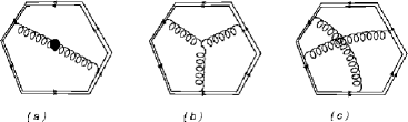
The calculation is technically more involved that that of the four- and five-sided polygon; the final result may currently be found only numerically. An immediate test of the result is that indeed the Wilson loop remainder function depends only on the three conformal cross-ratios, as the initial construction implies. Besides this consequence of dual conformal invariance, it is also possible to identify other properties of the and compare them with expectations based on the conjectured relation with MHV scattering amplitudes, as captured by the equation (4.72). Perhaps the main consequence of that equation is that in the Wilson loop analog of a collinear limit, consistency with the results for the expectation value of the five-sided loop requires that the Wilson loop remainder function should become a constant.646464This is analogous to the requirement that the amplitude remainder function vanishes in this limit.
The precise definition of collinear limit was described in equation (2.20). By inspecting the expressions of the cross-rations in equations (2.89) and (4.67) it is easy to see that any collinear limit corresponds to exactly one vanishing cross-ratio. Without loss of generality one may choose it to be . It is then not hard to see that, in this limit, the remaining cross-ratios are related by
| (4.85) |
With the notation , the Wilson loop remainder function should therefore behave as
| (4.86) |
independently of . Thorough numerical tests of this relation were carried out in DHKS3_2loop with the result that equation (4.86) does indeed hold. Figure 30 illustrates the numerical results 656565We thank the authors of Drummond:2007aua for providing us with this figure.. The constant value of was found in DHKS4_2loop to be
| (4.87) |
Due to the singular nature of collinear limits, the numerical error associated to this value () is larger than for generic kinematic configurations.
Figure 30 also implies that is not a constant away from the surface. As discussed in section 2.6, the same holds for the (MHV) amplitude remainder function . The comparison of the values of the two functions at selected kinematic points was carried out in BDKRSVV , DHKS4_2loop . To avoid any mismatch due to unaccounted constant shifts as well as loss of numerical precision it is convenient to compare the difference of remainder functions from a chosen reference point. A convenient one is the symmetric point in table 2.1 for which the conformal cross-ratios are
| (4.88) |
The differences between the amplitude and Wilson loop remainder functions at the points and at (denoted by and , respectively) are shown in table 4.1; the third column contains the difference of remainders for the amplitude, while the fourth column has the corresponding difference for the Wilson loop.
| kinematic point | |||
|---|---|---|---|
The agreement between the remainder functions for the six gluon amplitude and that of the six-sided Wilson loop shown by table 4.1 suggests that MHV amplitudes and Wilson loops continue to be related even when dual conformal invariance is not sufficiently restrictive to uniquely fix them.
By construction, the remainder function for the six-gluon MHV amplitude vanishes in all collinear limits. Using the constant value (4.87) one may define a Wilson loop reminder with similar vanishing properties. Such a remainder function enforces the fact that all singularities as well as the finite terms related to them are accounted for by the solution of the anomalous Ward identity. It is worth mentioning that this remainder function reproduces the amplitude one without additional subtractions.
5 Outlook
Scattering amplitudes remain one of the basic ingredients in our understanding of quantum field theories. They are usually evaluated order by order in a weakly-coupled perturbation theory and it is rarely the case that the resulting series can be constructed and resummed to all orders in perturbation theory, even only in the planar limit. The SYM theory is perhaps special in this respect, being sufficiently simple to make higher order calculations feasible yet being sufficiently nontrivial for the resulting scattering matrix to (apparently) contain nontrivial dynamical information.
We have described techniques which allow, in SYM, efficient higher-loop and higher multiplicity calculations. Though not reviewed here, some of these techniques have been extended to phenomenologically-relevant theories, such as QCD (for a review see e.g. Bern:2007dw ). General properties of infrared singularities together with explicit higher loop calculations led to the formulation of the BDS ansatz, expressing all higher-loop MHV amplitudes in terms of their one-loop expressions.
In the strong coupling regime, the AdS/CFT duality suggests, through the use of T-duality, that partial amplitudes may be evaluated as the regularized area of the minimal surface ending on a special light-like polygon whose specific properties depend on the particles being scattered. Quite remarkably, explicit calculations show that this relation holds at weak coupling as well. While explicit higher-loop high-multiplicity calculations turn out to depart from existing conjectures for the resummation of the perturbative series for planar MHV amplitudes, they reproduce the results of Wilson loop calculations.
An important concept behind both weak- and strong-coupling amplitude calculations in SYM is that of dual conformal invariance. Initially observed in explicit results for scattering amplitudes, its origin remains unclear and its presence not proven to all orders in perturbation theory at the level of scattering amplitudes. It is however an almost manifest symmetry of Wilson loop expectation values. This symmetry is sufficiently powerful to uniquely fix the expressions of four- and five-point amplitudes to all orders in perturbation theory if its presence is assumed to all orders in perturbation theory. The resulting expressions reproduce the BDS ansatz for four and five particle processes.
The full consequences and implications of the developments reviewed here are yet to emerge and many questions, which will undoubtedly contribute in this direction, remain to be addressed. Some of them are included here:
-
•
Despite partial progress outlined in section 3.5, the construction of minimal surfaces describing the scattering of more than four gluons is still lacking. Such solutions, or at least an expression for their regularized area, may provide valuable input for understanding the iteration relations at strong coupling. Up to a choice of boundary conditions, the dynamics of strings in is described by an integrable two-dimensional field theory BPR , Wadia . It would be potentially profitable to understand the consequences of integrability for the construction of minimal surfaces in this space. While it is not clear whether the integrability of the worldsheet theory survives in the presence of the dimensional regulator, integrability at may suffice to find the regularized area of the minimal surface without explicitly constructing the solution.
-
•
Besides scattering processes, the strategy described in section 3 may be used to argue that the overlap between some composite operator and some multi-gluon state also has a minimal surface interpretation. Physically, this overlap has the interpretation of the decay amplitude of a colorless scalar (with particular couplings) into gluons. Minimal surfaces with this interpretation are not known even in the simplest cases. Besides their obvious interpretation in terms of decay amplitudes, understanding in detail such processes may also lead to understanding the calculations of anomalous dimensions of short operators on the string theory side of the AdS/CFT correspondence.
-
•
Besides dependence on momentum invariants, scattering amplitudes are also sensitive to the polarization (helicity) of the scattering states. While present if the calculation of scattering amplitudes is organized in terms of open-string vertex operators,this information is lost in the map to light-like Wilson loops. It would be very interesting to understand whether polarization information may be encoded in Wilson loop language. Attempts in this direction have appeared in McGreevy_Sever_pol , based on earlier considerations of ref. polyakov_amplitudes . In a similar vein, the Wilson loop/amplitude relation should map the loop equation obeyed by Wilson loops into apparently nontrivial constraints on scattering amplitudes. It would be interesting to understand their relevance.
-
•
As reviewed in section 3, the evaluation of corrections to the expectation value of the four-sided Wilson loop at strong coupling remains elusive. Calculations carried out in Kruczenski:2007cy suggest that the definition of the strong coupling version of dimensional regularization is subtle beyond classical level. While dimensional regularization remains the ideal choice for comparison with weak coupling calculations, intuition on the structure of the answer may be gained by considering alternative regularization schemes, such as that through a radial cut-off.
-
•
A second set of corrections to the leading order strong coupling calculation of scattering amplitudes amounts to relaxing the requirement that the saddle-point surface (in the presentation of the amplitude in terms of vertex operators) has disk topology. Such higher genus corrections translates into nonplanar corrections to the planar scattering amplitudes. It is an interesting question whether such calculations have a Wilson loop counterpart. It would be very interesting to understand whether dual conformal symmetry is present in any one of these calculations and, if not, what is the origin of its breaking.
-
•
In section 3.5 we have briefly summarized attempts of extending the strong coupling relation between Wilson loops and scattering amplitudes to less supersymmetric and/or non-conformally invariant situations. It seems important to complete this program, as it may provide valuable clues for extending the strong coupling calculations of scattering amplitudes to other, perhaps more phenomenologically-relevant theories.
-
•
While the existence of a dual conformal invariance for scattering amplitudes is beyond doubt at low orders in perturbation theory, it remains to be proven whether SYM exhibits this symmetry to all orders in the coupling constant expansion. Establishing it may constitute a step towards understanding the complete relation between amplitudes and Wilson loop expectation values. It would be equally interesting to extent this equivalence (initially formulated for MHV amplitudes) to non-MHV amplitudes. From a field theory standpoint little is known about such amplitudes beyond leading order, where they are given in terms of pseudo-conformal integrals with spinor-dependent coefficients. The dual conformal properties of next-to-MHV amplitudes have been discussed in DHKS_super , GK_ES_Paris . A supersymmetric generalization of dual conformal transformations played an important role in this discussion. At strong coupling, similar supersymmetric generalizations of dual conformal symmetries have been discussed in NB_Paris , BRTW , NBJM . The analysis described there also exposes a close relation between the generators of the dual (super)conformal group and the hidden (non-local) integrals of motion of the world sheet theory in the original AdSS5 (i.e. the worldsheet theory prior to the T-duality transformations relating scattering amplitudes and Wilson loops). The full implications of this relation remain to be uncovered.
-
•
Scattering amplitudes and Wilson loops are logically disconnected quantities. The existence of a close relation between MHV amplitudes and light-like cusped Wilson loops hints to the existence of new symmetries which connect (and perhaps uniquely determine) both quantities.
-
•
While numerical comparison shows that the remainder functions are the same in the amplitude and Wilson loop calculations, it should prove interesting to construct an analytic expression for these remainders. (It is worth mentioning that the Wilson loop approach yields apparently simpler integrals.) Such expressions may hold a key towards understanding the general structures of MHV amplitudes and to their generalization to all values of the coupling constant.
It is clear that additional structure, waiting to be uncovered, is present in SYM and that it may be sufficiently powerful to completely determine, at least in some sectors, the kinematic dependence of the scattering matrix of the theory.
Acknowledgments
L.F.A. thanks J. Maldacena and R.R. thanks Z. Bern, L. Dixon, D. Kosower, M. Kruczensky, M. Spradlin, A. Tirziu, A.Tseytlin, C. Vergu and A. Volovich, for collaboration on the topics reviewed here. We would like to thank Z. Bern, D. Kosover, J. Maldacena, G. Korchemsky, A. Tseytlin and especially L. Dixon for valuable discussions, suggestions and comments on the draft. We would also like to thank A. Sever, N. Berkovits, J. de Boer, P. Caputa, J. J. Carrasco, J. Henn, P. Heslop, V. Khoze, A. Murugan, E. Sokatchev and G. Travaglini for discussions. RR thanks the ETH in Zurich for hospitality during the programme “QCD and Strings”. The work of LFA is supported by VENI grant 680-47-113 while the work of R.R. is supported in part by the US National Science Foundation under grant PHY-0608114 and the A. P. Sloan Foundation.
References
References
- [1] N. Beisert and M. Staudacher, “Long-range PSU Bethe ansaetze for gauge theory and strings,” Nucl. Phys. B 727, 1 (2005) [arXiv:hep-th/0504190].
- [2] N. Beisert, R. Hernandez and E. Lopez, “A crossing-symmetric phase for AdS(5) x S**5 strings,” JHEP 0611, 070 (2006) [arXiv:hep-th/0609044].
- [3] N. Beisert, B. Eden and M. Staudacher, “Transcendentality and crossing,” J. Stat. Mech. 0701, P021 (2007) [arXiv:hep-th/0610251].
- [4] Z. Bern, J. J. M. Carrasco, H. Johansson and D. A. Kosower, “Maximally supersymmetric planar Yang-Mills amplitudes at five loops,” Phys. Rev. D 76, 125020 (2007) [arXiv:0705.1864 [hep-th]].
- [5] J. M. Maldacena, “The large N limit of superconformal field theories and supergravity,” Adv. Theor. Math. Phys. 2 (1998) 231 [Int. J. Theor. Phys. 38 (1999) 1113] [arXiv:hep-th/9711200].
- [6] S. S. Gubser, I. R. Klebanov and A. M. Polyakov, “Gauge theory correlators from non-critical string theory,” Phys. Lett. B 428, 105 (1998) [arXiv:hep-th/9802109].
- [7] E. Witten, “Anti-de Sitter space and holography,” Adv. Theor. Math. Phys. 2, 253 (1998) [arXiv:hep-th/9802150].
- [8] O. Aharony, S. S. Gubser, J. M. Maldacena, H. Ooguri and Y. Oz, “Large N field theories, string theory and gravity,” Phys. Rept. 323 (2000) 183 [arXiv:hep-th/9905111].
- [9] L. J. Dixon, “Gluon scattering in N=4 super-Yang-Mills theory from weak to strong coupling,” arXiv:0803.2475 [hep-th].
- [10] L. F. Alday, “Lectures on Scattering Amplitudes via AdS/CFT,” arXiv:0804.0951 [hep-th].
- [11] F. A. Berends and W. T. Giele, “Recursive Calculations for Processes with n Gluons,” Nucl. Phys. B 306, 759 (1988).
- [12] F. Cachazo, P. Svrcek and E. Witten, “MHV vertices and tree amplitudes in gauge theory,” JHEP 0409, 006 (2004) [arXiv:hep-th/0403047].
- [13] A. Brandhuber, B. J. Spence and G. Travaglini, “One-loop gauge theory amplitudes in N = 4 super Yang-Mills from MHV vertices,” Nucl. Phys. B 706 (2005) 150 [arXiv:hep-th/0407214].
- [14] R. Britto, F. Cachazo and B. Feng, “New recursion relations for tree amplitudes of gluons,” Nucl. Phys. B 715, 499 (2005) [arXiv:hep-th/0412308];
- [15] R. Britto, F. Cachazo, B. Feng and E. Witten, “Direct proof of tree-level recursion relation in Yang-Mills theory,” Phys. Rev. Lett. 94, 181602 (2005) [arXiv:hep-th/0501052].
- [16] Z. Bern, L. J. Dixon and D. A. Kosower, “On-Shell Methods in Perturbative QCD,” Annals Phys. 322, 1587 (2007) [arXiv:0704.2798 [hep-ph]].
- [17] L. J. Dixon, “Calculating scattering amplitudes efficiently,” arXiv:hep-ph/9601359.
- [18] F. Cachazo and P. Svrcek, “Lectures on twistor strings and perturbative Yang-Mills theory,” PoS RTN2005, 004 (2005) [arXiv:hep-th/0504194].
- [19] Z. Bern and D. A. Kosower, “Color Decomposition Of One Loop Amplitudes In Gauge Theories,” Nucl. Phys. B 362, 389 (1991).
- [20] M. L. Mangano, S. J. Parke and Z. Xu, “Duality And Multi-Gluon Scattering,” Nucl. Phys. B 298, 653 (1988).
- [21] R. Roiban, M. Spradlin and A. Volovich, “On the tree-level S-matrix of Yang-Mills theory,” Phys. Rev. D 70, 026009 (2004) [arXiv:hep-th/0403190].
- [22] D. A. Kosower, “All-order collinear behavior in gauge theories,” Nucl. Phys. B 552, 319 (1999) [arXiv:hep-ph/9901201].
- [23] Z. Bern and G. Chalmers, “Factorization in one loop gauge theory,” Nucl. Phys. B 447, 465 (1995) [arXiv:hep-ph/9503236].
- [24] M. T. Grisaru and H. N. Pendleton, “Some Properties Of Scattering Amplitudes In Supersymmetric Theories,” Nucl. Phys. B 124 (1977) 81.
- [25] S. J. Parke and T. R. Taylor, “An Amplitude for Gluon Scattering,” Phys. Rev. Lett. 56, 2459 (1986);
- [26] F. A. Berends and W. T. Giele, “Recursive Calculations for Processes with n Gluons,” Nucl. Phys. B 306, 759 (1988).
- [27] R. Akhoury, “Mass Divergences Of Wide Angle Scattering Amplitudes,” Phys. Rev. D 19, 1250 (1979);
- [28] A. H. Mueller, “On The Asymptotic Behavior Of The Sudakov Form-Factor,” Phys. Rev. D 20, 2037 (1979);
- [29] J. C. Collins, “Algorithm To Compute Corrections To The Sudakov Form-Factor,” Phys. Rev. D 22, 1478 (1980);
- [30] A. Sen, “Asymptotic Behavior Of The Sudakov Form-Factor In QCD,” Phys. Rev. D 24, 3281 (1981);
- [31] G. Sterman, “Summation of Large Corrections to Short Distance Hadronic Cross-Sections,” Nucl. Phys. B 281, 310 (1987);
- [32] J. Botts and G. Sterman, “Sudakov Effects in Hadron Hadron Elastic Scattering,” Phys. Lett. B 224, 201 (1989) [Erratum-ibid. B 227, 501 (1989)];
- [33] S. Catani and L. Trentadue, “Resummation Of The QCD Perturbative Series For Hard Processes,” Nucl. Phys. B 327, 323 (1989);
- [34] G. P. Korchemsky, “Sudakov Form-Factor In QCD,” Phys. Lett. B 220, 629 (1989);
- [35] L. Magnea and G. Sterman, “Analytic continuation of the Sudakov form-factor in QCD,” Phys. Rev. D 42, 4222 (1990);
- [36] G. P. Korchemsky and G. Marchesini, “Resummation of large infrared corrections using Wilson loops,” Phys. Lett. B 313 (1993) 433;
- [37] S. Catani, “The singular behaviour of QCD amplitudes at two-loop order,” Phys. Lett. B 427, 161 (1998) [arXiv:hep-ph/9802439];
- [38] G. Sterman and M. E. Tejeda-Yeomans, “Multi-loop amplitudes and resummation,” Phys. Lett. B 552, 48 (2003) [arXiv:hep-ph/0210130].
- [39] L. F. Alday and J. M. Maldacena, “Comments on operators with large spin,” JHEP 0711 (2007) 019 [arXiv:0708.0672 [hep-th]].
- [40] Z. Bern, L. J. Dixon and V. A. Smirnov, “Iteration of planar amplitudes in maximally supersymmetric Yang-Mills theory at three loops and beyond,” Phys. Rev. D 72, 085001 (2005) [arXiv:hep-th/0505205].
- [41] J. C. Collins, D. E. Soper and G. Sterman, “Factorization of Hard Processes in QCD,” Adv. Ser. Direct. High Energy Phys. 5, 1 (1988) [arXiv:hep-ph/0409313].
- [42] A. Sen, “Asymptotic Behavior Of The Wide Angle On-Shell Quark Scattering Amplitudes In Nonabelian Gauge Theories,” Phys. Rev. D 28, 860 (1983).
- [43] G. Sterman and M. E. Tejeda-Yeomans, “Multi-loop amplitudes and resummation,” Phys. Lett. B 552, 48 (2003) [arXiv:hep-ph/0210130].
- [44] S. Mert Aybat, L. J. Dixon and G. Sterman, “The two-loop soft anomalous dimension matrix and resummation at next-to-next-to leading pole,” Phys. Rev. D 74, 074004 (2006) [arXiv:hep-ph/0607309].
- [45] S. V. Ivanov, G. P. Korchemsky and A. V. Radyushkin, “Infrared Asymptotics Of Perturbative QCD: Contour Gauges,” Yad. Fiz. 44 (1986) 230 [Sov. J. Nucl. Phys. 44 (1986) 145].
- [46] G. P. Korchemsky and A. V. Radyushkin, “Loop Space Formalism And Renormalization Group For The Infrared Asymptotics Of QCD,” Phys. Lett. B 171 (1986) 459.
- [47] Y. Makeenko, “Light-cone Wilson loops and the string / gauge correspondence,” JHEP 0301, 007 (2003) [arXiv:hep-th/0210256];
- [48] A. V. Kotikov, L. N. Lipatov and V. N. Velizhanin, “Anomalous dimensions of Wilson operators in N = 4 SYM theory,” Phys. Lett. B 557, 114 (2003) [arXiv:hep-ph/0301021];
- [49] A. V. Belitsky, A. S. Gorsky and G. P. Korchemsky, “Gauge / string duality for QCD conformal operators,” Nucl. Phys. B 667 (2003) 3 [arXiv:hep-th/0304028].
- [50] A. V. Kotikov, L. N. Lipatov, A. I. Onishchenko and V. N. Velizhanin, “Three-loop universal anomalous dimension of the Wilson operators in N = 4 SUSY Yang-Mills model,” Phys. Lett. B 595, 521 (2004) [Erratum-ibid. B 632, 754 (2006)] [arXiv:hep-th/0404092].
- [51] Z. Bern, M. Czakon, L. J. Dixon, D. A. Kosower and V. A. Smirnov, “The Four-Loop Planar Amplitude and Cusp Anomalous Dimension in Maximally Supersymmetric Yang-Mills Theory,” Phys. Rev. D 75, 085010 (2007) [arXiv:hep-th/0610248].
- [52] F. Cachazo, M. Spradlin and A. Volovich, “Four-Loop Cusp Anomalous Dimension From Obstructions,” Phys. Rev. D 75, 105011 (2007) [arXiv:hep-th/0612309].
- [53] F. Cachazo, M. Spradlin and A. Volovich, “Four-Loop Collinear Anomalous Dimension in N = 4 Yang-Mills Theory,” Phys. Rev. D 76, 106004 (2007) [arXiv:0707.1903 [hep-th]].
- [54] M. K. Benna, S. Benvenuti, I. R. Klebanov and A. Scardicchio, Phys. Rev. Lett. 98 (2007) 131603 [arXiv:hep-th/0611135].
- [55] L. F. Alday, G. Arutyunov, M. K. Benna, B. Eden and I. R. Klebanov, JHEP 0704 (2007) 082 [arXiv:hep-th/0702028].
- [56] B. Basso, G. P. Korchemsky and J. Kotanski, “Cusp anomalous dimension in maximally supersymmetric Yang-Mills theory at strong coupling,” Phys. Rev. Lett. 100, 091601 (2008) [arXiv:0708.3933 [hep-th]].
- [57] S. S. Gubser, I. R. Klebanov and A. M. Polyakov, “A semi-classical limit of the gauge/string correspondence,” Nucl. Phys. B 636, 99 (2002) [arXiv:hep-th/0204051];
- [58] S. Frolov and A. A. Tseytlin, “Semiclassical quantization of rotating superstring in AdS(5) x S(5),” JHEP 0206, 007 (2002) [arXiv:hep-th/0204226];
- [59] R. Roiban and A. A. Tseytlin, “Strong-coupling expansion of cusp anomaly from quantum superstring,” JHEP 0711, 016 (2007) [arXiv:0709.0681 [hep-th]].
- [60] L. F. Alday and J. M. Maldacena, “Gluon scattering amplitudes at strong coupling,” JHEP 0706, 064 (2007) [arXiv:0705.0303 [hep-th]].
- [61] L. F. Alday and J. Maldacena, “Comments on gluon scattering amplitudes via AdS/CFT,” JHEP 0711, 068 (2007) [arXiv:0710.1060 [hep-th]].
- [62] L. J. Dixon, L. Magnea and G. Sterman, “Universal structure of subleading infrared poles in gauge theory amplitudes,” arXiv:0805.3515 [hep-ph].
- [63] K. Kikkawa, B. Sakita and M. A. Virasoro, “Feynman-like diagrams compatible with duality. I: Planar diagrams,” Phys. Rev. 184, 1701 (1969).
- [64] K. Bardakci, M. B. Halpern and J. A. Shapiro, “Unitary closed loops in reggeized feynman theory,” Phys. Rev. 185, 1910 (1969).
- [65] Z. Bern, L. J. Dixon, D. C. Dunbar and D. A. Kosower, “One loop n point gauge theory amplitudes, unitarity and collinear limits,” Nucl. Phys. B 425, 217 (1994) [arXiv:hep-ph/9403226].
- [66] Z. Bern, L. J. Dixon, D. C. Dunbar and D. A. Kosower, “Fusing gauge theory tree amplitudes into loop amplitudes,” Nucl. Phys. B 435, 59 (1995) [arXiv:hep-ph/9409265].
- [67] M. B. Green, J. H. Schwarz and L. Brink, “N=4 Yang-Mills And N=8 Supergravity As Limits Of String Theories,” Nucl. Phys. B 198, 474 (1982).
- [68] Z. Bern, L. J. Dixon and D. A. Kosower, “Dimensionally Regulated One Loop Integrals,” Phys. Lett. B 302, 299 (1993) [Erratum-ibid. B 318, 649 (1993)] [arXiv:hep-ph/9212308].
- [69] Z. Bern, L. J. Dixon and D. A. Kosower, “Dimensionally regulated pentagon integrals,” Nucl. Phys. B 412, 751 (1994) [arXiv:hep-ph/9306240].
- [70] A. Denner, U. Nierste and R. Scharf, “A Compact expression for the scalar one loop four point function,” Nucl. Phys. B 367, 637 (1991).
- [71] N. I. Usyukina and A. I. Davydychev, “An Approach to the evaluation of three and four point ladder diagrams,” Phys. Lett. B 298, 363 (1993).
- [72] N. I. Usyukina and A. I. Davydychev, “Exact results for three and four point ladder diagrams with an arbitrary number of rungs,” Phys. Lett. B 305, 136 (1993).
- [73] R. Britto, F. Cachazo and B. Feng, “Generalized unitarity and one-loop amplitudes in N = 4 super-Yang-Mills,” Nucl. Phys. B 725, 275 (2005) [arXiv:hep-th/0412103].
- [74] V. A. Smirnov and O. L. Veretin, “Analytical results for dimensionally regularized massless on-shell double boxes with arbitrary indices and numerators,” Nucl. Phys. B 566, 469 (2000) [arXiv:hep-ph/9907385].
- [75] T. Gehrmann and E. Remiddi, “Two-loop master integrals for gammajets: The planar topologies,” Nucl. Phys. B 601, 248 (2001) [arXiv:hep-ph/0008287].
- [76] E. I. Buchbinder and F. Cachazo, “Two-loop amplitudes of gluons and octa-cuts in N = 4 super Yang-Mills,” JHEP 0511, 036 (2005) [arXiv:hep-th/0506126].
- [77] Z. Bern, L. J. Dixon and D. A. Kosower, “Two-loop ggg splitting amplitudes in QCD,” JHEP 0408, 012 (2004) [arXiv:hep-ph/0404293].
- [78] Z. Bern, L. J. Dixon, D. C. Dunbar and D. A. Kosower, “One-loop self-dual and N = 4 superYang-Mills,” Phys. Lett. B 394, 105 (1997) [arXiv:hep-th/9611127].
- [79] F. Cachazo, “Sharpening The Leading Singularity,” arXiv:0803.1988 [hep-th].
- [80] P. S. Howe and K. S. Stelle, “Ultraviolet Divergences In Higher Dimensional Supersymmetric Yang-Mills Theories,” Phys. Lett. B 137, 175 (1984).
- [81] Z. Bern, J. S. Rozowsky and B. Yan, “Two-loop four-gluon amplitudes in N = 4 super-Yang-Mills,” Phys. Lett. B 401, 273 (1997) [arXiv:hep-ph/9702424].
- [82] C. Anastasiou, Z. Bern, L. J. Dixon and D. A. Kosower, “Planar amplitudes in maximally supersymmetric Yang-Mills theory,” Phys. Rev. Lett. 91, 251602 (2003) [arXiv:hep-th/0309040].
- [83] V. A. Smirnov, “Analytical result for dimensionally regularized massless on-shell double box,” Phys. Lett. B 460, 397 (1999) [arXiv:hep-ph/9905323].
- [84] D. A. Kosower and P. Uwer, “One-loop splitting amplitudes in gauge theory,” Nucl. Phys. B 563, 477 (1999) [arXiv:hep-ph/9903515].
- [85] F. Cachazo, M. Spradlin and A. Volovich, “Iterative structure within the five-particle two-loop amplitude,” Phys. Rev. D 74, 045020 (2006) [arXiv:hep-th/0602228].
- [86] Z. Bern, M. Czakon, D. A. Kosower, R. Roiban and V. A. Smirnov, “Two-loop iteration of five-point N = 4 super-Yang-Mills amplitudes,” Phys. Rev. Lett. 97, 181601 (2006) [arXiv:hep-th/0604074].
- [87] F. Cachazo, P. Svrcek and E. Witten, “Gauge theory amplitudes in twistor space and holomorphic anomaly,” JHEP 0410, 077 (2004) [arXiv:hep-th/0409245].
- [88] J. M. Drummond, J. Henn, V. A. Smirnov and E. Sokatchev, “Magic identities for conformal four-point integrals,” JHEP 0701, 064 (2007) [arXiv:hep-th/0607160].
- [89] Z. Bern, L. J. Dixon, D. A. Kosower, R. Roiban, M. Spradlin, C. Vergu and A. Volovich, “The Two-Loop Six-Gluon MHV Amplitude in Maximally Supersymmetric Yang-Mills Theory,” arXiv:0803.1465 [hep-th].
- [90] J. M. Drummond, J. Henn, G. P. Korchemsky and E. Sokatchev, “Conformal Ward identities for Wilson loops and a test of the duality with gluon amplitudes,” arXiv:0712.1223 [hep-th].
- [91] R. Ricci, A. A. Tseytlin and M. Wolf, “On T-Duality and Integrability for Strings on AdS Backgrounds,” JHEP 0712, 082 (2007) [arXiv:0711.0707 [hep-th]].
- [92] I. Bena, J. Polchinski and R. Roiban, “Hidden symmetries of the AdS(5) x S**5 superstring,” Phys. Rev. D 69, 046002 (2004) [arXiv:hep-th/0305116].
- [93] F. Cachazo, M. Spradlin and A. Volovich, “Leading Singularities of the Two-Loop Six-Particle MHV Amplitude,” arXiv:0805.4832 [hep-th].
- [94] V. A. Smirnov, “Evaluating Feynman Integrals,” Springer Tracts Mod. Phys. 211, 1 (2004).
- [95] J. Gluza, K. Kajda and T. Riemann, “AMBRE - a Mathematica package for the construction of Mellin-Barnes representations for Feynman integrals,” Comput. Phys. Commun. 177, 879 (2007) [arXiv:0704.2423 [hep-ph]];
- [96] C. Anastasiou and A. Daleo, “Numerical evaluation of loop integrals,” JHEP 0610, 031 (2006) [arXiv:hep-ph/0511176];
- [97] M. Czakon, “Automatized analytic continuation of Mellin-Barnes integrals,” Comput. Phys. Commun. 175, 559 (2006) [arXiv:hep-ph/0511200].
- [98] D. J. Gross and P. F. Mende, “The High-Energy Behavior of String Scattering Amplitudes,” Phys. Lett. B 197 (1987) 129.
- [99] D. J. Gross and J. L. Manes, “The high-energy behavior of open string scattering” Nucl. Phys. B 326 (1989) 73.
- [100] S. J. Rey and J. T. Yee, “Macroscopic strings as heavy quarks in large N gauge theory and anti-de Sitter supergravity,” Eur. Phys. J. C 22 (2001) 379 [arXiv:hep-th/9803001].
- [101] J. M. Maldacena, “Wilson loops in large N field theories,” Phys. Rev. Lett. 80 (1998) 4859 [arXiv:hep-th/9803002].
- [102] M. Kruczenski, “A note on twist two operators in N = 4 SYM and Wilson loops in Minkowski signature,” JHEP 0212 (2002) 024 [arXiv:hep-th/0210115].
- [103] M. J. Duff, R. R. Khuri and J. X. Lu, “String solitons,” Phys. Rept. 259, 213 (1995) [arXiv:hep-th/9412184].
- [104] N. Itzhaki, J. M. Maldacena, J. Sonnenschein and S. Yankielowicz, “Supergravity and the large N limit of theories with sixteen supercharges,” Phys. Rev. D 58 (1998) 046004 [arXiv:hep-th/9802042].
- [105] J. M. Drummond, G. P. Korchemsky and E. Sokatchev, “Conformal properties of four-gluon planar amplitudes and Wilson loops,” Nucl. Phys. B 795 (2008) 385 [arXiv:0707.0243 [hep-th]].
- [106] E. I. Buchbinder, “Infrared Limit of Gluon Amplitudes at Strong Coupling,” Phys. Lett. B 654, 46 (2007) [arXiv:0706.2015 [hep-th]].
- [107] Z. Komargodski, “On collinear factorization of Wilson loops and MHV amplitudes in N=4 SYM,” JHEP 0805, 019 (2008) [arXiv:0801.3274 [hep-th]].
- [108] O. Aharony, A. Fayyazuddin and J. M. Maldacena, “The large N limit of N = 2,1 field theories from three-branes in F-theory,” JHEP 9807 (1998) 013 [arXiv:hep-th/9806159].
- [109] A. Karch and E. Katz, “Adding flavor to AdS/CFT,” JHEP 0206 (2002) 043 [arXiv:hep-th/0205236].
- [110] Z. Komargodski and S. S. Razamat, “Planar quark scattering at strong coupling and universality,” JHEP 0801 (2008) 044 [arXiv:0707.4367 [hep-th]].
- [111] J. McGreevy and A. Sever, “Quark scattering amplitudes at strong coupling,” JHEP 0802 (2008) 015 [arXiv:0710.0393 [hep-th]].
- [112] M. Kruczenski, D. Mateos, R. C. Myers and D. J. Winters, “Meson spectroscopy in AdS/CFT with flavour,” JHEP 0307 (2003) 049 [arXiv:hep-th/0304032].
- [113] S. Ryang, “Conformal SO(2,4) Transformations of the One-Cusp Wilson Loop Surface,” Phys. Lett. B 659 (2008) 894 [arXiv:0710.1673 [hep-th]].
- [114] A. Jevicki, C. Kalousios, M. Spradlin and A. Volovich, “Dressing the Giant Gluon,” JHEP 0712 (2007) 047 [arXiv:0708.0818 [hep-th]].
- [115] A. Jevicki, K. Jin, C. Kalousios and A. Volovich, “Generating AdS String Solutions,” JHEP 0803 (2008) 032 [arXiv:0712.1193 [hep-th]].
- [116] H. Itoyama, A. Mironov and A. Morozov, “Boundary Ring: a way to construct approximate NG solutions with polygon boundary conditions: I. -symmetric configurations,” arXiv:0712.0159 [hep-th].
- [117] H. Itoyama and A. Morozov, “Boundary Ring or a Way to Construct Approximate NG Solutions with Polygon Boundary Conditions. II. Polygons which admit an inscribed circle,” arXiv:0712.2316 [hep-th].
- [118] H. Itoyama, A. Mironov and A. Morozov, “’Anomaly’ in n=infinity Alday-Maldacena Duality for Wavy Circle,” arXiv:0803.1547 [hep-th].
- [119] D. Astefanesei, S. Dobashi, K. Ito and H. Nastase, “Comments on gluon 6-point scattering amplitudes in N=4 SYM at strong coupling,” JHEP 0712 (2007) 077 [arXiv:0710.1684 [hep-th]].
- [120] S. Dobashi, K. Ito and K. Iwasaki, “A Numerical Study of Gluon Scattering Amplitudes in N=4 Super Yang-Mills Theory at Strong Coupling,” arXiv:0805.3594 [hep-th].
- [121] K. Ito, H. Nastase and K. Iwasaki, “Gluon scattering in Super Yang-Mills at finite temperature,” arXiv:0711.3532 [hep-th].
- [122] Y. Oz, S. Theisen and S. Yankielowicz, “Gluon Scattering in Deformed N=4 SYM,” Phys. Lett. B 662, 297 (2008) [arXiv:0712.3491 [hep-th]].
- [123] R. G. Leigh and M. J. Strassler, “Exactly Marginal Operators And Duality In Four-Dimensional N=1 Supersymmetric Gauge Theory,” Nucl. Phys. B 447, 95 (1995) [arXiv:hep-th/9503121].
- [124] S. Frolov, “Lax pair for strings in Lunin-Maldacena background,” JHEP 0505, 069 (2005) [arXiv:hep-th/0503201].
- [125] O. Lunin and J. M. Maldacena, “Deforming field theories with U(1) x U(1) global symmetry and their gravity duals,” JHEP 0505, 033 (2005) [arXiv:hep-th/0502086].
- [126] V. V. Khoze, “Amplitudes in the beta-deformed conformal Yang-Mills,” JHEP 0602, 040 (2006) [arXiv:hep-th/0512194].
- [127] M. Bershadsky and A. Johansen, “Large N limit of orbifold field theories,” Nucl. Phys. B 536, 141 (1998) [arXiv:hep-th/9803249].
- [128] M. Kruczenski, R. Roiban, A. Tirziu and A. A. Tseytlin, “Strong-coupling expansion of cusp anomaly and gluon amplitudes from quantum open strings in ,” Nucl. Phys. B 791, 93 (2008) [arXiv:0707.4254 [hep-th]].
- [129] R. Kallosh and A. A. Tseytlin, “Simplifying superstring action on AdS(5) x S(5),” JHEP 9810, 016 (1998) [arXiv:hep-th/9808088].
- [130] A. Brandhuber, P. Heslop and G. Travaglini, “MHV Amplitudes in N=4 Super Yang-Mills and Wilson Loops,” Nucl. Phys. B 794, 231 (2008) [arXiv:0707.1153 [hep-th]].
- [131] A. Brandhuber, P. Heslop, A. Nasti, B. Spence and G. Travaglini, “Four-point Amplitudes in N=8 Supergravity and Wilson Loops,” arXiv:0805.2763 [hep-th].
- [132] G. P. Korchemsky and A. V. Radyushkin, “Renormalization of the Wilson Loops Beyond the Leading Order,” Nucl. Phys. B 283, 342 (1987).
- [133] I. A. Korchemskaya and G. P. Korchemsky, “On light-like Wilson loops,” Phys. Lett. B 287 (1992) 169.
- [134] I. A. Korchemskaya and G. P. Korchemsky, “Evolution equation for gluon Regge trajectory,” Phys. Lett. B 387 (1996) 346 [arXiv:hep-ph/9607229].
- [135] A. Bassetto, I. A. Korchemskaya, G. P. Korchemsky and G. Nardelli, “Gauge invariance and anomalous dimensions of a light cone Wilson loop in light-like axial gauge,” Nucl. Phys. B 408 (1993) 62 [arXiv:hep-ph/9303314].
- [136] G. P. Korchemsky, “Asymptotics of the Altarelli-Parisi-Lipatov Evolution Kernels of Parton Distributions,” Mod. Phys. Lett. A 4, 1257 (1989).
- [137] G. P. Korchemsky and G. Marchesini, “Structure function for large x and renormalization of Wilson loop,” Nucl. Phys. B 406, 225 (1993) [arXiv:hep-ph/9210281].
- [138] G. Sterman, in AIP Conference Proceedings Tallahassee, Perturbative Quantum Chromodynamics, eds. D. W. Duke, J. F. Owens, New York, 1981, p. 22;
- [139] J. G. M. Gatheral, “Exponentiation Of Eikonal Cross-Sections In Nonabelian Gauge Theories,” Phys. Lett. B 133 (1983) 90;
- [140] J. Frenkel and J. C. Taylor, “Nonabelian Eikonal Exponentiation,” Nucl. Phys. B 246 (1984) 231.
- [141] S. Catani, B. R. Webber and G. Marchesini, “QCD coherent branching and semiinclusive processes at large x,” Nucl. Phys. B 349, 635 (1991).
- [142] Talk by Yu. Dokshitzer at the conference Wonders of gauge theory and supergravity in Paris, June 2008;
- [143] D. J. Broadhurst, “Summation of an infinite series of ladder diagrams,” Phys. Lett. B 307, 132 (1993).
- [144] J. M. Drummond, J. Henn, G. P. Korchemsky and E. Sokatchev, “On planar gluon amplitudes/Wilson loops duality,” Nucl. Phys. B 795, 52 (2008) [arXiv:0709.2368 [hep-th]].
- [145] J. M. Drummond, J. Henn, G. P. Korchemsky and E. Sokatchev, “The hexagon Wilson loop and the BDS ansatz for the six-gluon amplitude,” arXiv:0712.4138 [hep-th].
- [146] J. M. Drummond, J. Henn, G. P. Korchemsky and E. Sokatchev, “Hexagon Wilson loop = six-gluon MHV amplitude,” arXiv:0803.1466 [hep-th].
- [147] J. Bartels, L. N. Lipatov and A. S. Vera, “BFKL Pomeron, Reggeized gluons and Bern-Dixon-Smirnov amplitudes,” arXiv:0802.2065 [hep-th].
- [148] G. Mandal, N. V. Suryanarayana and S. R. Wadia, “Aspects of semiclassical strings in AdS(5),” Phys. Lett. B 543, 81 (2002) [arXiv:hep-th/0206103].
- [149] J. McGreevy and A. Sever, “Planar scattering amplitudes from Wilson loops,” arXiv:0806.0668 [hep-th].
- [150] A. M. Polyakov, “String theory and quark confinement,” Nucl. Phys. Proc. Suppl. 68, 1 (1998) [arXiv:hep-th/9711002].
- [151] Talks by G. Korchemsky and E. Sokatchev at the conference Wonders of gauge theory and supergravity in Paris, June 2008
- [152] J. M. Drummond, J. Henn, G. P. Korchemsky and E. Sokatchev, “Dual superconformal symmetry of scattering amplitudes in N=4 super-Yang-Mills theory,” arXiv:0807.1095 [hep-th].
- [153] Talk by N. Berkovits at the conference Wonders of gauge theory and supergravity in Paris, June 2008
- [154] N. Beisert, R. Ricci, A. A. Tseytlin, M. Wolf, “World sheet dualities and integrability of the AdS(5) x S**5 superstring sigma model,” To appear
- [155] J. Maldacena, N. Berkovits, To appear