Electronic exchange in quantum rings

Abstract

Quantum rings can be characterized by a specific radius and ring width. For this rich class of physical systems, an accurate approximation for the exchange-hole potential and thus for the exchange energy is derived from first principles. Excellent agreement with the exact-exchange results is obtained regardless of the ring parameters, total spin, current, or the external magnetic field. The description can be applied as a density functional outperforming the commonly used local-spin-density approximation, which is here explicitly shown to break down in the quasi-one-dimensional limit. The dimensional crossover, which is of extraordinary importance in low-dimensional systems, is fully captured by our functional.

Ring-shaped quantum systems such as semiconductor quantum rings (QRs) have attracted wide interest both theoretically and experimentally. Presently, QRs can be fabricated using a variety of techniques. lorke ; fuhrer ; keyser The tunability of size, shape, and electron number in QRs suggests applications in the field of quantum-information technology. In particular, one can exploit the well-known Aharonov-Bohm effect ab by external magnetic fields, interferometer or control the electronic states by short laser pulses within the decoherence time. control

Many-electron QRs have been studied theoretically using various approaches, e.g., model Hamiltonians, beginners ; fogler exact diagonalization, niemela ; sigga quantum Monte Carlo, sigga ; emperador_DMC and density-functional theory emperador_LSDA ; aichinger ; aichinger2 (DFT). Within spin-DFT (SDFT) or current-SDFT applied to QRs, the exchange and correlation energies and potentials are commonly calculated using the two-dimensional (2D) local spin-density approximation attaccalite (LSDA). For relatively wide QRs, LSDA performs reasonably well, emperador_LSDA ; aichinger which is not surprising in view of the good performance of the LSDA in the case of 2D quantum dots. qd However, in the quasi-one-dimensional limit the 2D-LSDA is expected to fail similarly to the breakdown of the three-dimensional LSDA in the quasi-2D limit. kim_pollack Hence, in order to benefit from the efficiency of DFT methods in various QRs, accurate density functionals for exchange and correlation are needed. Methods based on exact-exchange (EXX) functionals seem an attractive possibility. nicole However, most computational schemes exploting EXX for finite systems suffer from numerical problems, nicole ; EXX_problems which, ultimately, prevents the method from being applied to large electron numbers.

In this paper we derive an accurate method to calculate the exchange-hole potential and the exchange energy of QRs. The resulting density functional is simpler than EXX, but yet compatible with correlation functionals based on the modeling of the correlation hole. corr_paper Our derivation follows the strategy originally proposed for atoms by Becke and Roussel, becke in which the averaged exchange hole of a suitable single-electron wavefunction is adapted to a general $N$-electron system by examining the short-range behavior of the exchange hole. Recently, a similar approach has been used to develop exchange functionals for finite 2D systems, expaper which can be reproduced as a special case of this work. In the numerical examples we demonstrate the accuracy of the functional against exact-exchange results and underline the considerable improvement over the LSDA, particularly in the quasi-1D limit.

In the framework of SDFT the exact exchange energy functional of the spin densities $\rho_{\uparrow}({\bf r})$ and $\rho_{\downarrow}({\bf r})$ can be written in (effective) atomic units  (a.u.) as

$$E_{x}[\rho_{\uparrow},\rho_{\downarrow}]=-\frac{1}{2}\sum_{\sigma=\uparrow,\downarrow}\int d{\bf r}_{1}\int d{\bf r}_{2}\frac{\rho_{\sigma}({\bf r}_{1})}{|{\bf r}_{1}-{\bf r}_{2}|}h^{\sigma}_{x}({\bf r}_{1},{\bf r}_{2}),$$ (1)

where

$$h^{\sigma}_{x}({\bf r}_{1},{\bf r}_{2})=\frac{|\sum_{k=1}^{N_{\sigma}}\psi^{*}_{k,\sigma}({\bf r}_{1})\psi_{k,\sigma}({\bf r}_{2})|^{2}}{\rho_{\sigma}({\bf r}_{1})}$$ (2)

is the exchange-hole function. Here we assume that the noninteracting ground state is nondegenerate and hence takes the form of a single Slater determinant constructed from the KS orbitals, $\psi_{k,\sigma}$.

Next we look for an approximation for the cylindrical average of the exchange hole. It is defined around ${\bf r}_{1}$ with respect to ${\bf s}={\bf r}_{2}-{\bf r}_{1}$ as expaper

$$\bar{h}^{\sigma}_{x}({\bf r}_{1},s) = \frac{1}{2\pi}\int_{0}^{2\pi}d\phi_{s}\,h^{\sigma}_{x}({\bf r}_{1},{\bf r}_{1}+{\bf s}).$$ (3)

In the following, we compute ${\bar{h}}^{\sigma}_{x}$ exactly for a single-electron wavefunction of a QR. We consider a 2D QR defined by a radial confining potential of the form tan

$$V(r)=\frac{M^{2}}{2r^{2}}+\frac{\alpha^{4}}{2}r^{2}-M\alpha^{2},$$ (4)

where $M\geq 0$ and $\alpha>0$ are constants. Note that $M=0$ corresponds to a harmonic quantum dot. qd Regarding QR fabrication, lorke ; fuhrer ; keyser the confinement given above is realistic: On one hand, the electrons cannot enter the center area described by the strongly peaked “antidot” [first term in $V(r)$], and, on the other hand, the edge of the QR is described by a soft, parabolic confinement [second term in $V(r)$]. In this tunable model, both the radius and width of the QR can be changed independently by varying $M$ and $\alpha$ (see below).

The eigenfunctions and eigenvalues for a single electron confined by $V(r)$ in Eq. (4) can be solved analytically. tan Setting the radial and angular quantum numbers to zero, $n=m=0$, yields a wavefunction

$$\psi_{\sigma}({\bf r})=\frac{\alpha^{M+1}}{\sqrt{\pi M!}}\;r^{M}\,e^{-\alpha^{2}r^{2}/2}.$$ (5)

We emphasize that this expression, normalized for each $\alpha$, is the general single-electron ground-state wavefunction of a QR having a potential minimum at $r=r_{0}=\sqrt{M}/\alpha$, which corresponds to the ring radius. The width of the single-electron QR having the energy $E_{0}=\alpha^{2}$ can be approximated by $\Delta r=\sqrt{2}/\alpha$. In Fig. 1

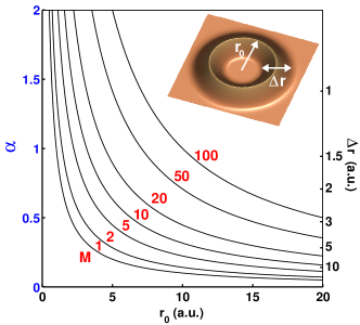
Figure 1: (color online) Relation between the parameter set ($\alpha$, $M$) in the external confining potential [Eq. (4)] and the single-electron ring radius $r_{0}$ and width $\Delta r$ (see the inset). The curves correspond to fixed values of $M$.

we show explicitly the relation between the single-electron radius and width of the QR ($r_{0},\Delta r$) and the parameters ($M,\alpha$) in the external confining potential given in Eq. (4).

The exact exchange-hole function for the single-electron wavefunction in Eq. (5) becomes

$$h^{\sigma}_{x,1}({\bf r}_{1},{\bf r}_{2}) = \psi^{*}_{\sigma}({\bf r}_{2})\psi_{\sigma}({\bf r}_{2})=\rho_{\sigma}({\bf r}_{2})$$ (6)

$$= \frac{\alpha^{2(M+1)}}{\pi M!}\;r_{2}^{2M}\,e^{-\alpha^{2}r_{2}^{2}}.$$

To calculate the cylindrical average as defined in Eq. (3), we first set ${\bf r}_{1}={\bf r}$ and ${\bf r}_{2}={\bf r}+{\bf s}$. As a result we get

$$\bar{h}^{\sigma}_{x,1}({\bf r},s)=\frac{1}{2\pi}\int_{0}^{2\pi}d\phi_{s}\,\rho_{\sigma}({\bf r}+{\bf s})\\ =\frac{\alpha^{2(M+1)}}{\pi M!}e^{-\alpha^{2}(r^{2}+s^{2})}(r^{2}+s^{2})^{M}\\ \times\sum_{k=0}^{M}(-1)^{k}\binom{M}{k}\left(\frac{2rs}{r^{2}+s^{2}}\right)^{k}\frac{d^{k}}{dz^{k}}I_{0}(z){\Big{|}}_{z=2\alpha^{2}rs},$$ (7)

where $I_{0}(z)$ is the zeroth-order modified Bessel function of the first kind, and $M$ is now an integer.

Next, we apply $\bar{h}^{\sigma}_{x,1}$ as a general model for the averaged exchange hole of an $N$-electron system. becke ; expaper The model is required to locally reproduce the short-range behavior of the exchange hole. Therefore, we parametrize $\alpha^{2}$ and $r^{2}$ into functions of $r$ by setting $\alpha^{2}\rightarrow a(r)$ and $r^{2}\rightarrow b(r)$. Equation (7) can be now rewritten as

$$\bar{h}^{\sigma}_{x}(a,b;s)=\frac{a^{M^{*}+1}}{\pi{M^{*}}!}e^{-a(b+s^{2})}(b+s^{2})^{M^{*}}\\ \times\sum_{k=0}^{M^{*}}(-1)^{k}\binom{M^{*}}{k}\left(\frac{2\sqrt{b}s}{b+s^{2}}\right)^{k}\frac{d^{k}}{dz^{k}}I_{0}(z){\Big{|}}_{z=2a\sqrt{b}s}.$$ (8)

where $M^{*}=2(\Delta r^{*}/r^{*}_{0})^{-2}$ is the nearest integer describing the characteristic ratio between the effective width and the radius of the $N$-electron QR. As we will show below, $r_{0}^{*}$ and $\Delta r^{*}$ can be extracted from the spin density. As a consequence, $M^{*}$ can be considered as a (spin) density functional $M^{*}[\rho_{\sigma}]$. The short-range behavior with respect to $s$ can be obtained from the first two non-vanishing terms in the Taylor expansion in Eq. (3):

$$\bar{h}^{\sigma}_{x}({\bf r},s)=\rho_{\sigma}({\bf r})+s^{2}C^{\sigma}_{x}({\bf r})+\ldots,$$ (9)

where

$$C^{\sigma}_{x}=\frac{1}{4}\left[\nabla^{2}\rho_{\sigma}-2\tau_{\sigma}+\frac{1}{2}\frac{\left(\nabla\rho_{\sigma}\right)^{2}}{\rho_{\sigma}}+2\frac{{\bf j}^{2}_{p,\sigma}}{\rho_{\sigma}}\right],$$ (10)

is the local curvature of the exchange hole in 2D expaper around the given reference point ${\bf r}$ (argument omitted). Here the (double of the) kinetic-energy density, $\tau_{\sigma}=\sum_{k=1}^{N_{\sigma}}|\nabla\psi_{k,\sigma}|^{2}$, and the spin-dependent paramagnetic current density, ${\bf j}_{p,\sigma}=\frac{1}{2i}\sum_{k=1}^{N_{\sigma}}\left[\psi^{*}_{k,\sigma}\left(\nabla\psi_{k,\sigma}\right)-\left(\nabla\psi^{*}_{k,\sigma}\right)\psi_{k,\sigma}\right]$, depend explicitly on the KS orbitals, and hence implicitly on the spin densities. Defining $y(r):=a(r)b(r)$, the zeroth-order term in Eq. (9) yields

$$\rho_{\sigma}=\frac{a}{\pi{M^{*}}!}y^{M^{*}}e^{-y},$$ (11)

and the second-order term gives

$$C_{x}^{\sigma}=\frac{a^{2}}{\pi M^{*}!}y^{M^{*}-1}\big{[}(y-M^{*})^{2}-y\big{]}e^{-y}.$$ (12)

Combining Eqs. (11) and (12) leads to

$$M^{*}!\,y^{-(M^{*}+1)}\big{[}(y-M^{*})^{2}-y\big{]}e^{y}=\frac{C_{x}^{\sigma}}{\pi\rho^{2}_{\sigma}},$$ (13)

from which $y$ can be solved numerically. Now, we can compute $a$ and $b$ and thus the averaged exchange hole from Eq. (8). The exchange-hole potential is given by

$$U^{\sigma}_{x}({\bf r})=-2\pi\int_{0}^{\infty}ds\,\bar{h}^{\sigma}_{x}(a,b;s),$$ (14)

from which the exchange energy can be calculated as

$$E_{x}[\rho_{\uparrow},\rho_{\downarrow}]=\frac{1}{2}\sum_{\sigma}\int d{\bf r}\,\rho_{\sigma}({\bf r})U^{\sigma}_{x}({\bf r}).$$ (15)

From Eqs. (8) and (14) it can be shown that our calculation scheme preserves also the exact long-range behavior: $U_{x}^{\sigma}(r\rightarrow\infty)\rightarrow-1/r$. new

To summarize our method, the calculation of the exchange energy of an $N$-electron QR consists of the following steps:

• Use the KS orbitals $\psi_{k,\sigma}$ to calculate the spin densities $\rho_{\sigma}$, the local curvature of the exchange hole $C^{\sigma}_{x}$ from Eq. (10), and to estimate $M^{*}$.

• Compute $y(r)$ numerically from Eq. (13).

• Calculate $a(r)$ from Eq. (11) and $b(r)$ from the relation $b(r)=y(r)/a(r)$.

• Calculate the averaged exchange-hole function from Eq. (8).

• Finally calculate the exchange-hole potential and the exchange energy from Eqs. (14) and (15), respectively.

Next we test the performance of our functional in a few examples. As the reference results we use the exchange-hole potentials and exchange energies of the EXX calculations within the rather accurate Krieger-Li-Iafrate (KLI) approximation. KLI We compare the results also to the 2D-LSDA. Both the EXX and LSDA results are obtained using the octopus code. octopus The converged EXX orbitals are used as the input KS orbitals in our functional (and in the LSDA). Alternatively, also the LSDA orbitals can be used as input, which in most cases leads to only minor changes in the results.

Figure 2

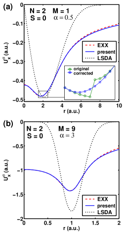
Figure 2: (color online) Exchange-hole potentials of two-electron quantum rings (total spin $S=0$) defined by parameters (a) $M=1$, $\alpha=0.5$, and (b) $M=9$, $\alpha=3$. The dashed line shows the exact-exchange (EXX) result, the solid line is the result of the present work, and the dotted line corresponds to the exchange-energy density in the local spin-density approximation (LSDA).

shows the exchange-hole potentials for two-electron singlet states of two QRs defined by (a) ($M,\alpha$)=($1,0.5$) and (b) ($M,\alpha$)=($9,3$), respectively. Note that here we have set $M^{*}=M$ as the first approximation. In both cases we find excellent agreement between the EXX (dashed lines) and the present work (solid lines). Both the large-$r$ limit, where $U^{\sigma}_{x}$ decays as $-1/r$, and also the $r\rightarrow 0$ limit, are correctly reproduced.

The exchange energies per particle of the LSDA (dotted lines in Fig. 2), which are directly comparable to $U_{x}^{\sigma}$, deviate significantly from the EXX and from our approximation. The inability of the LSDA to yield the correct shape of the curve is due to the simple density-dependent expression of the exchange energy per particle in the LSDA, i.e., $\epsilon^{\rm LSDA}_{x,\sigma}\propto\rho_{\sigma}^{1/2}$, leading to differences also in the exchange energy. In the case of Fig. 2(a), we find $E^{\rm LSDA}_{x}=-0.389$, whereas $E^{\rm EXX}_{x}=-0.409$ and $E^{\rm present}_{x}=-0.408$. When the ratio $\Delta r/r_{0}$ is decreased to one third, i.e., $M=1\rightarrow 9$, the deviation of the LSDA becomes more pronounced as shown in Fig. 2(b). Now we find $E^{\rm LSDA}_{x}=-1.502$ vs. $E^{\rm EXX}_{x}=E^{\rm present}_{x}=-1.300$. In other words, the above change in $M$ increases the relative error of the LSDA exchange energy from $5\%$ to $16\%$. Hence, these results demonstrate the breakdown of the 2D-LSDA in the quasi-one-dimensional limit.

At this point we make two remarks of the numerical procedure. First, Eq. (13) has two solutions for $y(r)$, from which we choose the smaller one for $r<r[\rho_{\rm max}]$ and the larger one otherwise. Since these two solutions do not generally coincide at $r=r[\rho_{\rm max}]$, we extrapolate $U_{x}^{\sigma}(r)$ around this point as visualized in the inset of Fig. 2. This smoothing procedure is done such that $E_{x}$ is not altered. Second, the application of the overall scheme might be numerically cumbersome in the small-$r$ regime when $M$ (and/or $M^{*}$) is large and the density is very small. To overcome this problem, we take the advantage of the exact property of our model, $U_{x}^{\sigma}(r\rightarrow 0)=-(2M)!\,(M!)^{-2}\,2^{-2M}\,\alpha\sqrt{\pi}+O(r^{2})$, which is valid for a general $N$-electron case with $M>1$. new

To demonstrate the generality of our method, we show in Fig. 3

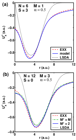
Figure 3: (color online) Same as in Fig. 2 but for (a) a fully spin-polarized current-carrying six-electron quantum ring at $B=6$ T and for (b) a zero-current 12-electron quantum ring.

the exchange-hole potentials for (a) a spin-polarized current-carrying six-electron QR at $B=6$ T and for (b) a 12-electron QR. Similarly to the previous examples, we find excellent agreement with the EXX. The six-electron case yields $E^{\rm EXX}_{x}=-2.226$, $E^{\rm present}_{x}=-2.238$, and $E^{\rm LSDA}_{x}=-2.114$. In the case of 12 electrons, we plot results for both $M^{*}=M=3$ and for $M^{*}[\rho]=2\approx 2(\Delta r^{*}/r^{*}_{0})^{-2}$, where the effective radius $r^{*}_{0}$ corresponds to the point where the cumulative density reaches $50\,\%$, and the effective width $\Delta r^{*}$, centered at $r^{*}_{0}$, covers $90\,\%$ of the total density. We find that in the latter case the agreement with the EXX is better.

To conclude, we have derived, from first principles, an accurate and general approximation for the exchange-hole potential and hence for the exchange energy in quantum rings. Excellent agreement with the exact-exchange results is obtained regardless of the ring geometry, number of electrons, spin polarization, and currents. Moreover, we have demonstrated that, in contrast to the local-density approximation, our functional can deal with the physically relevant dimensional crossover between two and one dimensions. Our approach is suitable for the development of correlation functionals by considering the exact properties of the corresponding correlation-hole potentials. corr_paper

- (1) A. Lorke, R. J. Luyken, A. O. Govorov, J. P. Kotthaus, J. M. Garcia, and P. M. Petroff, Phys. Rev. Lett. 84, 2223 (2000).
- (2) A. Fuhrer, S. Lüscher, T. Ihn, T. Heinzel, K. Ensslin, W. Wegscheider, and M. Bichler, Nature (London) 413, 822 (2001).
- (3) U. F. Keyser, C. Fühner, S. Borck, R. J. Haug, M. Bichler, G. Abstreiter, and W. Wegscheider, Phys. Rev. Lett. 90, 196601 (2003).
- (4) Y. Aharonov and D. Bohm, Phys. Rev. 115, 485 (1959).
- (5) See, e.g., M. Sigrist, A. Fuhrer, T. Ihn, K. Ensslin, S. E. Ulloa, W. Wegscheider, and M. Bichler, Phys. Rev. Lett. 93, 066802 (2004).
- (6) E. Räsänen, A. Castro, J. Werschnik, A. Rubio, and E. K. U. Gross, Phys. Rev. Lett. 98, 157404 (2007).
- (7) S. Viefers, P. Koskinen, P. Singha Deo, and M. Manninen, Physica E (Amsterdam) 21, 1 (2004).
- (8) M. M. Fogler and E. Pivovarov, Phys. Rev. B 72, 195344 (2005).
- (9) K. Niemelä, P. Pietiläinen, P. Hyvönen, and T. Chakraborty, Europhys. Lett. 36, 533 (1996).
- (10) S. S. Gylfadottir, A. Harju, T. Jouttenus, C. Webb, New J. of Physics 8, 211 (2006).
- (11) A. Emperador, F. Pederiva, and E. Lipparini, Phys. Rev. B 68, 115312 (2003).
- (12) A. Emperador, M. Pi, M. Barranco, and E. Lipparini, Phys. Rev. B 64, 155304 (2001).
- (13) M. Aichinger, S. A. Chin, E. Krotscheck, and E. Räsänen, Phys. Rev. B 73, 195310 (2006).
- (14) E. Räsänen and M. Aichinger, J. Phys.: Cond. Matt. 21, 025301 (2009).
- (15) C. Attaccalite, S. Moroni, P. Gori-Giorgi, and G. B. Bachelet, Phys. Rev. Lett. 88, 256601 (2002).
- (16) For a review, see, e.g., L. P. Kouwenhoven, D. G. Austing, and S. Tarucha, Rep. Prog. Phys. 64, 701 (2001); S. M. Reimann and M. Manninen, Rev. Mod. Phys. 74, 1283 (2002).
- (17) Y.-H. Kim, I.-H. Lee, S. Nagaraja, J.-P. Leburton, R. Q. Hood, and R. M. Martin, Phys. Rev. B 61, 5202 (2000); L. Pollack and J. P. Perdew, J. Phys.: Condens. Matter 12, 1239 (2000).
- (18) N. Helbig, S. Kurth, S. Pittalis, E. Räsänen, and E. K. U. Gross, Phys. Rev. B 77, 245106 (2008).
- (19) See, e.g., T. Heaton-Burgess, F. A. Bulat, and W. Yang, Phys. Rev. Lett. 98, 256401 (2007); V. N. Staroverov and G. E. Scuseria, J. Chem. Phys. 124, 141103 (2006); ibid 125, 081104 (2006); D. R. Rohr, O. V. Gritsenko, and E. J. Baerends, J. Mol. Structure: THEOCHEM 72, 762 (2006); A. Hesselmann, A. W. Götz, F. Della Sala, and A. Görling, J. Chem. Phys. 127, 054102 (2007).
- (20) S. Pittalis, E. Räsänen, C. Proetto, and E. K. U. Gross, Phys. Rev. B (in print).
- (21) A. D. Becke and M. R. Roussel, Phys. Rev. A 39, 3761 (1989).
- (22) S. Pittalis, E. Räsänen, N. Helbig, and E. K. U. Gross, Phys. Rev. B 76, 235314 (2007).
- (23) W.-C. Tan and J. Inkson, Semicond. Sci. Technol. 11, 1635 (1996).
- (24) S. Pittalis et al. (unpublished).
- (25) J. B. Krieger, Y. Li, and G. J. Iafrate, Phys. Rev. A 46, 5453 (1992).
- (26) A. K. Rajagopal and J. C. Kimball, Phys. Rev. B 15, 2819 (1977).
- (27) A. Castro, H. Appel, M. Oliveira, C. A. Rozzi, X. Andrade, F. Lorenzen, M. A. L. Marques, E. K. U. Gross, and A. Rubio, Phys. Stat. Sol. (b) 243, 2465 (2006).