Large temperature dependence of the Casimir force at the metal-insulator transition

Abstract

The dependence of the Casimir force on material properties is important for both future applications and to gain further insight on its fundamental aspects. Here we derive a general theory of the Casimir force for low-conducting compounds, or poor metals. For distances in the micrometer range, a large variety of such materials is described by universal equations containing a few parameters: the effective plasma frequency $\omega_{p}$, dissipation rate $\gamma$ of the free carriers, and electric permittivity $\varepsilon_{\infty}$ for $\omega\geq\omega_{p}$ (in the infrared range). This theory can also describe inhomogeneous composite materials containing small regions with different conductivity. The Casimir force for mechanical systems involving samples made with compounds that have a metal-insulator transition shows an abrupt large temperature dependence of the Casimir force within the transition region, where metallic and dielectric phases coexist.

I Introduction and motivation

The Casimir force 1 has demonstrated the reality of zero-point field fluctuations, which played a significant role in the development of quantum field theory (see, e.g., the monographs m1 ; m3 and review papers r1 ; 5 ; r3 ; PhysicsToday ). The Casimir effect attracts considerable attention because of its numerous applications in quantum field theory, atomic physics, condensed matter physics, gravitation and cosmology. m1 ; m3 ; r1 ; 5 ; r3 ; PhysicsToday ; f ; BECPit ; 9 The experimental observation of the Casimir force is of fundamental importance. Despite the fact that the magnitude of the Casimir force is quite small, its presence is established by a number of experiments, usually done for metallic samples; see, e.g., Refs. 9, ; exp1, ; 10, ; 11, ; 12, ; exp2, . Furthermore, this force is relevant for various nanomechanical devices, where the space separation of nearby plates is very small. 8 ; m3 ; r3

I.1 Casimir force for good metals and dielectrics

The Casimir force between two macroscopic samples is caused by a spatial redistribution of the fluctuations of the electromagnetic field compared to that of free space because of the presence of the samples. For the simplest case of two parallel perfectly conducting thick metallic plates placed in vacuum and separated by a distance $l$, the Casimir force per unit area of the sample at zero temperature can be written as

$$F_{\mathrm{C}}=\frac{\pi^{2}}{240}\frac{c\hbar}{l^{4}},$$ (1)

where $c$ is the speed of light, and $\hbar$ is the Planck constant. For dielectric bodies with frequency-dependent dielectric permittivities, the value of this force has been found by Lifshitz.2 If the permittivity $\varepsilon$ is frequency-independent, for two equivalent dielectric bodies or for a dielectric sample and an ideal metal, this force can be written as

$$F_{\mathrm{L}}=\frac{\pi^{2}}{240}\frac{c\hbar}{l^{4}}\cdot\left({\frac{\varepsilon-1}{\varepsilon+1}}\right)^{\nu}\varphi_{\nu}(\varepsilon),$$ (2)

where $\nu=2$ for two equivalent dielectric bodies and $\nu=1$ for the interaction of a dielectric sample and a metal. The function $\varphi_{\nu}(\varepsilon)\to 1$ when $\varepsilon\gg 1$, and $\varphi_{\nu}(\varepsilon)$ decreases when $\varepsilon\to 1$; in particular, $\varphi_{1}(\varepsilon\to 1)=0.46$ and $\varphi_{2}(\varepsilon\to 1)=0.35$. Strictly speaking, equations of type (1) or (2) are valid when $l<\hbar c/kT$, where only the zero-point fluctuations of the electromagnetic field are important (see Refs. 3, ; 4, ; 5, for details). At room temperature, this inequality is valid for distances less then a few micrometers. Below we will only consider this range.

I.2 Material aspects of the Casimir force

To study the Casimir force, different materials can be used. Indeed, it is important to understand how this force is affected by the choice of different materials. For example, recent studies, using silicon with different degrees of doping semicond ; Exper07 or materials for sensors, like Vanadium oxide Exper07 , have shown numerous specific features which are absent in the good metals traditionally used to study the Casimir force.

The investigation of material-dependent features of the Casimir force is important not only for future applications, but also for fundamental physics. To discuss the material-dependent aspects of the Casimir force, let us note the following. The well-known results present in the expressions (1) and (2) are obtained for frequency-independent values of the electrical permittivity $\varepsilon$. For metals, this means $\varepsilon=\infty$ for any frequency. Detailed investigations, taking into account the dispersion of the media, have shown 3 ; 4 that the universal formula of the type $F_{\mathrm{C}}\propto 1/l^{4}$ is valid for distances $l>\lambda_{0}$, where $\lambda_{0}=c/\omega_{0}$, and $\omega_{0}$ is the highest characteristic frequency of the media. Beyond this approximation, the Casimir force $F$ can be written 2 ; 3 ; 4 ; 5 as

$$F=\frac{\hbar}{2\pi^{2}c^{3}}\cdot\int\limits_{0}^{\infty}{\zeta^{3}d\zeta}\cdot\Phi[\varepsilon(i\zeta)],$$ (3)

where $\varepsilon=\varepsilon(i\zeta)$ is the complex permittivity of the media, the summation over the Matsubara frequencies is replaced by integration over $\zeta$ (this is adequate 3 when $l<\hbar c/kT$), $\Phi[\varepsilon(i\zeta)]$ is a functional of the function $\varepsilon(i\zeta)$,

$$\Phi[\varepsilon(i\zeta)] = \int\limits_{1}^{\infty}{p^{2}dp\biggl{(}\frac{1}{A_{1}^{\nu}e^{x}-1}}+\frac{1}{A_{2}^{\nu}e^{x}-1}\biggl{)},$$ (4)

$$A_{1} = \frac{s+p}{s-p},\quad A_{2}=\frac{p\varepsilon+s}{p\varepsilon-s},\quad s=\sqrt{\varepsilon+p^{2}-1}\;,$$

where $x=2p\zeta l/c$. Two terms in Eq. (4) describe the contributions of the modes with two different polarizations of the electric field, parallel to the surface and parallel to the incidence plane (which includes the normal to the surface and the wave vector of the photon), respectively. The exponents $\nu=2$ and $\nu=1$ correspond to the same cases as for Eq. (2), namely, the interaction between two equivalent dispersive media ($\nu=2$), and dispersive medium, interacting with an ideal metal ($\nu=1$). The general properties of the function $\varepsilon(i\zeta)$ are the following: $\varepsilon(i\zeta)$ is a monotonic function of $\zeta$, and $\varepsilon(\zeta)\to 1$ for the values of $\zeta$ higher than all the characteristic frequencies $\zeta>\omega_{0}$ of the medium. For metals, the plasma frequency $\omega_{\mathrm{p}}$ is the highest frequency $\omega_{0}$. Thus, the standard Casimir result (1) is valid for large distances $l>\lambda_{p}=c/\omega_{p}$ between the plates, see Ref. 3, . For the opposite limit case3 of smaller distances, $l<\lambda_{p}$,

$$F(l\to 0)=\frac{\hbar}{8\pi^{2}l^{3}}\bar{\omega},\quad\bar{\omega}=\int\limits_{0}^{\infty}{\left(\frac{\varepsilon-1}{\varepsilon+1}\right)^{\nu}d\zeta}\;,$$ (5)

where the real dispersion, e.g., the dependence of the media permittivity on the frequency, is used.

I.3 Caviats and limitations

It is worth noting here that, as far as we know, only one experiment 10 has been performed using the parallel-plate configuration originally envisioned by Casimir. Most measurements of the Casimir force have studied the interaction of a spherical probe with a flat substrate, using the so-called Proximity Force Theorem PrT to relate the force for different geometries of the experiment to the force between two parallel plates. The experimental search for corrections to this approximation has been done recently. PFTcorr For the original plane-parallel geometry, the accuracy of the measurements 10 of the Casimir force, done for distances ranging from 0.5 to 6 micrometers, is not very high, within 15%. A significant difficulty has been the necessity to keep the samples parallel during the measurements at different distances. Some of these problems, in principle, could be overcome by measuring the Casimir force in a fixed geometry of the experiment (fixed $l$, for plane-parallel geometry) by varying some parameters of the sample. The media properties could be changed by varying the temperature of the sample. Varying the carrier density of semiconductors by laser irradiation has also been proposed recently. semicond ; Exper07

The Casimir force for standard metals has a weak temperature dependence. For metals, the Drude formula, $\varepsilon=1+\omega_{p}^{2}/\zeta(\zeta+\gamma)$ is typically used, where $\omega_{p}$ is the metal plasma frequency and $\gamma$ is the relaxation rate. For typical metals like copper, aluminum or gold, the plasma frequency is practically temperature-independent, and the only way to modify the Casimir force by changing the metal parameters is via the temperature dependence of $\gamma$. For such metals, $\gamma\ll\omega_{p}$, and the corresponding corrections are small. Another problem: for standard metals the value of $\lambda_{p}=c/\omega_{p}$ lies in the ultraviolet region, $\lambda_{p}\leq 0.1\ \mu$m. Thus, to observe dispersive effects, the region $l\leq\lambda_{\mathrm{p}}$ should be investigated, which is quite difficult experimentally. 12 This limitation can be overcome by using thin metallic films,13 but even for this optimal case the temperature corrections are not higher than a few percent.

I.4 Casimir force for pure metals and compounds

Numerous compounds are known for which the carrier density and plasma frequency $\omega_{p}$ are abnormally small. The investigation of such conducting systems, which can be called “poor metals”, is of interest from the point of view of both fundamental physics and applications. Examples include highly doped silicon semicond ; Exper07 , left-handed materials left , transition metal oxides showing the metal-insulator transition (MIT) MIT , cuprate high-temperature superconductors HTCS , and manganites where the phenomenon of colossal magnetoresistance is observed. CMR For all of these systems, both the free carrier density and the plasma frequency $\omega_{p}$ are much smaller than for standard good metals. This means, that in contrast to the usual metals, $\omega_{p}$ is not the highest frequency of the material. The Drude behavior is observed up to infrared frequencies, but with a relatively large value of $\varepsilon=\varepsilon_{\infty}$ when $\omega\gg\omega_{p}$; this value, $\varepsilon_{\infty}\cong 5$–$10$, is determined by transitions of electrons in occupied bands. Thus, $\varepsilon\neq 1$ within a wide frequency region, including the “metallic region”, from small $\omega$ up to a few $\omega_{p}$. The dissipation rate $\gamma$ for poor metals can be quite high, of the order of a few percent, or even a few tenths of $\omega_{p}$. The manifestation of the dispersion for the frequencies corresponding to distances of the order of a few microns provides the possibility to control the Casimir force by varying the parameters of the metal. Recently, measurements of the Casimir force between a metallic sphere and a sample made with a low-conduction medium, like silicon with different degrees of doping and vanadium dioxide VO₂, were proposed Exper07 for small separations, around 200–400 nm.

Here we develop a general theory of the Casimir force for low-conducting compounds, i.e., poor metals. We show that, for distances in the sub-micrometer and micrometer ranges, the Casimir force for a large variety of such systems can be described by formulae that depend on a small number of parameters, without details of the total spectral characteristics. The inhomogeneous composite systems considered here, containing small regions of different properties, can be described within this theory. The application of these results to the region of the metal-insulator transition, where the metallic and dielectric phases coexist, produces a very pronounced temperature dependence of the Casimir force.

II Derivation of the Casimir force for poor metals

For general dispersive media, the Casimir force is determined by the integral in Eq. (4). Keeping in mind the large variety of poor-metal parameters discussed above, we now need to develop an analytical approach to estimate the integral (4) and to study the role of different parameters, like $\epsilon_{\infty}$ or $\gamma/\omega_{p}$, describing the system. Let us now use a two-scale model for $\varepsilon(\zeta)$ as follows:

$$\varepsilon=E(\zeta)\left[1+\frac{\omega_{\mathrm{p}}^{2}}{\zeta(\zeta+\gamma)}\right],$$ (6)

where the function $E(\zeta)$ describes the high frequency dependence of $\varepsilon$. As we will show below, the detailed properties of this function are not important in the region of interest: $l\sim 1$ $\mu$m. The function $E(\zeta)$ is almost constant, $E(\zeta)=\varepsilon_{\infty}$, for all the metallic region, $\omega_{\mathrm{p}}\sim\omega\ll\omega_{0}$, and tends to one for $\omega\gg\omega_{0}$. Obviously, for such a model the standard Casimir behavior in Eq. (1) is valid at large enough distances: $l\gg\lambda_{p}\sim 1\ \mu$m.

To calculate the Casimir force for distances of the order of $c/\omega_{\mathrm{p}}\sim 1$ $\mu$m we use the general equation (3) rewritten as

$$F=\frac{\hbar}{2\pi^{2}c^{3}}\left[\int\limits_{0}^{\left\langle\omega\right\rangle}\zeta^{3}d\zeta\Phi\left[\varepsilon_{\infty}\cdot\left(1+\frac{\omega_{\mathrm{p}}^{2}}{\zeta(\zeta+\gamma)}\right)\right]\right.$$

$$\left.+\int\limits_{\left\langle\omega\right\rangle}^{\infty}{\zeta^{3}d\zeta\Phi[E(\zeta)]}\right].$$

Here the value $\left\langle\omega\right\rangle$ is chosen in the intermediate region:

$$\omega_{p}\ll\left\langle\omega\right\rangle\ll\omega_{0}.$$

Therefore, we replaced $E(\zeta)$ by $\varepsilon_{\infty}$ in Eq. (6) for the first integral and omitted the Drude multiplier for the second integral.

Expanding the integration region over $\zeta$ in both integrals up to $0\leq\zeta<\infty$, and subtracting the extra terms, we present the Casimir force in the form,

$$F=F^{(m)}+\Delta F,$$ (7)

with

$$F^{(m)}=\frac{\hbar}{2\pi^{2}c^{3}}\int\limits_{0}^{\infty}{\zeta^{3}d\zeta\Phi\left[\varepsilon_{\infty}\left(1+\frac{\omega_{p}^{2}}{\zeta(\zeta+\gamma)}\right)\right]},$$ (8)

$$\Delta F=\frac{\hbar}{2\pi^{2}c^{3}}\int\limits_{0}^{\infty}{\zeta^{3}d\zeta\biggl{[}\Phi\left[E(\zeta)\right]-\Phi[\varepsilon_{\infty}]\biggr{]}}.$$ (9)

In the frequency region, $\omega\sim c/l$, which is an important regime for $\Phi[\varepsilon(\zeta)]$, the functions $\Phi[E(\zeta)]$ and $\Phi[\varepsilon_{\infty}]$ in Eq. (9) almost cancel each other. Therefore, the term $\Delta F$ is relatively small. A more detailed analysis gives

$$\Delta F\,\cong\,\frac{\hbar c\lambda_{0}^{2}}{l^{6}}\,\ll\,F.$$

Thus, in the region of interest, $\lambda_{0}\ll l\sim\lambda_{p}$, the Casimir force is described by the first term in Eq. (7), $F=F^{(m)}$.

Now we introduce the variable $z=\zeta l/c$ and write the main contribution to the Casimir force as

$$F=\frac{\pi^{2}}{240}\frac{c\hbar}{l^{4}}\cdot\Pi\equiv F_{\mathrm{C}}\cdot\Pi\;,$$ (10)

where $F_{\mathrm{C}}$ is the Casimir force (1) for ideal metals, the prefactor $\Pi$ depends only on the dimensionless parameters $\tilde{l}=l/\lambda_{p}$, $\varepsilon_{\infty}$, and $\alpha=\gamma/\omega_{p}$,

$$\Pi=\frac{120}{\pi^{4}}\int\limits_{0}^{\infty}{z^{3}}dz\int\limits_{1}^{\infty}p^{2}dp$$

$$\times\left[\frac{1}{A_{1}^{\nu}\exp(x)-1}+\frac{1}{A_{2}^{\nu}\exp(x)-1}\right],$$ (11)

where $A_{1}$ and $A_{2}$ are given by Eq. (4) with

$$\varepsilon=\varepsilon_{\infty}\left[1+\frac{\tilde{l}^{2}}{z(z+\alpha\tilde{l})}\right].$$

II.1 Computing the Casimir force integrals

To proceed further, let us change the variable $z$ by $x=z/2p$ in Eq. (11), and note, that the integral $\int\limits_{0}^{\infty}{(Ae^{x}-1)^{-1}x^{3}dx}$, with $A=A(x,p)$ being a smooth function of $x$, can be approximated by $1/A(x_{0},p)$ with $x_{0}\sim 4$. The problem is then reduced to calculating two one-dimensional integrals, $J_{1}$ and $J_{2}$:

$$J_{1,2}=\int\limits_{1}^{\infty}{\frac{dp}{p^{2}}}\frac{1}{A_{1,2}},\quad\Pi=\frac{1}{2}(J_{1}+J_{2}),$$ (12)

where $A_{1}$ and $A_{2}$ are given by Eq. (4) with the substitution

$$\varepsilon=\varepsilon_{\infty}\left[1+\frac{4\tilde{l}^{2}p^{2}}{x_{0}(x_{0}+2p\alpha\tilde{l})}\right].$$ (13)

The validity of this approximation is confirmed by the numerical calculation of integral (11), as shown in Fig. 1. The function $\Pi(\tilde{l})$ found numerically is shown in Fig. 2. A simple analysis of Eq. (12) gives us two limit cases.

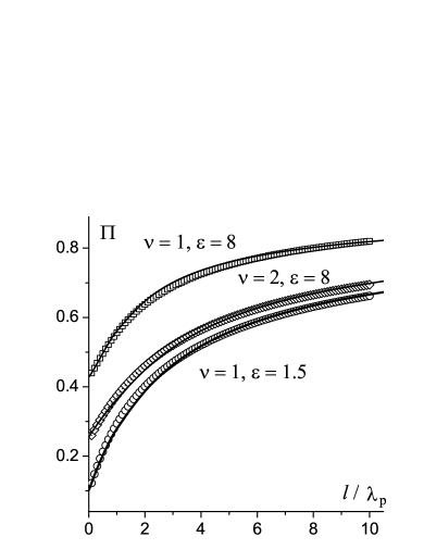
Figure 1: The normalized Casimir force $\Pi=F/F_{\mathrm{C}}$ versus $l/\lambda_{p}$ for some values of parameters (shown near curves). This plot compares the results of numerical calculations of the two-dimensional integral Eq. (11) for the prefactor $\Pi$ (symbols) with the results within the approximate approach based on Eq. (12) (solid curves). This plot shows a very good agreement between both.

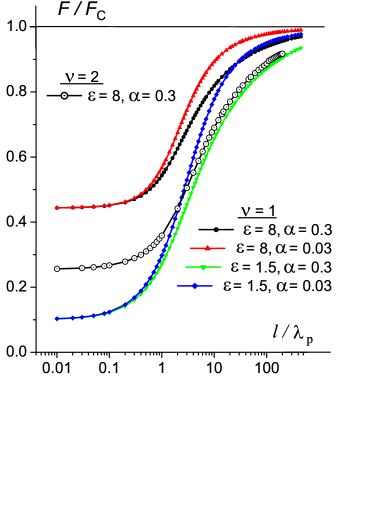
Figure 2: (Color online) The normalized Casimir force $\Pi=F/F_{\mathrm{C}}$ versus the parameter $\tilde{l}=l/\lambda_{p}$, for $\nu=1,2$, using the typical value $\varepsilon_{\infty}=8$, as well as the smaller $\varepsilon_{\infty}=1.5$, and different values of the dissipation parameter $\alpha=\gamma/\omega_{p}$. The horizontal line on top gives the asymptotic value $F/F_{\mathrm{C}}=\Pi=1$ for an ideal metal.

For small $\tilde{l}\leq 0.3$ the value of $\alpha$ plays a minor role. In this region, the value of $\Pi$ practically does not depend on $\tilde{l}$ and reproduces well the Lifshitz’s result (2) for dielectric media with a $\zeta$-independent $\varepsilon=\varepsilon_{\infty}$ and $\gamma=0$,

$$\Pi_{\mathrm{L}}\equiv\left(\frac{\varepsilon_{\infty}-1}{\varepsilon_{\infty}+1}\right)^{\nu}\cdot\varphi_{\nu}(\varepsilon_{\infty}).$$

We now emphasize that the dependence of the Casimir force, proportional to $\bar{\omega}/l^{3}$, see Eq. (5), is not realized for any $\varepsilon_{\infty}\neq 1$.

Otherwise, in the limit case $\tilde{l}\to\infty$, the integrals $J_{1}=J_{2}=1$, and the ideal Casimir limit (1) is recovered. In contrast to the case of small values of $\tilde{l}$, the dependence of $\Pi$ on $l$ for large, but finite values of $\tilde{l}$ shows an interesting and unexpected behavior: the approach to saturation is quite slow, especially for large values of

$$\alpha=\frac{\gamma}{\omega_{p}}\,.$$

In other words, it is hard to reach the metallic limit value of $\Pi=1$ when $\alpha>0.1$, for the most interesting region $\tilde{l}\leq 10$.

To understand this behavior, let us now investigate in more details the factor $\Pi$ for not so small values of $\tilde{l}$. As has been mentioned above, it is a sum of two contributions from the electromagnetic fields of different polarizations. It is convenient to examine the first and second integrals separately. Numerical calculations show that the behavior of these two integrals, $J_{1}$ and $J_{2}$, is essentially different for the same values of parameters, as shown in Fig. 3.

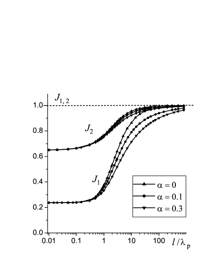
Figure 3: Integrals $J_{1}$ and $J_{2}$, defined by Eq. (12), describing the Casimir force versus $l/\lambda_{p}$ for $\varepsilon_{\infty}=8$ and different values of the dissipation parameter $\alpha=\gamma/\omega_{p}$ (shown in the figure). Symbols depict the results of numerical calculations.

The two interesting features (i.e., the slow approach to saturation and the essential dependence of $\Pi$ on $\alpha=\gamma/\omega_{p}$) are mostly associated with the first integral, $J_{1}$, which describes the contribution of the fluctuations with the electric field parallel to the surfaces of plane-parallel samples. This integral $J_{1}$ can be calculated analytically. For $\alpha=0$, it can be written as

$$J_{1}=1-\frac{2}{b}\cdot\ln\left(\frac{\sqrt{a^{2}+b^{2}}+b}{a}\right)+\\ +\frac{4}{b\sqrt{a^{2}-1}}\cdot\arctan\left(\frac{\sqrt{a^{2}-1}}{a+1}\cdot\frac{\sqrt{a^{2}+b^{2}}+b-a}{\sqrt{a^{2}+b^{2}}+b+a}\right)\;,$$ (14)

where we introduce the notation

$$a^{2}=1+\varepsilon_{\infty}\frac{\tilde{l}^{2}}{4},\quad b^{2}=\varepsilon_{\infty}-1.$$

For non-zero dissipation rate, $\alpha\neq 0$, the analytical formula for $J_{1}$ is very long and inconvenient for real estimates. But for the case of interest, $\tilde{l}\geq 3$, the integral $J_{1}$ can be well approximated with the simpler expression

$$J_{1,\,\mathrm{appr}}=\frac{\sqrt{(3+\varepsilon_{\infty})(3+5\alpha\tilde{l})+3\varepsilon_{\infty}\tilde{l}^{2}}-2\sqrt{3+5\alpha\tilde{l}}}{\sqrt{(3+\varepsilon_{\infty})(3+5\alpha\tilde{l})+3\varepsilon_{\infty}\tilde{l}^{2}}+2\sqrt{3+5\alpha\tilde{l}}}\;,$$ (15)

as shown in Fig. 4

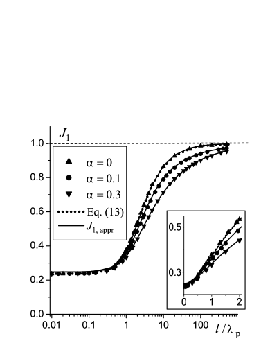
Figure 4: The integral $J_{1}$ versus $l/\lambda_{p}$ for $\varepsilon_{\infty}=8$ and different values of the dissipation parameter $\alpha=\gamma/\omega_{p}$. Symbols depict the results of numerical calculations. The detailed behavior of $J_{1}$ for small $\tilde{l}$ is present in the inset. The dotted line describes the analytical result Eq. (14) for $\alpha=0$, solid lines are drawn in accordance with the approximate formula Eq. (15).

This equation explains the complicated behavior of the factor $\Pi=F/F_{\mathrm{C}}$ for large $\tilde{l}$, and especially, the role of the dissipation constant $\alpha$. For any finite value of $\alpha$ and extremely large $\tilde{l}$, $\tilde{l}\gg 1$ and $\tilde{l}\gg 1/\alpha$, $J_{1}$ versus $\tilde{l}$ has a very slow inverse-square-root dependence,

$$J_{1}\simeq 1-\frac{4\sqrt{5\alpha}}{\sqrt{3\varepsilon_{\infty}}}\cdot\frac{1}{\sqrt{\tilde{l}}},\quad\tilde{l}\gg 1,\,1/\alpha.$$ (16)

For very small $\alpha\ll 1$, the intermediate region $1/\alpha\gg\tilde{l}\gg 1$ appears. For this region, the behavior of $J_{1}$ is sharper,

$$J_{1}\simeq 1-\frac{2}{\sqrt{\varepsilon_{\infty}}}\cdot\frac{1}{\tilde{l}}\,,\quad 1/\alpha\gg\tilde{l}\gg 1\;.$$ (17)

An analytical expression for $J_{2}$ in terms of elementary functions cannot be written. Fortunately, the integral $J_{2}$ exhibits a simpler behavior than $J_{1}$, and for its description we can use a simple approximation. First note the quite weak dependence of the shape of the function $J_{2}(\tilde{l})$ on the value of $\alpha$, as shown in Fig. 5. For the regime of interest here, $\varepsilon_{\infty}\gg 1$, the difference between the values of $J_{2}$ for $\alpha=0.3$ and $\alpha=0$ is maximum near the range $\tilde{l}\sim$ (10–15), and does not exceed 3%. Indeed, all the curves with $0\leq\alpha<0.3$ merge together, and for describing of $J_{2}$ within an accuracy of 1.5%, the function $J_{2}(\tilde{l})$ found for $\alpha=0.1$ can be used. Even for small $\varepsilon_{\infty}=1.5$, the inaccuracy of this approximation is less than 5%.

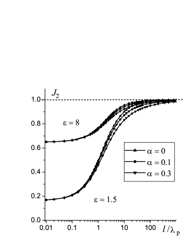
Figure 5: The integral $J_{2}$ calculated numerically for $\varepsilon_{\infty}=8$ and $\varepsilon_{\infty}=1.5$ and different values of $\alpha$ (symbols). The shapes of the curves depend very weakly on $\alpha$.

Numerical data are well fitted by the very simple formula

$$J_{2,\,\mathrm{fit}}=\frac{J_{2,\,\mathrm{L}}+\eta\,\tilde{l}}{1+\eta\,\tilde{l}}\;,$$ (18)

where $\eta\simeq$ (0.5–0.6), $J_{2,\,\mathrm{L}}$ determines the value of $J_{2}$ for small $\tilde{l}\ll 1$, as shown in Fig. 6. The quantity $J_{2,\,\mathrm{L}}$ describes the contribution of $J_{2}$ to the Lifshitz’s result (2) for dielectric media with $\varepsilon=\varepsilon_{\infty}$ and $\alpha=0$.

Figure 6: The integral $J_{2}$ calculated numerically for $\alpha=0.1$ and very different values of the dielectric permittivity, $\varepsilon_{\infty}=8$ and $\varepsilon_{\infty}=1.5$ (symbols). The curves describe the approximating function Eq. (18). Note the very good agreement between numerical data and approximating functions.

Thus, we can present a simple description of the second integral $J_{2}$: it is practically independent on the dissipation parameter $\alpha$, and the dependence on $\varepsilon_{\infty}$ is governed only by the Lifshitz contribution $J_{2,\,\mathrm{L}}$. The asymptotic behavior of $J_{2}$ at large distances $\tilde{l}\gg 1$ is of the form $1-(1-J_{2,\,\mathrm{L}})/\eta\tilde{l}$, which is much weaker than the inverse-square-root dependence (16) for $J_{1}$. For large $\varepsilon_{\infty}\gg 1$, when $(1-J_{2,\,\mathrm{L}})\propto 1/\varepsilon_{\infty}\ll 1$, the dependence $J_{2}(\tilde{l})$ is especially weak, even compared with that for $J_{1}$ in the intermediate region (17).

II.2 Change in the Casimir force near the metal-insulator transition

The analytical formulae derived above give a good description of the behavior of the Casimir force when the metal-insulator transition occurs. Usually, the metal-insulator transition is associated with an abrupt change, by a few orders of magnitude, of the conductivity at a transition temperature $T=T_{c}$. Let us start with a rough picture, assuming that a metallic phase has a finite value of the plasma frequency whereas for the dielectric phase the plasma frequency is zero. Using the results obtained above, one can expect a drastic change of the Casimir force between two plane-parallel samples caused by the change of the parameter $\lambda_{\mathrm{p}}$, very near the metal-insulator transition.

We stress that the change of the force is not connected with changing the physical distance $l$, but with changing the dimensionless quantity $\tilde{l}=l/\lambda_{p}$, caused by the change of the plasma wavelength $\lambda_{\mathrm{p}}=c/\omega_{p}$. Thus, one can expect a jump-like behavior of the Casimir force when changing the temperature across $T_{c}$. Within the transition region, the force changes from the “metallic” value $F^{>}$, typical for finite values of $\tilde{l}$, to the very different value $F^{<}$, for an insulator when $\tilde{l}\ll 1$.

The important quantity here is the change of the Casimir force, $\Delta F=(F^{>}-F^{<})$. To estimate $F^{<}$, we can use the Lifshitz formula (2) valid in the limit $l\ll\lambda_{p}$, which corresponds to the dielectric phase. The value of $F^{>}$ in the metallic phase corresponds to large, but finite values of $l/\lambda_{p}$. To estimate $F^{>}$, note that the dependence of $\Pi$ on $l$ at $10\gtrsim l/\lambda_{p}\gtrsim 2.5$ is mainly provided by the integral $J_{1}$, whereas $J_{2}$ can be replaced by one. Thus, the concrete value of the coefficient $\eta$ in Eq. (18) is not important. Combining all these data together, and restoring the initial parameters of the media, $\omega_{p}$ and $\gamma$, we arrive at the simple estimate,

$$\Delta F=\frac{\pi^{2}}{240}\frac{c\hbar}{l^{4}}\cdot\left[1-\left({\frac{\varepsilon_{\infty}-1}{\varepsilon_{\infty}+1}}\right)\varphi_{1}(\varepsilon_{\infty})-\frac{2}{\omega_{p}}\sqrt{\frac{5c\gamma}{3\varepsilon_{\infty}l}}\right],$$ (19)

where the function $\varphi_{1}(\varepsilon)$ describes the Lifshitz’s result for the interaction of a dielectric sample and an ideal metal. When the value of $\gamma$ is small enough, as for manganites, for the distance $l$ such that $l\ll c/\gamma$, Eq. (17) is valid, and the formula for $\Delta F$ reads

$$\Delta F=\frac{\pi^{2}}{240}\frac{c\hbar}{l^{4}}\cdot\left[1-\left({\frac{\varepsilon_{\infty}-1}{\varepsilon_{\infty}+1}}\right)\varphi_{1}(\varepsilon_{\infty})-\sqrt{\frac{c}{\omega_{p}\varepsilon_{\infty}\,l}}\right].$$ (20)

Note that our results differ significantly from the theoretical estimates given in Ref. Exper07, . In particular, the value of $\Delta F$ in Ref. Exper07, is proportional to the temperature $T$. The linear dependence $\Delta F$ on $T$ can be expected for large enough separations $l\gg c\hbar/kT$, that is, larger than a few microns, and cannot appear for small separations.

It is worth noting that the relative change of the force

$$\Delta F=\frac{F^{>}-F^{<}}{F^{>}}$$

is larger for long distances $l$, when the value $F^{>}$ of the force for media in the conducting state is larger than the limit value $F^{<}$ describing the case of small $\omega_{p}$ and small $l/\lambda_{p}$. This feature is determined by the quite slow change of the function $\Pi(\tilde{l})$ at not so small values of $\varepsilon_{\infty}$, as shown in Fig. 2.

III Composite media and the intermediate region for metal-insulator transition

The very abrupt (by a few orders of magnitude) change of the conductivity at the metal-insulator transition occurs for the dc case only. At finite frequencies, the behavior of the complex permittivity of compounds near metal-insulator transition is more complicated and the jump-like behavior, typical for the static conductivity, does not arise for $\varepsilon=\varepsilon(i\zeta)$. Within the finite transition region, the presence of a non-uniform state with coexisting metallic and insulator phases is well established for all systems showing a metal-insulator transition. Obviously, this effect is of great interest for studying the Casimir force. The effective-medium approach suggests that the metallic and insulating regions coexist as interpenetrating clusters, providing a percolation picture EffMedia of the metal-insulator transition at $T=T_{c}$. When the transition is of first order, the phase-separated regions are mesoscopic, in the 100 nanometer range, and quasistatic objects (giant clusters) have approximately equal electron densities.

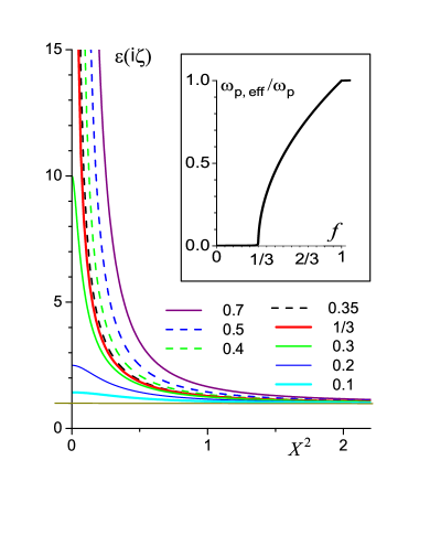
Figure 7: (Color online) The effective permittivity $\varepsilon_{\mathrm{eff}}(i\zeta)$ (in units of $\varepsilon_{\infty})$, for $d=3$ and different concentrations $f$ of the metal phase, as a function of the dimensionless variable $X^{2}=\zeta(\zeta+\gamma)/\omega_{p}^{2}$. Inset: effective plasma frequency $\omega_{p,\,\mathrm{eff}}$ (in units of $\omega_{p})$ versus $f$, in the coexistence region.

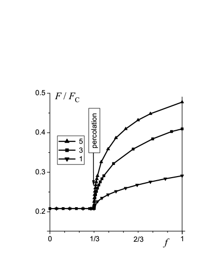
Figure 8: Casimir force for the interaction between two equivalent poor metals ($\nu=2)$ (with $\varepsilon_{\infty}=8$ and $\alpha=0.3$) versus the concentration $f$ of the metallic phase in the coexistence region. The force is normalized by values of the force $F_{\mathrm{C}}$ for ideal metals in the same geometry, and for different values of $l/\lambda_{p}$, where $\lambda_{p}$ is determined by the plasma frequency in the pure metallic phase.

To describe the Casimir force for such a nonuniform state, we have used the effective-medium approximation, EffMedia developed for composite metal-insulator media. This approximation has been used for explaining the optical properties of VO₂ near the metal-insulator transition.VO2 In this model, the effective value of $\varepsilon=\varepsilon_{\mathrm{eff}}(\zeta)$ is determined by the concentration $f$ ($0\leq f\leq 1$) of the metal phase following the equation,

$$f\cdot\frac{\varepsilon_{m}-\varepsilon_{\mathrm{eff}}}{\varepsilon_{m}+(d-1)\varepsilon_{\mathrm{eff}}}+(1-f)\cdot\frac{\varepsilon_{i}-\varepsilon_{\mathrm{eff}}}{\varepsilon_{i}+(d-1)\varepsilon_{\mathrm{eff}}}=0\;,$$ (21)

where $\varepsilon_{m}$ and $\varepsilon_{i}$ are the frequency-dependent permittivities for the metallic and insulating phases, respectively. Also, $d=2$ and $d=3$ for the thin film (thickness smaller then the grain size) and bulk sample, respectively. In the intermediate region, the effective permittivity $\varepsilon_{\mathrm{eff}}(i\zeta)$ as a function of the phase concentration $f$ can be written as follows:

$$2\frac{\varepsilon_{\mathrm{eff}}(i\zeta)}{\varepsilon_{\infty}}=(2f-1)\frac{\omega_{p}^{2}}{\zeta(\zeta+\gamma)}$$ (22)

$$+\sqrt{4+\frac{4\omega_{p}^{2}}{\zeta(\zeta+\gamma)}+\left[{\frac{(2f-1)\omega_{p}^{2}}{\zeta(\zeta+\gamma)}}\right]^{2}}\,\,{\rm for}\,\,d=2\,,$$

and

$$4\frac{\varepsilon_{\mathrm{eff}}(i\zeta)}{\varepsilon_{\infty}}=1+(3f-1)\frac{\omega_{p}^{2}}{\zeta(\zeta+\gamma)}+$$ (23)

$$+\sqrt{9+\frac{6(1+f)\omega_{p}^{2}}{\zeta(\zeta+\gamma)}+\left[{\frac{(3f-1)\omega_{p}^{2}}{\zeta(\zeta+\gamma)}}\right]^{2}}\,\,{\rm for}\,\,d=3\,.$$

These equations predict an infinite value of $\varepsilon_{\mathrm{eff}}(i\zeta)$ when $\zeta\to 0$ (that corresponds to a metallic conductivity) when $f_{c}\leq f\leq 1$ only, where $f_{c}=1/d$ is a percolation threshold, see Fig. 7. Otherwise, a dielectric behavior is present, with a finite value of $\varepsilon_{\mathrm{eff}}(i\zeta)$ when $\zeta\to 0,$

$$\varepsilon_{\mathrm{eff}}(\zeta=0)=\frac{\varepsilon_{\infty}}{1-fd}>\varepsilon_{\infty},\quad{\rm for}\quad f<\frac{1}{d}\,,$$

as shown in Fig. 7. In the metallic region (above the percolation threshold, for $f>f_{c})$, the behavior of $\varepsilon_{\mathrm{eff}}(i\zeta)$ at small $\zeta$ is determined by the effective plasma frequency $\omega_{p,\,\mathrm{eff}}$,

$$\varepsilon_{\mathrm{eff}}\to\varepsilon_{\infty}\frac{\omega_{p,\,\mathrm{eff}}^{2}}{\zeta(\zeta+\gamma)}\quad\mathrm{when}\ \zeta\to 0.$$

The value of $\omega_{p,\,\mathrm{eff}}^{2}$ increases linearly with $f$ from zero, at $f=f_{c}$, until $\omega_{p}^{2}$, at $f=1$. Thus, a square root behavior of the effective plasma frequency $\omega_{p,\,\mathrm{eff}}$ over $(f-f_{c})$ is present in the metallic region, see inset in Fig. 7.

It is useful to note here that a linear temperature dependence of $\omega_{p}^{2}$ was observed PhaseSep in La_0.7Sr_0.3MnO₃ for $T<T_{c}$. Thus, we can describe the Casimir force in the intermediate region as a series of curves, with their shape only depending on $l/\lambda_{p}$, as shown in Fig. 8.

IV Predictions for specific materials

Using the results obtained in the previous sections, here we estimate numbers for different materials showing the metal-insulator transition. To study the Casimir force in the vicinity of the metal-insulator transition, we choose two typical compounds: vanadium dioxide VO₂ and the manganites exhibiting colossal magnetoresistance. For these two materials, the general Drude behavior of permittivity, with typical values of $\lambda_{p}$ of the order of 1 $\mu$m and with relatively large values of $\varepsilon$, $\varepsilon_{\infty}\sim$ 5–10, is observed in the infrared region of interest.

IV.1 Vanadium dioxide VO₂

Vanadium dioxide, VO₂, shows a jump in the static conductivity (a metal-insulator transition) a little bit above room temperature, at $T=T_{c}\approx 68\ ^{\circ}$C. The pure metallic phase of VO₂ is realized at $T>88\ ^{\circ}$C, and pure insulator phase MIT (more exactly, semiconducting phase with a gap of the order of 1 eV) at $T<60\ ^{\circ}$C. For vanadium dioxide, the phase separated state has been observed VO2 within a finite temperature range, between 60 ^∘C and 88 ^∘C, by measuring the optical properties of VO₂. Recently, such state was directly observedDirCoexist via scanning tunneling spectroscopy. For all temperatures where the metallic conductivity is present, the generalized Drude behavior is observed up to the infrared frequency, with a relatively large value of $\varepsilon_{\infty}\cong 9$ and $\lambda_{p}=c/\omega_{p}\cong 1\ \mu$m. The phonon contribution to the value of $\varepsilon$, typical for the infrared region, is screened by free carriers, and the value of $\varepsilon_{\infty}\cong 9$ is kept until the high-frequency region, with $\lambda>\lambda_{0}\sim 0.1\ \mu$m, where the value of $(\varepsilon-1)$ vanishes. The value of the dissipation rate $\gamma$ for this compound is large enough, $\gamma/\omega_{p}\sim 0.3$ for VO₂, and the data for large $\alpha$ should be considered.

For VO₂, the Casimir force increases when increasing the temperature through the transition region, from 60 ^∘C until 88 ^∘C, see Fig. 9(a). The value of $\alpha$ is quite high, and the calculated change of the Casimir force is essentially smaller than for the naive estimate as the difference between the values $F_{\mathrm{C}}$ for an ideal metal and $F_{\mathrm{L}}$ for a dielectric, see Eqs. (1) and (2). The relative change of the Casimir force is maximal for large enough distances, e.g., $l\simeq 4\lambda_{p}\simeq$ $\mu$m.

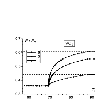
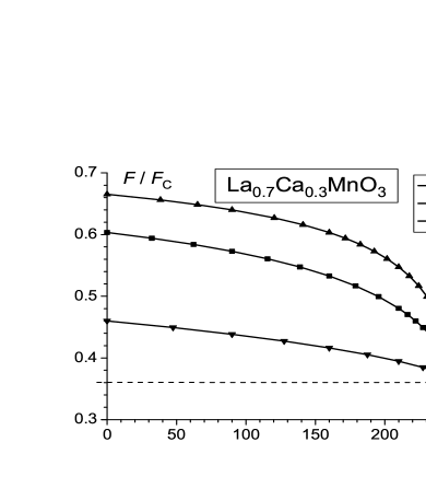
Figure 9: Predicted temperature dependence of the Casimir force for the interaction between a poor metal and an ideal metal, calculated for VO₂ (a) and for La_0.7Ca_0.3MnO₃ (b). The force is normalized by its value $F_{\mathrm{C}}$ for an ideal metal, for different values of $l/\lambda_{p}$=1, 3, 5, where $\lambda_{p}$ is determined by the plasma frequency in the pure metallic phase. The horizontal dashed lines indicate the limit values of the force for the pure insulating phase and (for VO₂ only) its metallic phase. The corresponding values of $F_{\mathrm{C}}$ are described by Eq. (1); for $\lambda_{p}\simeq 1.2\ \mu$m these are $F_{\mathrm{C}}=0.6\cdot 10^{-3}$, $0.74\cdot 10^{-5}$, and $0.965\cdot 10^{-6}$ Dyn/cm² for $l/\lambda_{p}$=1, 3, 5, respectively.

IV.2 Manganites.

Manganites (with antiferromagnetic insulators LaMnO₃ or NdMnO₃ as parent compounds, after substitution of La by divalent ion) show a metal-insulator transition at the dopant concentration $x\sim 0.3$, with a ferromagnetic metallic phase in the low temperature range. CMR These systems are very popular now in the context of colossal magnetoresistance, based on the possibility of the metal-insulator transition induced by an external magnetic field, that is caused by the ferromagnetic ordering of the metallic phase. On the other hand, the standard temperature-induced metal-insulator transition is possible for such materials as well. For example, the typical compound La_0.7Ca_0.3MnO₃ demonstrates a metal-insulator transition at $T=T_{c}$ = 250 K. The phase separation state is present for all temperatures below the transition point, and the typical linear dependence of $\omega_{p,\,\mathrm{eff}}^{2}$ has been observed EffMedia in this region. Note that this metal-insulator transition is accompanied by ferromagnetic ordering. In principle, it could produce an extra-force of magnetic origin near the transition (antiferromagnetic ordering, present for some metal-insulator transition, does not produce any source of long-ranged interactions). However, for large enough plane-parallel samples, the magnetic flux lines are closed inside the magnetic sample, and should not produce any serious parasitic effects. For these compounds, $\omega_{p}$ is small and the corresponding $\lambda_{p}\sim 1\ \mu$m. The main specific feature important for us here is the low value of the dissipation rate: typical values of $\gamma/\omega_{p}$ are $\sim$ 0.02–0.05, and the low-$\gamma$ behavior of the curves shown in Figs. 2, 3 are adequate.

For La_0.7Ca_0.3MnO₃, the metallic phase corresponds to the low-temperature range, and the value of the force increases when decreasing the temperature, which leads to an opposite temperature behavior of the Casimir force, compared to VO₂. The value of $\alpha$ for this compound is relatively low, and the temperature dependence of the Casimir force is sharper than for the previous example. One more specific feature is the presence of phase separation in the whole region of the metallic phase existence. Thus, one can expect an essential dependence of the Casimir force for all temperatures below the transition temperature, see Fig. 9(b).

V Conclusions

The Casimir force depends on the materials used, and we have studied some of these material-dependent aspects. The Casimir force $F_{\mathrm{C}}$ for a mechanical system containing compounds with a metal-insulator transition shows an abrupt temperature dependence in the transition region. The relative change of the force $\Delta F_{\mathrm{C}}$ when crossing the transition region can be quite large, of the order of the force itself for a distance $\sim$ 5–6 microns. The relative change $\Delta F_{\mathrm{C}}$ of the Casimir force is larger for large distances, where the absolute value of the force is small, but even for a distance $l=\lambda_{p}=1.2\ \mu$m it reaches 30%. The dependence of the force on temperature is sharp near the percolation threshold, where the static metallic conductivity appears.

When measuring such tiny forces, the exclusion of any parasitic effects, like electrostatic forces, is essential. To avoid electrostatic forces, the usual highly-conducting samples are short-circuited. 11 This method might appear to be ineffective for the metal-insulator transition compounds near the insulating region. However, such compounds are more semiconducting than insulating in this region and the conductivity is non-zero at room temperatures. Thus, we believe that the same technique could be used. To increase the conductivity in the semiconducting region, the usual doping by donor or acceptor impurities could be used. Finally, we note that the metal-insulator transition is sometimes accompanied by structural phase transitions, which could lead to some lattice distortions. Thus, care should be taken to choose materials and operating conditions that avoid these additional difficulties.

For measurement of the Casimir force for samples made with usual metals, small separations are preferable. The creation of experimental set-ups with very small (sub-micrometer) distances between samples is a serious challenge for experimentalists. As follows from our analysis, distances $l$ larger than the plasma wavelength $\lambda_{p}$ are preferable for the experimental observation of the effects, we predict around the region of the metal-insulator transition. For the compounds discussed above, this means distances of the order of (2–4) $\mu$m. In the planned experiments Exper07 for measuring the Casimir force using Vanadium oxide samples, the separations are (0.2–0.4) $\mu$m, which equals (0.1–0.3) $\lambda_{p}$. These values are much smaller than the optimal values noted above. For separations $l$ of the order of (0.1–0.3) $\lambda_{p}$, the Casimir force should follow low-$l$ asymptotics for any temperature (in both the metallic and the insulating phases). The temperature dependence of the Casimir force should be weak and the manifestation of the metal-insulator transition should be minor for such an experimental set-up.

- (1) H. B. G. Casimir, Proc. Kon. Nederl. Akad. Wet. 51, 793 (1948).
- (2) P. W. Milonni, The Quantum Vacuum (Academic press, San Diego, 1994).
- (3) K. A. Milton, The Casimir Effect: Physical Manifestations of Zero-point Energy (World Scientific, Singapure, 2001).
- (4) M. Kardar and R. Golestanian, Rev. Mod. Phys. 71, 1233 (1999).
- (5) M. Bordag, U. Mohideen, and V. M. Mostepanenko, Phys. Reports 353, 1 (2001).
- (6) F. Capasso, J. N. Munday, D. Iannuzi, and H. B. Chan, IEEE J. Sel. Top. Quant. El. 13, 400 (2007).
- (7) S. K. Lamoreaux, Rep. Progr. Phys. 68, 201 (2005); S. K. Lamoreaux, Phys. Today 60, No. 2, 40 (2007).
- (8) C. Cattuto, R. Brito, U. Marini Bettolo Marconi, F. Nori, and R. Soto, Phys. Rev. Lett. 96, 178001 (2006).
- (9) J. M. Obrecht, R. J. Wild, M. Antezza, L. P. Pitaevskii, S. Stringari, and E. A. Cornell, Phys. Rev. Lett. 98, 063201 (2007).
- (10) S. K. Lamoreaux, Phys. Rev. Lett. 78 5 (1997).
- (11) U. Mohideen and A. Roy, Phys. Rev. Lett. 81, 4549 (1998); A. Roy and U. Mohideen, Phys. Rev. Lett. 82, 4380 (1999); F. Chen and U. Mohideen, Phys. Rev. Lett. 88, 101801 (2002); F. Chen, G. L. Klimchitskaya, U. Mohideen, and V. M. Mostepanenko, Phys. Rev. A69, 022117 (2004).
- (12) D. Iannuzzi, M. Lisanti, J. N. Munday, and F. Capasso, Solid State Commun. 135, 618 (2005); J. N. Munday, D. Iannuzzi, Yu. Barash, and F. Capasso, Phys. Rev. A71, 042102 (2005); J. N. Munday, D. Iannuzzi, and F. Capasso, New J. Phys. 8, 244 (2006); D. Iannuzzi, M. Lisanti, J. N. Munday, and F. Capasso, J. Phys. A: Math. Gen. 39, 6445 (2006); J. N. Munday and F. Capasso, Phys. Rev. A75, 060102(R) (2007).
- (13) C. Genet, A. Lambrecht and S. Reynaud, Phys. Rev. A 62, 012110 (2000).
- (14) G. Bressi, G. Carugno, R. Onofrio, and G. Ruoso, Phys. Rev. Lett. 88, 041804 (2002).
- (15) V. Petrov, M. Petrov and V. Bryksin, J. Petter and T. Tschudi, Opt. Lett. 31, 3167 (2006).
- (16) H. B. Chan, V. A. Aksyuk, R. N. Kleiman, D. J. Bishop, and F. Capasso, Science 291, 1941 (2001); H. B. Chan, V. A. Aksyuk, R. N. Kleiman, D. J. Bishop, and F. Capasso, Phys. Rev. Lett. 87, 211801 (2001).
- (17) E. M. Lifshitz, Sov.Phys. - JETP 2, 73 (1956).
- (18) E. M. Lifshitz, L. P. Pitaevskii, Statistical Physics, Part 2 (Pergamon Press, Oxford, 1980).
- (19) I. E. Dzyaloshinskii, E. M. Lifshitz, L. P. Pitaevskii, Sov. Phys. Usp. 4, 153 (1961).
- (20) F. Chen, U. Mohideen, G. L. Klimchitskaya, and V. M. Mostepanenko, Phys. Rev. A 72, 020101(R) (2005); Phys. Rev. A 74, 022103 (2006); F. Chen, G. L. Klimchitskaya, V. M. Mostepanenko, and U. Mohideen, Phys. Rev. Lett. 97, 170402 (2006); Phys. Rev. B 76, 035338 (2007).
- (21) R. Castillo-Garza, C.-C. Chang, D. Jimenez, G. L. Klimchitskaya, V. M. Mostepanenko, and U. Mohideen, Phys. Rev. A 75, 062114 (2007).
- (22) J. Blocki, J. Randrup, W. J. Swiatecki, and C. F. Tsang, Ann. Phys. (N.Y.) 105, 427 (1977).
- (23) D. E. Krause, R. S. Decca, D. López, and E. Fischbach, Phys. Rev. Lett. 98, 050403 (2007).
- (24) V. A. Yampol’skii, S. Savel’ev, Z. A. Mayselis, S. S. Apostolov, and F. Nori, arXiv: cond-mat.mes-hall/0712.1395v1.
- (25) F. S. S. Rosa, D. A. R. Dalvit, and P. W. Milonni, Phys. Rev. Lett. 100, 183602 (2008).
- (26) N. F. Mott, Metal-Insulator Transitions, 2 ed. (Taylor&Francis, London, 1990); M. Imada, A. Fujimori, Y Tokura, Rev. Mod. Phys., 70, 4 (1998).
- (27) High Temperature Superconductivity, edited by K. S. Bedell, D. Coffey, D. E. Meltzer, D. Pines, and J. R. Schrieffer (Addison-Wesley, Reading, MA, 1990).
- (28) Physics of Manganites, edited by T. A. Kaplan and S. D. Mahanti (Kluwer Academic/Plenum publishers, New York, 1999).
- (29) T. W. Noh, P. H. Song, and A. J. Sievers, Phys. Rev. B 44, 5459 (1991).
- (30) H. S. Choi, J. S. Ahn, J. H. Jung, and T. W. Noh, and D. H. Kim, Phys. Rev. B 54, 4621 (1996).
- (31) Y. J. Chang, C. H. Koo, J. S. Yang, Y. S. Kim, D. H. Kim, J. S. Lee, T. W. Noh , H. T. Kim, and B. G. Chae, Thin Solid Films, 486 46 (2005).
- (32) K. H. Kim, J. H. Jung, and T. W. Noh, Phys. Rev. Lett. 81, 1517 (1998).