Kinetics of water flow through polymer gel

Abstract

The water flow through the poly(acrylamide) gel under a constant water pressure is measured by newly designed apparatus. The time evolution of the water flow in the gel, is calculated based on the collective diffusion model of the polymer network coupled with the friction between the polymer network and the water. The friction coefficient are determined from the equilibrium velocity of water flow. The Young modulus and the Poisson’s ratio of the rod shape gels are measured by the uni-axial elongation experiments, which determine the longitudinal modulus independently from the water flow experiments. With the values of the longitudinal modulus and of the friction determined by the experiments, the calculated results are compared with the time evolution of the flow experiments. We find that the time evolution of the water flow is well described by a single characteristic relaxation time predicted by the collective diffusion model coupled with the water friction.

1 Introduction

The gel is an important state of matter that is found in a wide variety of biological, chemical, and food systems TanakaSci . The polymer gel consists of a cross-linked polymer network and a large amount of solvent (typically water). Since the average mesh size (the distance between neighboring crosslinks) of the polymer network is in general large compared to small molecules, they can pass through the gel easily. Two different transport processes are important in the gel.

The first one is the diffusive flow of molecules Muhr . The transport of molecules by the diffusion in the polymer network is modeled as the diffusion of the probe objects in the fixed mesh of obstacles. The ratio between the probe size and the mesh size plays essential role to determine the diffusion coefficient of the molecules in the gels. The diffusion of the probe molecules in the gel has been measured by the pulsed field gradient nuclear magnetic resonance. The results indicate that the diffusion coefficient of the probe molecules of various sizes in the gel is well described by a simple scaling relationship TokitaPRE .

The second process is the convective flow of the water through the polymer network TokitaJCP95 ; TokitaSci ; TokitaAPS . When the water flows in the gel, it experiences the hydrodynamic friction from the polymer network, at the same time, the polymer network of gel is deformed from the initial configuration by the drag force of the water. The entire flowing process of the water is determined by the balance between the viscoelastic response of the water flow and that of the polymer network. The collective diffusion of the polymer network coupled with water friction, therefore, plays essential roles in the convective flow process in the gel.

As well as the transport phenomena in the gel, the water flow is also important in the kinetics of the volume phase transition of the gel including the pattern formations in shrinking gelsTanakaPRL ; TanakaJCP70 ; Matsuo ; TokitaJPSJ ; MaskawaJCP ; TakigawaJCP111 ; TokitaJCP113 ; TakigawaJCP117 ; BoudaoudPRE ; UrayamaJCP ; NosakaPoly . Kinetics of solvent flow in the gel is the main subject of the application of the gel to control the solvent flow YoshikawaJJAP ; SuzukiJCP . Although the significance, the solvent flow process in the polymer gel has yet to be studied in detail.

It is the purpose of this paper to describe the kinetics of the water flow through the polymer gel, based on the collective diffusion model coupled with water friction. The characteristic relaxation time of the water flow process in the gel is expressed as $\tau=L^{2}/\pi^{2}D_{c}$ with the parameters: the typical size of the gel, $L$, and the collective diffusion coefficient of the polymer network, $D_{c}$. The collective diffusion coefficient is expressed by using the longitudinal modulus of the gel, $\kappa$, and the friction coefficient between the polymer network and the water, $f$, as TanakaJCP70 ; TanakaJCP59

$$D_{c}=\frac{\kappa}{f}.$$ (1)

The water flow in the polymer network is, thus, directly governed by the viscoelastic property of the gel. The collective diffusion coefficient of polymer gels has been extensively measured by quasi-elastic light scattering Munch1 ; Munch2 . The friction coefficient between the polymer network of gel and the water has been measured by flowing the water through the gel TokitaJCP95 ; TokitaSci ; TokitaAPS .

In this paper, we present experimental results on the water flow through the gel, and show that the time evolution of the water flow through the gel is described satisfactorily by the collective diffusion model of polymer network with water friction. The information on the kinetics of water flow in the gel will help the better use of them in the applications.

2 Experiment

2.1 Water flow measurements

The experimental setting of the water flow measurements is illustrated schematically in Figure 1.

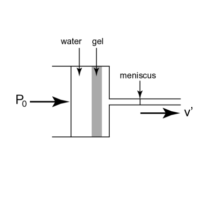
Figure 1: Experimental setting of water flow measurements

A thin circular slab gel of thickness, $L$, is set in a tube and the rim of the gel is glued to the tube. The surface of the gel at the lower reaches side is mechanically fixed to the end plate through an O-ring. When the small pressure, $P_{0}$, is applied to the water from the upper stream side of the gel, the water flows through the gel deforming the polymer network of gel by the drag force. The macroscopic value of the friction coefficient of the gel, $f$, is determined from the velocity of the water flows out of the gel in the equilibrium state, $v_{\infty}$, as

$$f=\frac{P_{0}}{v_{\infty}L}.$$ (2)

Even though the concept is simple, the mechanical measurement of the friction coefficient between the polymer network of gel and the water is not easy because the friction of the gel is huge. The difficulty of evaluating the friction coefficient measured from the water flow through the gel is described in the reference TokitaJCP95 . In our experiments, the difficulty is overcome by using a well calibrated homogeneous glass capillary to amplify the velocity of water as shown in Figure 1. The position of the meniscus of water in the capillary is measured as a function of time after the pressure is applied to the water.

The photographs of the apparatus used in this study are given in Figure 2.

Figure 2: Apparatus for water flow measurements: (a) the upper photograph shows the external appearance, (b) the lower photographs shows the inside of the end plates.

The essential structure of the apparatus is the same with the previous one but some points are improved for the precise measurements of the friction of the gel TokitaJCP95 . The right hand side of Figure 2 (a) is the upper stream side and is connected to a water column to apply the hydrostatic pressure. The glass capillary is set at the top of stainless steel pipe which can be seen at the left hand side of Figure 2 (a). Leak of water around the gel is prevented by setting O-rings inside the cell as shown in Figure 2 (b). All parts of the cell is made of stainless steel to avoid the mechanical deformation due to the applied pressure. The mechanical deformation of the apparatus is considerably reduced compared to the previous one.

2.2 Mechanical response measurements

The mechanical response of the polymer gel relates the friction coefficient to the collective diffusion coefficient of the polymer network as $D_{c}=\kappa/f$ where $\kappa=K+\frac{4\mu}{3}$ TanakaJCP59 . Here, $\kappa$ is the longitudinal modulus of the gel and $K$ and $\mu$ are the bulk modulus and the shear modulus of the gel, respectively. We measure two elastic moduli of the gel simultaneously, and the longitudinal modulus of the gel is determined from them.

The rod shape gel is elongated in water at a strain of about 10 $\%$ and the stress is measured. The size of the gel is observed by using a microscope during the elasticity measurements to obtain the Young’s modulus of the gel, $E$, and the Poisson’s ratio, $\sigma$. The longitudinal modulus of the gel, $\kappa$, is determined from the Young’s modulus and the Poisson’s ratio by $\kappa=K+\frac{4\mu}{3}$, $K=E/3(1-2\sigma)$ and $\mu=E/2(1+\sigma)$.

In this short time experiments, the water solvent neither goes out nor comes into the gels. Thus we determine the mechanical response of the gel independently from the friction experiments by the water flow. We use the results to analyze the kinetics of water flow through the polymer network.

2.3 Sample

The samples used in this paper are poly(acrylamide) gel that is obtained by the radical co-polymerization of the main-chain component, acrylamide, and the cross-linker, N,N’-methylene-bis-acrylamide. The concentration of the gel used in this measurement is 1 M. Ammoniumpersulfate and N,N,N’,N’-tetramethyl-ethylenediamine are used as the initiator and the accelerator. All chemicals used here are of electrophoresis grade, purchased from BioRad and used without further purification. The gel for the friction measurements is prepared in the circular gel mold, where the gel-bond films (FMC) with circular opening are glued on the both sides. For the friction coefficient measurements, the gel is prepared in the measurement cell and kept under water at a constant room temperature for overnight to reach the equilibrium state.

For the elastic modulus measurements, the rod shaped gels are prepared in the capillary. The desired amounts of the main-chain component, the cross-linker, and the accelerator are dissolved into the distilled and de-ionised water, which is prepared by a Mili-Q system. The pre-gel solution is de-gassed for 20 min, and then the desired amount of the initiator is added to the solution to initiate the reaction. The sample gels are taken out of the reaction bath and then washed by distilled and de-ionized water extensively and used in each measurement.

3 Experimental results

3.1 Friction coefficient of gel

The experimental results of the measurement of water flow through the gel are shown in Figure 3.

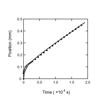
Figure 3: Position of meniscus in capillary fit by equation (19) with $a$ and $b$ as adjusted parameters.

The position of the meniscus in the capillary of $10\mu l$ glass micro-pipette is plotted as a function of the time elapsed after the application of the pressure to the water. The slope of the flow curve, thus obtained, represents the water velocity in the capillary, $v^{\prime}$. The velocity of the flow is high at first. Then it eventually decreases with time and approaches to an equilibrium value. The equilibrium state is attained about 5 to 7 $\times$ 10³ s after the pressure is applied to the water. The velocity of the meniscus in the equilibrium state is determined by the least-squares analysis of the linear portion of the flow curve in Figure 3, typically in the time region more than 1 $\times$ 10⁴ s, that yields to $v^{\prime}_{\infty}=1.9\times 10^{-7}$ m/s. The velocity of water flow in the gel, $v$, is then calculated from the velocity of the meniscus, $v^{\prime}$, with the ratio of the radius of the circular opening of the gel mold, $R$, and that of the capillary, $r$, as $v=v^{\prime}(r/R)^{2}$. The values of $R$ and $r$ are measured as 1.745 mm and 0.268 mm, respectively. The equilibirium velocity of water flow in the gel is, thus, calculated as $v_{\infty}=4.4\times 10^{-9}$ m/s. The pressure applied to the water is $P_{0}=2.9\times 10^{3}$ N/m², which corresponds to the height of water column of 30 cm, and the thickness of the gel is $L=1.0\times 10^{-3}$ m. From these values, the friction coefficient of the gel is calculated by equation (2) that yields to $f=6.6\times 10^{14}$ N s/m⁴. This agrees with a typical value of the friction coefficient of the transparent poly(acrylamide) gel evaluated by other experiments TokitaJCP95 .

3.2 Elastic modulus of gel

In Figure 4, we show the concentration dependence of the Young’s modulus and the Poisson’s ratio of the gels used in our experiment.

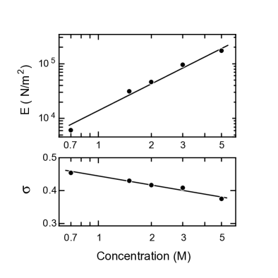
Figure 4: Concentration dependence of elastic moduli: (a) the upper graph shows Young’s modulus, $E$, (b) the lower graph shows Poisson’s ratio, $\sigma$.

The least-squares analysis of the results yields that the concentration dependence of the Young’s modulus of the gel is well described by a power law relationship with a scaling exponent of 1.7, which is slightly smaller than the value expected from the scaling argument deGennes . The Poisson’s ratio is about 0.45 in the dilute gels. It decreases with the concentration of the gel and reaches to about 0.35 at higher concentration region. The values of the Poisson’s ratio of the dilute gels are close to those of the incompressible materials. On the other hand, the values of the Poisson’s ratio of the dense gels are rather close to those of the metals and the glasses. The Young’s modulus and the Poisson’s ratio of the gel at a concentration of 1 M is observed as $E=1.3\times 10^{4}$ N/m² and $\sigma=0.44$, respectively. The longitudinal modulus is then calculated as $\kappa=4.1\times 10^{4}$ N/m² for the gel at a concentration of 1 M. Our results are consistent with previously published Poisson’s ratio of poly(acrylamide) gels and a theory TakigawaPJ1 ; TakigawaPJ2 .

The diffusion coefficient of the polymer network is deduced from equation (1) as $D_{c}=6.2\times 10^{-11}$ m²/s, which agrees with a typical value of the diffusion coefficient of the transparent poly(acrylamide) gel evaluated by other experiments TanakaJCP70 ; TanakaJCP59 ; Munch1 ; Munch2 .

4 Kinetics of water flow through gel

When the water flows in the gel (polymer network) by the application of the mechanical pressure, the polymer network of gel deforms from the initial position by the drag force of the water flow. We introduce a function, $u(x,t)$, that represents the displacement of a point in the polymer network from its initial position at $x$. We assume $u$ is always small compared to the characteristic size of the gel, $L$. Under the present definition, $u(x,t)=0$ at $t=0$. We also assume that the macroscopic velocity of the water in the polymer network, $v(t)$, and microscopic friction coefficient, $f$, are uniform in space.

$$\frac{\partial v}{\partial x}=0.$$ (3)

Then, we write down the equation of motion of the polymer network and that of the water in the gel as

$$\rho_{g}\ddot{u} = -f(\dot{u}-v)+\kappa\frac{\partial^{2}u}{\partial x^{2}},$$ (4)

$$\rho_{w}\dot{v} = f(\dot{u}-v)-\frac{\partial P}{\partial x},$$ (5)

where $\rho_{g}$ and $\rho_{w}$ are the density of the polymer network and that of the water, respectively; A dot over the variable denotes the time derivative; $P(x,t)$ represents the pressure inside the region that the gel occupied.

By neglecting the inertia terms in equations (4) and (5), we obtain

$$\kappa\frac{\partial^{2}u}{\partial x^{2}}-\frac{\partial P}{\partial x}=0,$$ (6)

and

$$f(v-\dot{u})=-\frac{\partial P}{\partial x}.$$ (7)

A set of equations (3), (6), (7) corresponds to one dimensional case under a limit of small polymer volume fraction $\phi\rightarrow 0$ of a general description for 3 dimensional deformation of gelsYamaue ; Doi .

In our experimental setup of water flow measurement in Fig.1, we see $P(x=0,t)=P_{0}$ and $P(x=L,t)=0$. Taking a spacial average of equation (7) over the space the gel occupied, we obtain

$$v-\frac{1}{L}\int_{0}^{L}\dot{u}dx=\frac{P_{0}}{Lf}.$$ (8)

The time evolution of water flow in the gel $v(t)$ is determined locally from $u(x,t)$ by

$$v=\dot{u}-D_{c}\frac{\partial^{2}u}{\partial x^{2}}.$$ (9)

Here, we use the collective diffusion coefficient of the gel, $D_{c}$, defined in equation (1). The displacement of polymer network $u(x,t)$ is, hence, determined by solving the equation:

$$\dot{u}-\frac{1}{L}\int_{0}^{L}\dot{u}dx=D_{c}\frac{\partial^{2}u}{\partial x^{2}}+\frac{P_{0}}{Lf}.$$ (10)

In the equilibrium state, $\dot{u}(x,t)\rightarrow 0$ as $t\rightarrow\infty$. The restoring force due to the deformation of the polymer network is in balance with constant gradient of the pressure. In the equilibrium state, therefore, equations (3), (6), (7), (8) give

$$\frac{\partial^{2}u(x,t=\infty)}{\partial x^{2}}=-\frac{P_{0}}{D_{c}Lf}.$$ (11)

The displacement, $u(x,t)$, satisfies the following boundary conditions:

$$u(L,t) = 0,$$ (12)

$$\frac{\partial u(0,\infty)}{\partial x} = 0.$$ (13)

Integration of equation (11) with respect to $x$ with the boundary conditons yields

$$u(x,\infty)=\frac{P_{0}}{2D_{c}Lf}(L^{2}-x^{2}).$$ (14)

Solving equation (10) under the above boundary conditions, we obtain the displacement, $u(x,t)$, as (See Appendix)

$$u(x,t)=\sum_{n}\frac{2v_{\infty}\tau}{n^{2}}\left[(-1)^{n}\left(\cos{\frac{n\pi}{L}x}-1\right)\right]\exp{\left(-\frac{n^{2}}{\tau}t\right)},$$ (15)

where

$$\tau = \frac{L^{2}f}{\pi^{2}\kappa},$$ (16)

$$v_{\infty} = \frac{P_{0}}{Lf}.$$ (17)

The velocity of the water flow, $v(t)$, is derived from equation (7) as

$$v=v_{\infty}\left[1+2\sum_{n=1}^{\infty}\exp\left(-\frac{n^{2}}{\tau}t\right)\right]=v_{\infty}\theta_{3}(0,e^{t/\tau}),$$ (18)

where $\theta_{3}(u,q)$ is the elliptic theta function. The position of meniscus is expressed as

$$a\left[t-2\sum_{n=1}^{\infty}\frac{\tau}{n^{2}}\exp\left(-\frac{n^{2}}{\tau}t\right)\right]+b,$$ (19)

where $b$ is the initial position, and

$$a=\left(\frac{R}{r}\right)^{2}v_{\infty}.$$ (20)

5 Discussion

Now we compare the experimental results with the theoretical predictions by equations (18) and (19). The values obtained by the experimental measurements are, $L=1.0\times 10^{-3}$ m, $\kappa=4.1\times 10^{4}$ N/m², and $f=6.6\times 10^{14}$ Ns/m⁴, respectively.

By applying these values into equation (16), we obtain the characteristic relaxation time $\tau=1.6\times 10^{3}$ s. The equilibrium velocity of water flow in the gel observed by the experiments is, as is already given in the section 3, $v_{\infty}=4.4\times 10^{-9}$ m/s. From equation (14) the deformation of gel is estimated as 3.5$\%$ which is consistent with our assumption of small $u$.

The time evolution of the water flow is then calculated by equation (18) with above experimental values. The results are given in Figure 5.

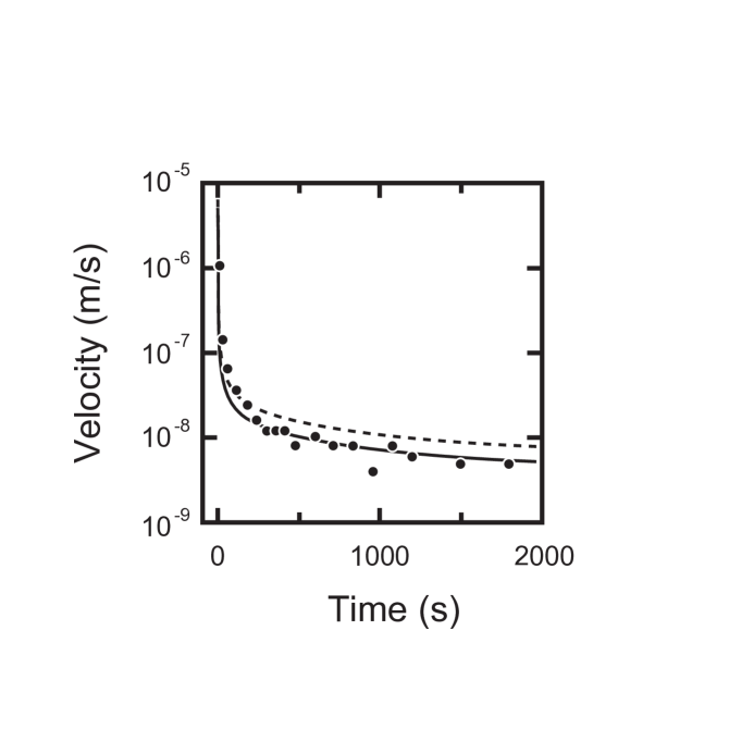
Figure 5: Water flow velocity in gel: (a) the solid line corresponds to the theoretical curve fitting all the data, (b) the dotted line corresponds to the theoretical curve expected from the short time data ($<$200s).

The normalized velocity of the water flow in the gel is also calculated from the slope of the flow curve in Figure 3 and shown in Figure 5. We find that the time evolution of the velocity of water flow in the gel is well explained by the equation (18) with a single characteristic relaxation time $\tau$.

However, there is a slight discrepancy in the time evolution curve of the velocity at a short time range ($<$200s) between the theory and the experimental results as one can see in figure 3 and 5. The absolute value of the equilibrium velocity determined from the short time data ($<$200s) of the friction experiment is smaller than that determined by including the long time data. Figure 5 shows that the deference between those two values is roughly 20 $\%$.

It would be worth noting that the theory predicts that the water flow creates a uni-axial deformation of polymer network, i.e., the one dimensional concentration gradient in the gel, proportional to

$$\left(1+\frac{\partial u(x,\infty)}{\partial x}\right)^{-1}\approx 1+\frac{P_{0}x}{D_{c}Lf}.$$ (21)

The compression of gel is the cause of the initial rapid water flow. It is reported that the friction of the homegeneous gel depends on the polymer volume fraction, $\phi$, as $f\propto\phi^{1.5}$ TokitaJCP95 ; deGennes . The friction, therefore, is expected to increase according to the compression of the gel by the water flow. The increment of the friction may explain the difference between the short time data and long time data. The difference between the estimated equilibrium water velocities corresponds to 14 $\%$ homogeneous compression of the sample slab gel, which is larger than the deformation which the present theory estimates. Unfortunately, we cannot measure the deformation of the gel under the water flow with the current experimental setup.

6 Conclusion

The kinetics of the water solvent flow through the polymer network of gel is measured experimentally and described by a simple phenomenological theory. The experiment shows that the equilibrium state is reached after long time and that the friction of the gel shows a large value. The time evolution of the velocity of the water flow in the gel is calculated on the basis of the collective diffusion model of the polymer network coupled with the water friction, assuming both the water velocity and the friction coefficient between the polymer network and the water are uniform in the gel. The theory reproduces the time evolution of the water flow of the experiments for thin dilute gel fairly well with a single characteristic relaxation time. We are able to deduce the collective diffusion coefficient from the water flow experiment on gels.

However there is a difference between experimental value of the equilibrium velocity and the value expected from the theoretical calculation by using parameters obtained from the short time flow measurements and the mechanical measurements. It suggests that the inhomogeneity of the friction and the concentration of the gel under the water flow might be important for the kinetics of the water flow. A better microscopic model is required for complete understanding of water flow through gel beyond the phenomenological understanding presented in this paper.

APPENDIX A: Solution of the equation of motion

We define a function $W(x,t)$ as a deviation from the equilibrium displacement:

$$u(x,t)-\int v(t)dt\equiv W(x,t)+u(x,\infty).$$ (22)

We obtain an equation for $W(x,t)$ from equation (10) as

$$\frac{\partial W}{\partial t}=D_{c}\frac{\partial^{2}W}{\partial x^{2}}.$$ (23)

By assuming $W(x,t)=X(x)T(t)$, the equation (23) becomes

$$\dot{T}(t) = -\lambda^{2}D_{c}T(t),$$ (24)

$$\frac{d^{2}X(x)}{dx^{2}} = -\lambda^{2}X(x),$$ (25)

where $\lambda$ is a constant. The general solution for $W(x,t)$ would be

$$W(x,t) = \sum_{n=1}^{\infty}\left[A_{n}\cos\lambda_{n}x+B_{n}\sin\lambda_{n}x\right]$$ (26)

$$\times\exp(-\lambda_{n}^{2}D_{c}t)+A_{0}x+B_{0}.$$

The boundary conditions for $W(x,t)$ are

$$\left.\frac{du}{dx}\right|_{x=0}=0 \longrightarrow \left.\frac{dW}{dx}\right|_{x=0}=0,$$ (27)

$$\left.\frac{du}{dt}\right|_{t=\infty}=0 \longrightarrow \left.\frac{dW}{dt}\right|_{t=\infty}=v(\infty),$$ (28)

$$u(L,t)=0 \longrightarrow W(L,t)=-\int vdt.$$ (29)

The boundary condition (27) yields

$$\left.\frac{dW}{dx}\right|_{x=0} = \sum_{n=1}^{\infty}[A_{n}(-\lambda_{n}\sin\lambda_{n}x)+B_{n}(\lambda_{n}\cos\lambda_{n}x)]$$

$$\left.\times\exp(-\lambda_{n}^{2}D_{c}t)\right|_{x=0}+B_{0}$$

$$= \left.\sum_{n=1}^{\infty}[A_{n}(-\lambda_{n}\times 0)+B_{n}(\lambda_{n}\times 1)]\exp(-\lambda_{n}^{2}D_{c}t)\right|_{x=0}$$

$$+B_{0}$$

$$= 0.$$

This indicates $B_{n}=0$.

The boundary condition (28) yields

$$\left.\frac{dW}{dx}\right|_{t=\infty} = \left.\sum_{n=1}^{\infty}[A_{n}\cos\lambda_{n}x](-\lambda_{n}^{2}D_{c})\exp(-\lambda_{n}^{2}D_{c}t)\right|_{t=\infty}+A_{0}$$

$$= v(\infty).$$

This indicates that the constant, $\lambda_{n}^{2}$, should be positive, $\lambda_{n}^{2}>0$ for $n\geq 1$ and $A_{0}=v(\infty)$. Finally, the boundary condition (29) yields

$$W(L,t) = \sum_{n=1}^{\infty}[A_{n}(\cos\lambda_{n}L+C_{nA})]\exp(-\lambda_{n}^{2}D_{c}t)+A_{0}L+B_{0}$$

$$= -\int vdt.$$

This indicates $C_{nA}=-\cos\lambda_{n}L$. The following relationships for $B_{n}$, $\lambda_{n}^{2}$, and $C_{nA}$ are obtained:

$$B_{n} = 0,$$ (30)

$$\lambda_{n}^{2} > 0,$$ (31)

$$C_{nA} = -\cos\lambda_{n}L.$$ (32)

And $W(x,t)$ becomes

$$W(x,t)=\sum_{n=1}^{\infty}[A_{n}(\cos\lambda_{n}x+C_{nA})]\exp(-\lambda_{n}^{2}D_{c}t).$$ (33)

Substitution of this solution (33) into equation (23) yields

$$\sum_{n=1}^{\infty}[A_{n}(\cos\lambda_{n}x+C_{nA})](-\lambda_{n}^{2}D_{c})\exp(-\lambda_{n}^{2}D_{c}t)$$

$$-\frac{1}{L}\int_{0}^{L}\sum_{n=1}^{\infty}[A_{n}(\cos\lambda_{n}x+C_{nA})]$$

$$\times(-\lambda_{n}^{2}D_{c})\exp(-\lambda_{n}^{2}D_{c}t)dx$$

$$=D_{c}\sum_{n=1}^{\infty}A_{n}\lambda_{n}^{2}(-\cos\lambda_{n}x)\exp(-\lambda_{n}^{2}D_{c}t).$$ (34)

The first term of the left handed member (LHM1) is written as follows:

$${\rm LHM1}= \sum_{n=1}^{\infty}(-\lambda_{n}^{2}D_{c})A_{n}(\cos\lambda_{n}x)\exp(-\lambda_{n}^{2}D_{c}t)$$

$$+ \sum_{n=1}^{\infty}(-\lambda_{n}^{2}D_{c})(A_{n}C_{nA})\exp(-\lambda_{n}^{2}D_{c}t).$$

The second term of the left handed member (LHM2) is expressed as follows:

$${\rm LHM2}= - \frac{1}{L}\int_{0}^{L}\sum_{n=1}^{\infty}(-\lambda_{n}^{2}D_{c})(A_{n}\cos\lambda_{n}x)$$

$$\times\exp(-\lambda_{n}^{2}D_{c}t)dx$$

$$- \frac{1}{L}\int_{0}^{L}\sum_{n=1}^{\infty}(-\lambda_{n}^{2}D_{c})(A_{n}C_{nA})\exp(-\lambda_{n}^{2}D_{c}t)dx.$$

The first term of LHM2 is expressed as

$$- \frac{1}{L}\int_{0}^{L}\sum_{n=1}^{\infty}(-\lambda_{n}^{2}D_{c})(A_{n}\cos\lambda_{n}x)\exp(-\lambda_{n}^{2}D_{c}t)dx$$

$$= - \left.\frac{1}{L}\sum_{n=1}^{\infty}(-\lambda_{n}^{2}D_{c})\frac{1}{\lambda_{n}}(A_{n}\sin\lambda_{n}x)\exp(-\lambda_{n}^{2}D_{c}t)\right|_{0}^{L}$$

$$= - \frac{1}{L}\sum_{n=1}^{\infty}(-\lambda_{n}^{2}D_{c})\frac{1}{\lambda_{n}}(A_{n}\sin\lambda_{n}L)\exp(-\lambda_{n}^{2}D_{c}t).$$

The second term of LHM2 becomes

$$- \frac{1}{L}\int_{0}^{L}\sum_{n=1}^{\infty}(-\lambda_{n}^{2}D_{c})(A_{n}C_{nA})\exp(-\lambda_{n}^{2}D_{c}t)dx$$

$$= - \sum_{n=1}^{\infty}(-\lambda_{n}^{2}D_{c})(A_{n}C_{nA})\exp(-\lambda_{n}^{2}D_{c}t).$$

Hence, the equation (34) is reduced to

$$-\frac{1}{L}\sum_{n=1}^{\infty}(-\lambda_{n}^{2}D_{c})A_{n}\frac{1}{\lambda_{n}}(\sin\lambda_{n}L)\exp(-\lambda_{n}^{2}D_{c}t)=0.$$

This indicates

$$\lambda_{n}=\frac{n\pi}{L},$$ (35)

and

$$C_{nA}=-\cos(n\pi)=-(-1)^{n}.$$ (36)

The solution, $W(x,t)$, can be now written as

$$W(x,t)=\sum_{n=1}^{\infty}A_{n}\left(\cos\frac{n\pi}{L}x-(-1)^{n}\right)\exp\left(-\frac{n^{2}\pi^{2}}{L^{2}}D_{c}t\right).$$ (37)

Since the initial condition is

$$W(x,0)=\frac{P_{0}}{2D_{c}Lf}(x^{2}-L^{2}),$$ (38)

the coefficients, $A_{n}$, are determined by the Fourier series expansion:

$$\sum_{n=1}^{\infty}A_{n}\left(\cos\frac{n\pi}{L}x-(-1)^{n}\right)=\frac{P_{0}}{2D_{c}Lf}(x^{2}-L^{2}).$$ (39)

We find

$$A_{n}=\frac{(-1)^{n}}{n^{2}\pi^{2}}\frac{2P_{0}L}{D_{c}f}.$$ (40)

The displacement, $u(x,t)$, is now determined as

$$u(x,t)=\sum_{n=1}^{\infty}\mathcal{A}_{n}\left[(-1)^{n}(\cos q_{n}x-1)\right]\exp(-\Gamma_{n}t),$$ (41)

where, $\mathcal{A}_{n}$, $q_{n}$, and $\Gamma_{n}$ are given by

$$\mathcal{A}_{n} = \frac{2P_{0}L}{n^{2}\pi^{2}D_{c}f},$$ (42)

$$q_{n} = \frac{n\pi}{L},$$ (43)

$$\Gamma_{n} = \left(\frac{n\pi}{L}\right)^{2}D_{c}.$$ (44)

References

- (1) T. Tanaka, Sci. Am. 244, 124 (1981)
- (2) A.H. Muhr, J.M.B. Blanshard, Polymer 23, 1012 (1982)
- (3) M. Tokita, T. Miyoshi, K. Takegoshi, K.Hikichi, Phys. Rev. E 53, 1823 (1996)
- (4) M. Tokita, T. Tanaka, J. Chem. Phys. 95, 4613 (1991)
- (5) M. Tokita, T. Tanaka, Science 253, 1121 (1991)
- (6) M. Tokita, Adv. Polym. Sci. 110, 27 (1993)
- (7) T. Tanaka, S. Ishiwata, C. Ishimoto, Phys. Rev. Lett. 38, 771 (1977)
- (8) T. Tanaka, D.J. Fillmore, J. Chem. Phys. 70, 1214 (1979)
- (9) E.S. Matsuo, T. Tanaka, Nature 358, 482 (1992)
- (10) M. Tokita, S. Suzuki, K. Miyamoto, T. Komai, J. Phys. Soc. Jpn. 68, 330 (1999)
- (11) J. I. Maskawa, T. Takeuchi, K. Maki, K. Tsujii, T. Tanaka, J. Chem. Phys. 105, 1735 (1999)
- (12) T. Takigawa, K. Uchida, K. Takahashi, T. Masuda, J. Chem. Phys. 111, 2295 (1999)
- (13) M. Tokita, K. Miyamoto, T. Komai, J. Chem. Phys. 113, 1647 (2000)
- (14) T. Takigawa, T. Ikeda, Y. Takakura, T. Masuda, J. Chem. Phys. 117, 17306 (2002)
- (15) A. Boudaoud, S. Chaieb, Phys. Rev. E 68, 021801 (2003)
- (16) L. Urayama, S. Okada, S. Nosaka, H. Watanabe, K. Takigawa, J. Chem. Phys. 122, 024906 (2005)
- (17) S. Nosaka, S. Okada, Y. Takayama, K. Urayama, H. Watanabe, T. Takigawa, Polymer 46, 12607 (2005)
- (18) M. Yoshikawa, R. Ishii, J. Matsui, A. Suzuki, M. Tokita, Jpn. J. Appl. Phys. Part 1 44, 8196 (2005)
- (19) A. Suzuki, M. Yoshikawa, J. Chem. Phys. 125, 174901 (2006)
- (20) T. Tanaka, L.O. Hocker, G.B. Benedek, J. Chem. Phys. 59, 5151 (1973)
- (21) P-G. de Gennes, Scaling Concepts in Polymer Physics (Cornell University Press, Ithaca, London, 1979)
- (22) J.P. Munch, S. Candau, J. Hertz, G. Hild, J. Phys. (Paris) 38, 971 (1977)
- (23) J.P. Munch, P. Lemarechal, S. Candau, J. Phys. (Paris) 38, 1499 (1977)
- (24) T. Takigawa, K. Urayama, and T. Masuda, Polymer J. 26, 225 (1994)
- (25) T. Takkigawa, Y. Morino, K. Urayama, and T. Masuda, Polymer J. 28, 1012 (1996)
- (26) T. Yamaue, M. Doi, Phys. Rev. E69, 041402 (2004)
- (27) M. Doi, Dynamics and Patterns in Complex Fluids, edited by A. Onuki and K. Kawasaki (Springer, New York, 1990), p.100