Genetic code evolution as an initial driving force for molecular evolution
Abstract
There is an intrinsic relationship between the molecular evolution in primordial period and the properties of genomes and proteomes of contemporary species. The genomic data may help us understand the driving force of evolution of life at molecular level. In absence of evidence, numerous problems in molecular evolution had to fall into a twilight zone of speculation and controversy in the past. Here we show that delicate structures of variations of genomic base compositions and amino acid frequencies resulted from the genetic code evolution. And the driving force of evolution of life also originated in the genetic code evolution. The theoretical results on the variations of amino acid frequencies and genomic base compositions agree with the experimental observations very well, not only in the variation trends but also in some fine structures. Inversely, the genomic data of contemporary species can help reconstruct the genetic code chronology and amino acid chronology in primordial period. Our results may shed light on the intrinsic mechanism of molecular evolution and the genetic code evolution.
Keywords: molecular evolution, variation of amino acid frequency, variation of genomic base composition, genetic code evolution
1 Introduction
The driving force of evolution of life is a core problem in the theory of evolution. A qualified mechanism on driving force should explain the evolutionary trends for both molecular evolution and macroevolution of life. The driving force must be effective persistently from the primordial period through present days. And it had to form at the early stage of evolution of life, by which life evolved from simple to complex consequently. So there must be some relics in genomic properties of contemporary species resulted from such a driving force. We found that rich information is stored in the variation of compositions of proteins and DNAs, which relates to the evolution in early time. The discovery of genetic code helps us understand life at the molecular level [1][2][3][4][5]. A further study of the evolution of genetic code may help us reveal the underlying mechanism in the evolution of life. We found that the genetic code evolution profoundly determined the evolution of amino acid frequencies and genomic base compositions, and it can be taken as the initial driving force in molecular evolution. Inversely, the details of the genetic code evolution can be inferred by the compositions of proteins and DNAs of contemporary species.
The organization of the paper is as follows: the experimental observations and theoretical results on the variation of amino acid frequencies are explicated in section 2; the experimental observations and theoretical results on the variation of base compositions are explicated in section 3; their relationships are explicated in section 4. In section 5, we will explain the relationship between genetic code evolution and the variations of the amino acid frequencies and base compositions. All the theoretical results in the sections 2-4 are based on a model, which will be described in details in section 6.
The amino acid frequencies are obtained based on two databases: () proteomes ( eubacteria, archaebacteria, eukaryotes and viruses) in Prediction of Entire Proteomes (PEP) (http://cubic.bioc.columbia.edu/pep) [6], and () genomes of microbes in the database in NCBI. Two sets of experimental observations based on PEP and NCBI respectively have been obtained in the paper. Their results agree with each other. So the properties on the variation of amino acid frequencies observed in this paper are universal rules, which is independent of the choice of sample species. The GC contents are obtained from Genome Properties system [7]. These species are representatives of the three domains to study the evolutionary trends of amino acid frequencies and genomic base compositions. Fig. 6a-6d are plotted according to Fig. 9-1, Fig. 9-6, Fig. 9-8 and Fig. 9-7 in [8] respectively; and Fig. S10a-S10c are plotted according to Fig. 9-4 in [8] respectively. The genetic code multiplicity in Fig. S13 is plotted based on Fig. 1 in Ref. [9]. The data of gain-loss of amino acid in Tab. 1 are obtained according to Ref. [10].
2 Variation of amino acid frequencies
2.1 Experimental observations
2.1.1 Choosing orders of species properly to observe variation trends of amino acid frequencies
The amino acid frequencies in species vary slightly, which was routinely assumed to be constant [11][12]. Unfortunately, this is a misleading assumption and resulted in ignorance of studying the mechanism of variation of amino acid frequencies in the past. Actually, it is easy to observe the variation trends of amino acid frequencies if we choose orders of species properly. In this section, several orders of species will be introduced based on the amino acid chronology or the like. Thus, we can obtain the variation trends of amino acid frequencies, which can help us reveal the mechanism of the variation of amino acid frequencies in the evolution.
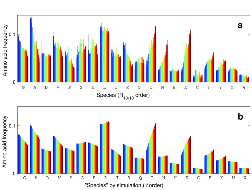
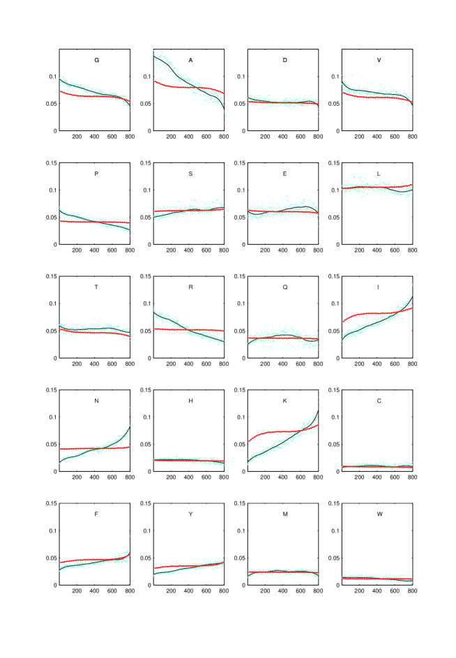
The chronology of amino acids to recruit into the genetic code from the earliest to the latest can be estimated as: G, A, D, V, P, S, E, L, T, R, Q, I, N, H, K, C, F, Y, M, W [13]. Let denote the amino acids in this chronological order. According to this amino acid chronology, some amino acids such as G and V recruited into the genetic code earlier than other amino acids such as H, Q and W. Let
denote the frequency of amino acid for the species in PEP () or in NCBI (), where denotes the total number of amino acid in all the protein sequences of species . If we sort the species properly, we can observe variation trends of amino acid frequencies when , roughly speaking, increases or decreases with .
We can introduce Late-early Ratio Orders to sort the species properly to observe variation trends of amino acid frequencies. In this class of orders, we can arrange the species by , namely the ratio of the average amino acid frequency of to the average amino acid frequency of , where are some later recruited amino acids and some earlier recruited amino acids. The Late-early Ratio Order is generally chronological in the evolution according to its definition. When the earlier recruited amino acids or later ones are given concretely, we can define
and obtain order. Similarly, we obtain order and order, where
and
order, order and order are some cases of Late-early Ratio Orders.
If we choose orders of species improperly, the variation trends of amino acid frequencies can not be observed. An improper choice is the Random Ratio Order. In this order, we arrange the species by Random Ratio Order , where the amino acids in numerator and denominator are chosen randomly among the amino acids. By this way, we can not observe variation trends of amino acid frequencies when vary with randomly. For instance, the species can be arranged by order, where
At last, we can introduce order to observe the variation trends of amino acid frequencies roughly. In this order, the species can be arranged from short to long by the average protein length of all the proteins in species. The order is independent of the choice of amino acids according to its definition.
2.1.2 General variation trends of amino acid frequencies
When sorting the species properly, we can obtain a set of variation trends for the amino acids. The variation trends are generally common for different proper orders of species, and the results of variation trends are also common either based on the data of species in PEP or based on the data of species in NCBI. So the general variation trends of amino acid frequencies are intrinsic properties of species.
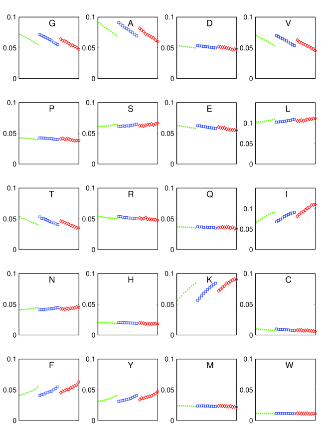
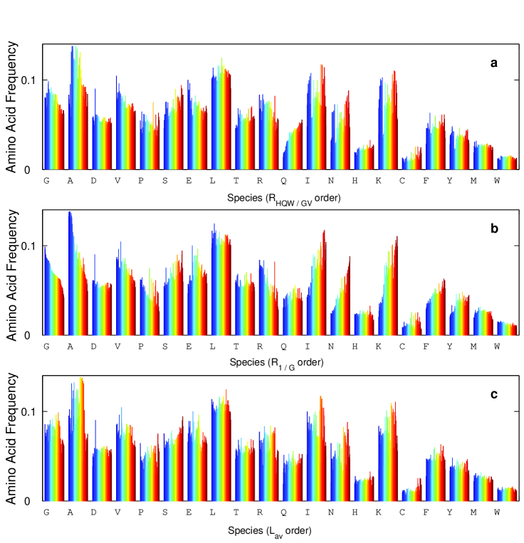
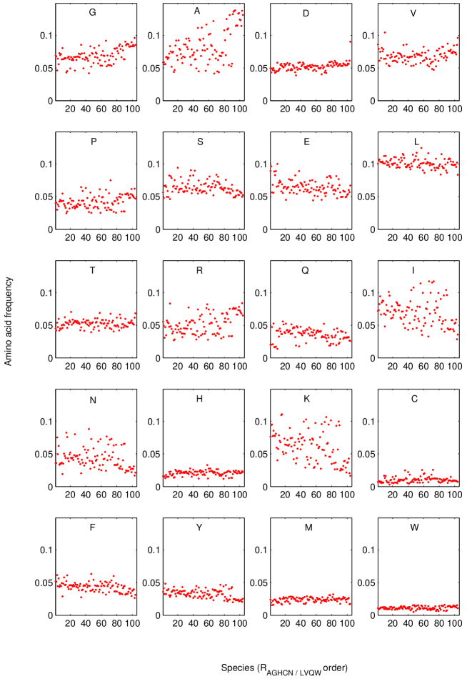
When sorting species by order, the amino acid frequencies based on species in PEP is in Fig. 1a, and the result based on species in NCBI is in Fig. S4. Both of the results are the same in variation trend for each of the amino acids. Roughly speaking, the frequencies of G, A, D, V, P, L, T, R, H, W tend to decrease, the frequencies of S, E, I, N, K, F, Y tend to increase, and the frequencies of Q, C, M tend to keep constant. The magnitudes of variations are different: frequencies of G, A, V, P, R decrease more rapidly than that of D, L, T, H, W, while frequencies of I, N, K, F, Y increase more rapidly than that of S, E. We found that the evolutionary trends of amino acids are related to the amino acid chronology [13]: most of the amino acids whose frequencies tend to decrease (or increase) are among the earlier (or later) recruited amino acids according to the amino acid chronology. The variation trends of amino acid frequencies are intrinsic properties of molecular evolution, which are irrelative to the choice of orders in sorting species. We can observe generally the same variation trends by order, order, order and order (Fig. 1a and Fig. S1). The variation trends are irrelative to the choice of amino acids, because we can also observe the same variation trends by order (Fig. S1c and Fig. S2). If sorting the species improperly, we can only observe completely random variation of amino acid frequencies (Fig. S3).
2.1.3 Fine structures of the variation of amino acid frequencies
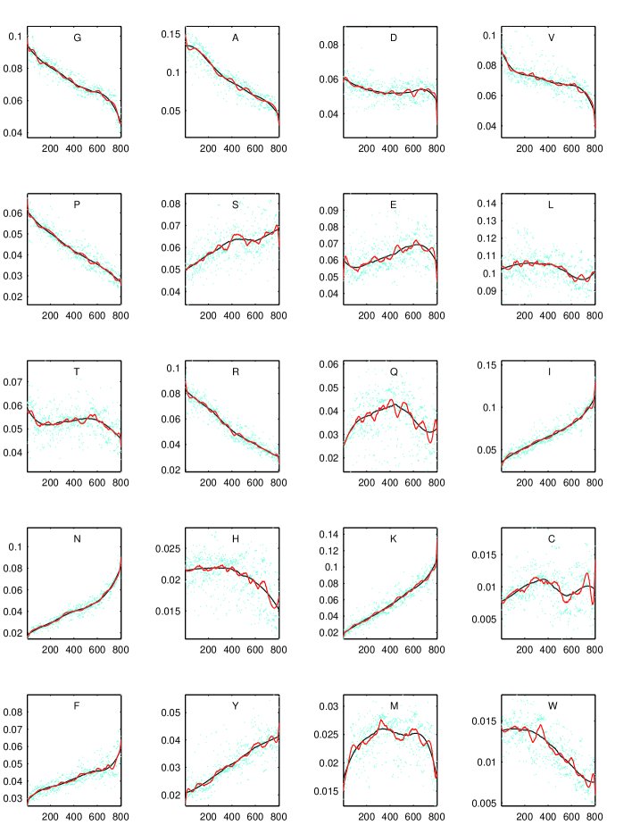
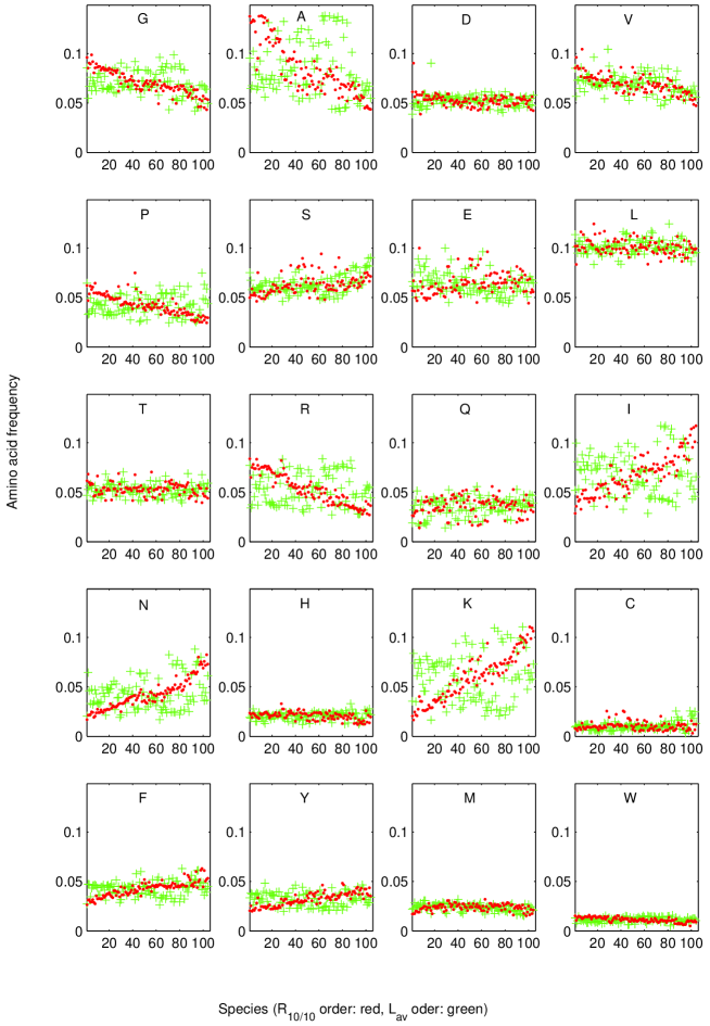
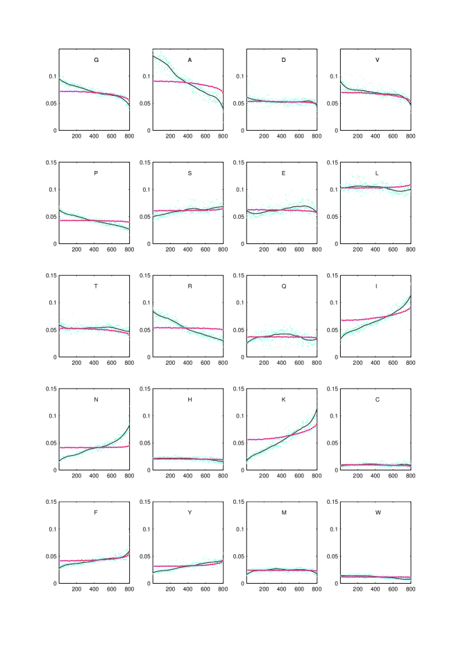
Furthermore, we can observe fine structures and superfine structures of the variation of amino acid frequencies because do not vary with linearly in general. We choose order in studying the variation of amino acid frequencies, which is an intrinsic order related to the molecular evolution. Roughly speaking, the species with lower (or higher) series number by order may appear earlier (or later) in the evolution according to the definition of . The details of variation of amino acid frequencies can be observed more obviously when studying the data of species in NCBI than studying the data of species in PEP. In the research, we obtained smoothed lines of the discrete dots (, ) for each amino acid according to Savitzky-Golay method [14]. The fine structures and superfine structures of the variation of amino acid frequencies can be observed explicitly according to the fluctuations in the smoothed lines.
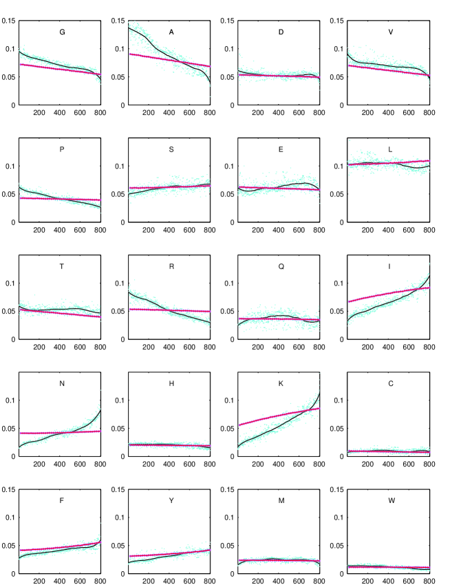
We prescribe the fine structures as the profiles of the variations of amino acid frequencies. The smoothed lines corresponding to fine structures can be obtained by certain greater spans according to Savitzky-Golay method (black lines in Fig. 2). The profiles of dots of the amino acid frequencies with respect to series numbers of species are S-shaped or inverse S-shaped in general. For examples, the profile of the dots (, ) is S-shaped and the profile of the dots (, ) is inverse S-shaped (see subplot V and subplot F in Fig. 2). Generally speaking, we can observe more steep variation trends at both ends. In the case for amino acids G, A, D, V, P, T, R whose variation trends are decreasing, the smoothed lines go down more quickly at both left and right, so we can observe S-shaped profiles approximately. In the case for amino acids S, I, N, K, F, Y whose variation trends are increasing, the smoothed lines go up more quickly at both ends, so we can observe inverse S-shaped profiles approximately. In the case for other amino acids Q, C, M, L, H, W, E, we can observe deformed S-shaped or waved profiles. Especially, we found that the trends are always well S-shaped or inverse S-shaped for most of the amino acids whose average amino acid frequencies are high, while the trends are deformed S-shaped for the amino acids whose average amino acid frequencies are low.
2.1.4 Superfine structures of the variation of amino acid frequencies
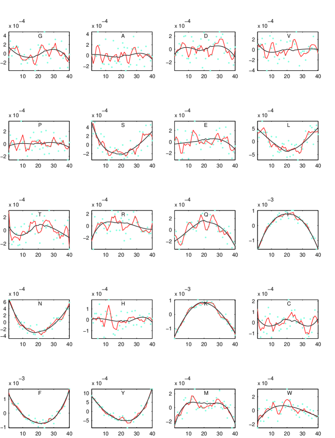
We prescribe the superfine structures as the fluctuations in the profiles of the variations of amino acid frequencies. The smoothed lines corresponding to superfine structures can be obtained by certain smaller spans according to Savitzky-Golay method (red lines in Fig. 2). We also sorted the species by order. We can show that the superfine structures do exist in the background of stochastic fluctuations. We can observe some obvious fluctuations in the smoothed lines. For examples, we can observe an obvious waved characteristic of fluctuations for amino acid W (for series number of species around in the subplot W in Fig. 2); we can observe a peak for amino acid S (for series number of species around in the subplot S in Fig. 2); we can observe two peaks for amino acid M (for series number of species around and in the subplot M in Fig. 2). Some obvious superfine structures can be observed in either the result based on NCBI (Fig. 2) or the result based on PEP (Fig. S2). We will explain the intrinsic property of the superfine structures by a model in section 2.2.3.
2.1.5 Variation trends of amino acid frequencies for three domains
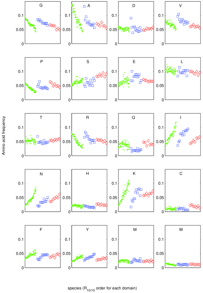
It is significant to compare the variation trends of amino acid frequencies for three domains (eubacteria, archaebacteria, and eukaryotes). The evolution trends of each of the amino acid frequencies are the same without exception for three domains (Fig. 4). But there are differences of the ranges of amino acid frequencies for three domains. The ranges of the variations of amino acid frequencies for eubacteria, roughly speaking, coincide with the ranges of the variations of amino acid frequencies for archaebacteria. There are, however, obvious differences between the ranges for archaebacteria and eukaryotes (Fig. 4). Namely, the initial amino acid frequencies for start series number of eukaryotes by order are less than (or greater than) initial amino acid frequencies for start series number of archaebacteria by order for amino acids whose trends decrease (or increase).
2.2 Theoretical results
2.2.1 General variation trends of amino acid frequencies
The variation trends of amino acid frequencies simulated by the model (Fig. 1b and red dots in Fig. S4) agree with the variation trends in experimental observations (Fig. 1a and celeste dots in Fig. S4) very well. The mechanism on the variation of amino acid frequencies is faithfully based on the genetic code multiplicity. The variation trends and magnitudes of amino acid frequencies are crucially related to the placements of amino acids in the genetic code multiplicity (Fig. S13). For examples, the amino acids F and Y occupy similar positions in the genetic code multiplicity, so the corresponding evolutionary trends and magnitudes accord with each other. The similar results are also valid for the amino acids G and A, for the amino acids P and H, for the amino acids R, D and E and for the amino acids L and S respectively (Fig. 1, S4 and S13). Hence, our result reveals that the underlying mechanism of the variation of amino acid frequencies in the contemporary species is determined by the evolution of genetic code.
The magnitudes of the variations of amino acid frequencies in the theoretical results are about half of the corresponding experimental observations. We did not add any more parameters in the model to boost the magnitudes of variation of amino acid frequencies in the model so as to obtain a better result concerning to the magnitudes, because we insisted on that the model is faithfully based on the genetic code multiplicity.
2.2.2 Fine structures of the variation of amino acid frequencies
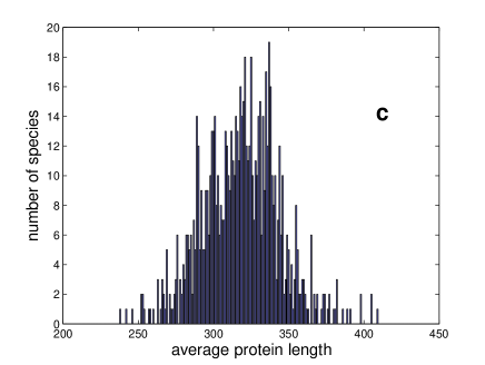
Up to a certain precision, the variation trends in theoretical results are linear for all the amino acids (red lines in Fig. S4). But the fine structures of the variation of amino acid frequencies obviously deviate from linear relationships in experimental observations (blank lines in Fig. S4 or blank lines in Fig. 2 for zoom in). According to the model, we can easily explain the S-shaped or inverse S-shaped profiles in fine structures of the variation of amino acid frequencies. The number of species in NCBI varies with average protein length as in Fig. S8c. This distribution indicates that the sample density of species in NCBI is not a constant when considering the relationship between amino acid frequencies and average protein length in Fig. 8. So series number does not vary linearly with the time in the evolution. Namely we only obtained less samples of species in the sections with small and big series numbers by order than in the sections with medium series numbers by order. As a result, we can observe more steep variation trends in the sections with small and big series numbers in the fine structures.
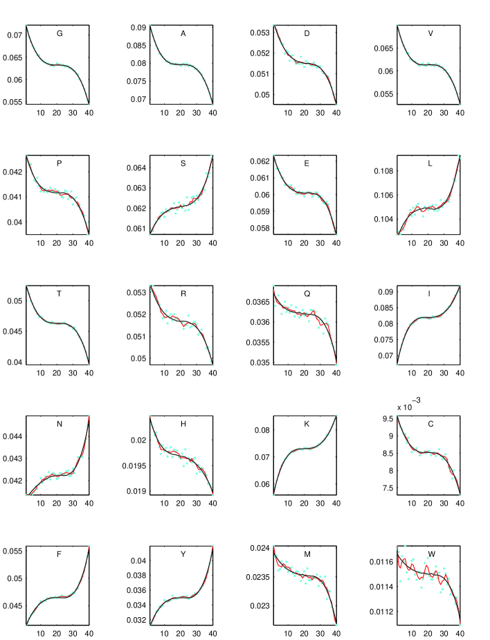
In the simulation in Fig. S4, we choose a linear relationship between parameter and series number of species , i.e., , without consideration of the variation of sample density. We introduce an simple function so as to obtain a similar relationship between number of species and parameter (Fig. S8a and S8b). Thus we obtained the fine structures of variations of amino acid frequencies (blank lines in Fig. 3, and Fig. S7 for zoom out). If we choose an improper function , which corresponds to unreasonable sample density, the simulated fine structures can not agree with the experimental observations in the sections with small series numbers (left ends of lines in Fig. S6). Therefore, we show that the reason to be either S-shaped profiles or inverse S-shaped profiles is trivially due to sample density of species in the databases.
The results in simulation (blank lines in subplots Q, C, M, L, H, W, E in Fig. 3) can not agree well with the deformed S-shaped experimental observations (blank lines in corresponding subplots in Fig. 2). If we can understand the evolution of genetic code in more details, the model may be improved and we may obtain a better result in the future.
2.2.3 Superfine structures of the variation of amino acid frequencies
We can observe the superfine structures of the variation of amino acid frequencies in theoretical results (red lines in Fig. 3). In the simulation, the amino acid frequencies are calculated based on sufficient numerous simulated protein sequences so as to avoid the random errors. All the fluctuations in Fig. 3 can recur in details if we run the program again. Therefore, the fluctuations of these smoothed lines are intrinsic properties of the variation of amino acid frequencies, which are determined by the genetic code multiplicity according to the mechanism of the model.
The simulation results indicate that the superfine structures in the experimental observations are also intrinsic properties (not just noises in observations) and should also be determined by the genetic code multiplicity. In this case, we can not compare the fluctuations between theoretical results and experimental observations in details. However, this heuristic conclusion may help us understand the evolution of genetic code in details by studying the fluctuations of superfine structures of the variation of amino acid frequencies.
It is possible for us to compare characteristics of superfine structures between theoretical results and experimental observations by the model. In the previous result in Fig. 2, we have introduced an artificial function . If we still let vary linearly with , i.e., , the results will only based on the genetic code multiplicity (red lines in Fig. S4). After subtracting the linear parts (in the sense of least squares), we can obtain the intrinsic fluctuations (not noises) of variation of amino acid frequencies (Fig. S5). We can also observe an obvious waved characteristic of fluctuations for amino acid W (subplot W in Fig. S5) and an double-peak characteristic for amino acid M (subplot M in Fig. S5), which might agree with the experimental observations.
2.2.4 Variation trends of amino acid frequencies for three domains
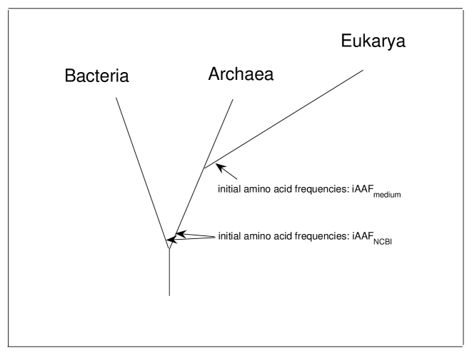
According to the phylogeny of three domains, Eukarya and Archaea separated later in the evolution, while Bacteria and the ancestor of both Eukarya and Archaea separated earlier in the evolution (Fig. S9) [15]. Hence, we can explain the differences of variation of amino acid frequencies for three domains in experimental observations in terms of the phylogeny of three domains. The unicellular organisms appeared earlier and eukaryotes appeared later in the history. We input some initial values of (Tab. 2) firstly in simulations of the evolution of amino acid frequencies for Bacteria and Archaea. Then, we input the medium amino acid frequencies of the previous step as initial amino acid frequencies to simulation the evolution of amino acid frequencies for Eukarya (Fig. S9). The simulation results (Fig. 5) agree with the experimental observations (Fig. 4) in general.
3 Variation of genetic code compositions
3.1 Experimental observations
It is well known that base compositions in genomes vary greatly, which are often referred as GC pressure or GA pressure in molecular evolution. There are delicate structures in the variation of genomic base compositions of contemporary species, which are discussed in details in Ref. [8].
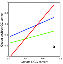
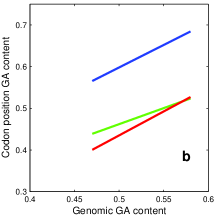
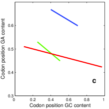
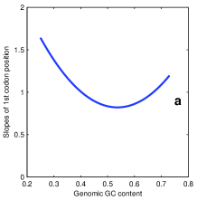
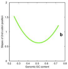
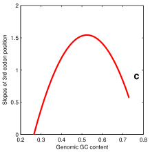
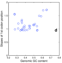
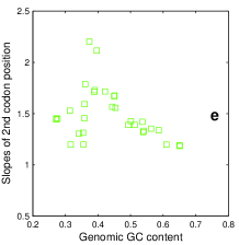
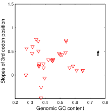
The precise correlations between genomic GC content (or genomic GA content) and the GC content (or GA content) at the first, second, or third codon positions can be observed obviously (Fig. 6a, 6b) [16] [8]. There are also correlations between codon position GC contents and codon position GA contents (Fig. 6c), or between genomic GC content and genomic GA content (Fig. 6d) [8]. Moreover, there are correlations between GC content of genes and codon position GC contents of genes in each genome, hence we can obtain three slopes of the corresponding correlations in first, second and third codon positions for a species [8]. The slopes corresponding to the three codon positions vary with genomic GC content respectively for contemporary species (Fig. S10a-S10c) [8].
3.2 Theoretical Results
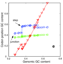
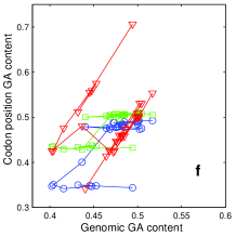
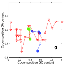
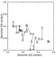
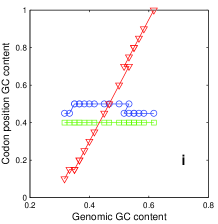
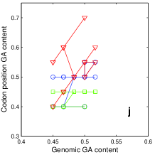
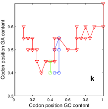
The mechanism of the evolution of genomic base compositions can also be explained by the same model based on genetic code multiplicity and codon chronology. The simulations of correlations of genomic base compositions and codon position base compositions (Fig. 6e-6h) agree with the experimental observations respectively (Fig. 6a-6d). It is noteworthy that there are many detailed agreements between simulations and experimental observations, which strongly confirm the validity of our simulations.
In Fig. 6e, we can observe a step in the middle of the line corresponding to the first codon position and a junction between lines corresponding to the first and second codon positions; these characters of step and junction can also be observed in the plots based on biological data [16][8][17]. The slope of the line corresponding to the third codon position is the deepest, because G and C occupy all the third positions of the earliest codons for amino acids, and A and U occupy all the third position of the latest codons for amino acids, but their compositions are about invariant for the first and second positions (Tab. 5-6). The lower limit and upper limit of the GC content for contemporary species also result from the base compositions in codon positions in a chronological list of codons. In Fig. 6f, the simulated slope corresponding to the third codon position is the greatest, which agrees with the experimental observation [8]. In Fig. 6g, the slopes and variation range in simulation agree with the experimental observation [8]. And in Fig. 6h, the deviation amplitude from the central declining line of the correlation between genomic GC content and genomic GA content is great, which agrees with the big standard error in Fig. 9-7 in Ref. [8]. At last, the simulations of the correlation between genomic GC content and the three slopes of correlations of GC content in genes (Fig. S10d-S10f) agree with the experimental observations [8] in principle. Thus, we show that the delicate structure in the correlations of genomic base compositions mainly comes from genetic code multiplicity and chronology (Fig. 6i-6l) [9][18].
4 Relationships among amino acid frequencies, genomic base compositions and average protein lengths
4.1 Experimental observations
4.1.1 Relationships between amino acid frequencies and genomic base compositions
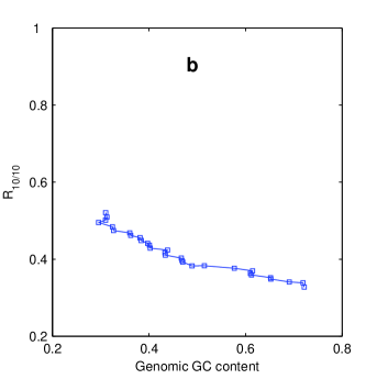
There is explicit relationship between amino acid frequencies and genomic base compositions. We observe that the genomic GC content decreases linearly with the ratio (Fig. 7a) [19][20]. Similar results are also valid for other Late-early Ratio Orders. So the genomic GC content and the amino acid frequencies are not independent variables when we discuss the evolutionary pressure in molecular evolution. It is often taken genomic GC content as the initial evolutionary pressure. If we can explain the relationships among amino acid frequencies, genomic base compositions and average protein lengths all together, it becomes not reasonable to take genomic GC content as the initial evolutionary pressure.
4.1.2 Relationships between amino acid frequencies and average protein lengths
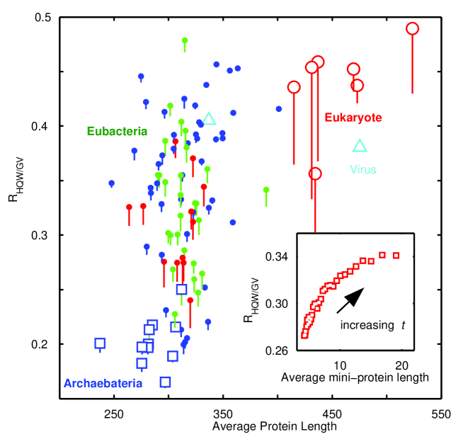
There is also correlation between the average protein length and the ratio (Fig. 8). The distribution of all species forms a bowed line in the plane, and the closely related species cluster together in the plane (Fig. 8). Roughly speaking, the average protein length becomes longer and longer in the evolution and there will be more and more opportunities for later recruited amino acid to appear in the protein sequences. Similar results are also valid for other Late-early Ratio Orders. We choose in order that the distribution of archaebacteria can be separated from the distribution of bacteria. We also noticed that the species with larger genome size locate in the midstream of the evolutionary flow. So this bowed distribution can be interpreted as an evolutionary flow. And more advanced prokaryotes with larger genome sizes always locate in the midstream of this evolutionary flow.
4.2 Theoretical Results
4.2.1 Relationships between amino acid frequencies and genomic base compositions
According to the simulation, we found that the genetic code multiplicity can influence both amino acid frequencies and genomic GC content. So the evolutionary pressure in the overall molecular evolution originated in the genetic code evolution. The evolutionary pressure influences the amino acid frequencies, genomic base composition and the average protein length in proteome all together.
When the parameter increases, there will be more and more late amino acids to join the protein sequences, so the ratio will also increase, but the genomic GC content will decrease according to the codon chronology. Thus we can explain that the ratio increases when the genomic GC content decrease (Fig. 7b). The variation range of in simulation (Fig. 7b) is less than the variation range of in experimental observation (Fig. 7a), which is due to that the magnitudes of variations of amino acid frequencies are insufficient in simulations by the model.
The variation of amino acid frequencies also influenced the genomic base compositions. For example, the total numbers of bases G and C are equal to in all stages for the second codon position and almost constant ( to ) for the first codon position (Tab. 6 and Fig 6i). In the simulation result, however, the GC content at the first and second codon position obviously decrease from right to left (corresponding to parameter increases from to ) (Fig. 6e). In the simulation, the probabilities for the late recruited amino acids (with less bases G and C in their codons, see Tab. 5) to join the proteins will increase when the parameter increases, therefore the GC content at the first and second codon positions decrease from right to left in Fig. 6e. Thus, we can explain the slopes of the correlations between genomic GC content and the GC content at codon positions in Fig. 6a.
4.2.2 Relationships between amino acid frequencies and average protein lengths
The relationship between amino acid frequencies and average protein length can be explained by the model. The distribution of species in the plane can be simulated by our model (Fig. 8, Embedded). The bending direction of the simulated evolutionary flow agrees with the evolutionary flow in experimental observation. According to the simulation by the model, the bending direction sensitively relates to the genetic code multiplicity. If we vary the substitution rules a little, the bending curve may disappear in the result by simulation and we can only obtain a linear relationship between and . So such a detail agreement between theoretical result and experimental observation verifies the validity of the referred genetic code multiplicity in the model (Fig. S13 and Ref. [9]).
5 Genetic code evolution as an initial driving force for molecular evolution
5.1 Timing the mechanism of the variation of amino acid frequencies
The estimation of the time when the variation of amino acid frequencies appeared firstly will help us seek the mechanism that determines the variation of amino acid frequencies of contemporary species. We can explain that the variation of amino acid frequencies formed before the stage when three domains began to branch.
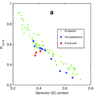
Firstly, we explain the incorrelation between the variation of amino acid frequencies in our observations and the gain-loss of amino acids in modern time. The trend of amino acid gain and loss in protein evolution has been reported in Ref. [10]. There is a debate on the mechanism of the variation of amino acid frequencies [21]. There is a set of data of gain and loss for amino acids in Ref. [10] according to the protein evolution in modern time (Tab. 1). We can also obtain a set of data of variation trends for amino acids according to Fig. 1a by least squares (Tab. 1). The correlation efficient between gain-loss and variation trends is , which means that the variation trends are incorrelated with the gain and loss of amino acids in modern time. If it is true, we can infer that the mechanism of the variation of amino acid frequencies should appeared in early period.
The variation of amino acid frequencies for three domains may help us time the mechanism of the variation of amino acid frequencies. The evolutionary trends of amino acid frequencies are the same for three domains (Fig. 4). And we have explained the differences of amino acid frequencies for three domains according to the phylogeny of three domains in section 2.2.4. These results indicate that the mechanism of the variation of amino acid frequencies should originate in the period before the separation between Bacteria and the ancestor of Archaea and Eukarya.
5.2 Initial driving force for molecular evolution
The variations of amino acid frequencies and genomic base compositions can be explained in a unified theoretical framework based on genetic code evolution. All the theoretical results in section 2-4 are based on one model, whose core is the genetic code multiplicity and chronology. The simulations by the model agree with the experimental observations not only in variation trends but also in many detailed characteristics. So there is close relationship between the variation of amino acid frequencies and genomic base compositions of contemporary species and the genetic code evolution in the primordial period. We believe that () the pattern of the variation of the compositions of protein and DNA formed and fixed in the period when the genetic code evolved; () the magnitudes of the evolutionary trends have been amplifying ever since the genetic code had established. Thus, we conjecture that the genetic code evolution is an initial driving force for molecular evolution.
5.3 Cracking the genetic code evolution
If our conjecture is reasonable, we found a new method to crack the genetic code evolution in primordial time by studying the variation of amino acid frequencies and genomic base compositions of contemporary species. Especially, there are some detailed disagreements between theoretical results and experimental observations. For instance, we can not compare the superfine structures in details between theoretical results and experimental observations. The improvement in understanding the variation of amino acid frequencies and genomic base compositions may lead us to crack the genetic code evolution.
6 The model
6.1 Outline of the model
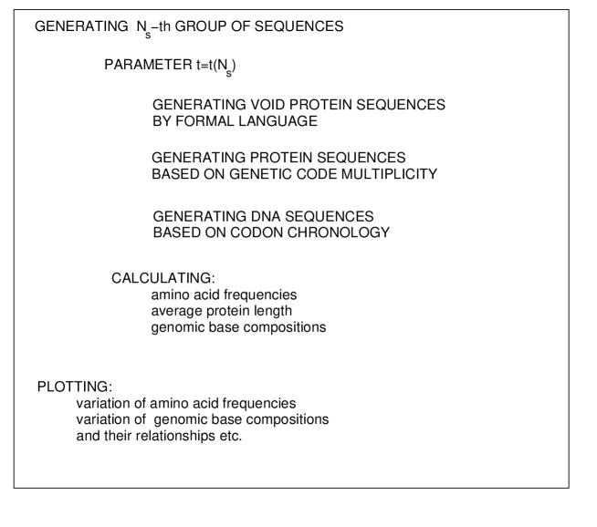
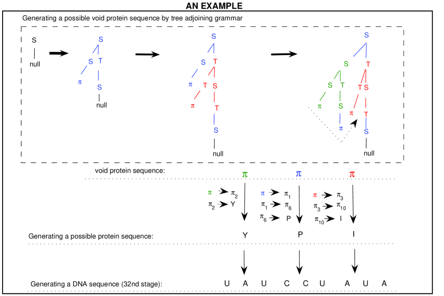
We proposed a model based on the evolution of genetic code to explain the variations of amino acid frequencies and base compositions in species. The model mainly consists of three parts: () generating void protein sequences by formal language; () generating protein sequences based on genetic code multiplicity; and () generating DNA sequences based on codon chronology (Fig. S11).
The genetic code multiplicity (Fig. 13) is the core in simulation of variation of amino acid frequencies. The genetic code chronology (Tab. 5) is the core in simulation of variation of genomic base compositions. This is an elaborate model and there is only one adjustable parameter , which indicates the time of the evolution and plays central roles in simulations of the variations of amino acid frequencies and base compositions.
6.2 Simulation of the variation of amino acid frequencies
6.2.1 Generation of void protein sequences by formal language
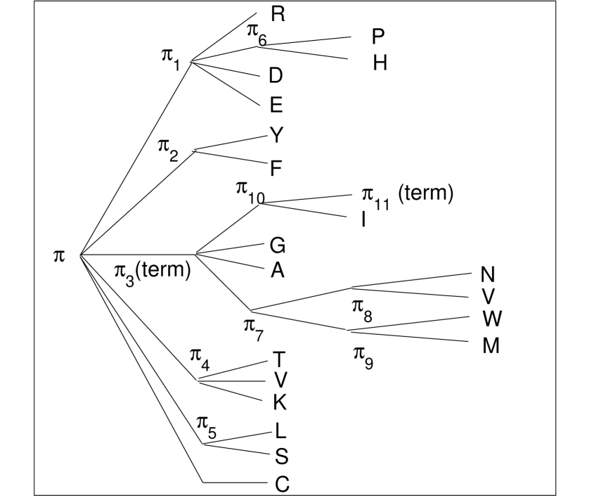
There are two steps in generation of protein sequences in the model: (1) generating void protein sequences according to tree adjoining grammars in Fig. S12 [22]; (2) the leaf in the tree adjoining grammar will be substituted by amino acids based on the genetic code multiplicity in Ref. [9] (Fig. S13 and Tab. 3), where the amino acid chronology has been considered according to Ref. [13] and the probabilities for substitutions are determined by in Tab. 2.
There are no rigorous restrictions in choosing grammar rules of the formal language, because they do not essentially determine the variation trends of amino acid frequencies in our final results. In the model, we choose tree adjoining grammar to generate void protein sequences. There are one initial tree and two associate trees in the grammar rules, where and are inner nodes and is leaf (Fig. S12). We start from the initial tree when generating a void protein sequence. Then the inner nodes or can be substituted by the corresponding associate trees (see the example in Fig. S14). The void protein sequence consists of the leaves around the final tree.
We set a parameter in the model as the probability of the substitution of inner nodes. The length of a sequence may increase if an inner node has been substituted by the corresponding auxiliary tree (with probability ) or keep constant if the node has not been substituted (with probability ). The void protein sequences consist of void character , which will be substituted by amino acids in the next step. When the parameter is fixed, we can generate a group of void sequences with certain length distribution. In the model, the void protein sequences increase only several units in length in each principal cycle of the program. The number of cycles in the program is constant in the model. We can obtain longer void protein sequences after running more principal cycles. The average increment of protein length in one principal cycle varies with respect to parameter . When increases, there will be more probability to generate longer void protein sequences in each principal cycle.
6.2.2 Fill in the protein sequences based on genetic code multiplicity
In the second step, the void character in the void protein sequences will be substituted by amino acids by calling a subprogram. The rules of substitutions in the subprogram are based rigorously on the genetic code multiplicity (Fig. S13, Tab. 3). Namely, may be substituted by either of , , , , or amino acid at first level of substitution; may be substituted by either of , , or at second level of substitution, and so on; may be substituted by either of or at third level of substitution, and so on (Fig. S13, Tab. 3). The depth of substitutions of the genetic code multiplicity tree is four levels in maximum, namely from to , , or (Fig. S13, Tab. 3). The process of substitution of will not finish until is substituted by one of the amino acids eventually. Thus, the protein sequences consisting of amino acids have been generated.
The probabilities for all the possible substitutions of each node in the genetic code multiplicity tree (Fig. S13, Tab. 3) are constant parameters in the model according to the average amino acid frequencies of contemporary species. The initial amino acid frequencies (iAAF) at the beginning of each cycle in the program are input by the average amino acid frequencies of species in PEP () or NCBI () (Tab. 2):
We choose the average amino acid frequencies as the initial amino acid frequencies in order that the average amino acid frequencies in the simulation results agree with the average amino acid frequencies in observation. But these constant parameters do not influence the variation trends in the simulations. The corresponding probabilities for amino acids can be calculated as followings:
where (namely will be substituted by and with the equal probability in Fig. S13). According to Tab. 3, all the probabilities of substitution between two connected nodes in Fig. S13 can be calculated by the initial amino acid frequencies. In the substitution of by , for instance, the probability is ; while the probability of substitution of by is (Tab. 2).
6.2.3 Calculation of amino acid frequencies and their variation trends
When the parameter is fixed, we can generate sufficient numerous protein sequences so that the amino acid frequency for each of the amino acids goes to a certain constant value. Then, the amino acid frequencies vary with parameter .
We can study the evolution of amino acid frequencies by adjusting the parameter from to . We observed that the amino acid frequency for each amino acid may increase or decrease when increases. For the initial parameter , we input as initial values of amino acid frequencies. We chose sample species and obtained sets of amino acid frequencies by the model. Hence, we can obtain the variation trends of amino acid frequencies in the simulation. We found that the variation trends of amino acid frequencies are irrelative to the initial values of the amino acid frequencies, which are determined by the genetic code multiplicity.
6.2.4 The mechanism of the variation of amino acid frequencies in the simulation
According to the simulation by the model, the genetic code multiplicity plays central role in the evolution of amino acid frequencies. It should take more steps of substitutions to replace in the void protein sequences by a late recruited amino acid. The placements of amino acids in the genetic code multiplicity tree essentially influence the variation of amino acid frequencies in the simulation. When we generate shorter protein sequences, the late recruited amino acids have less opportunities to join the protein sequences. When the parameter increases, the increment of protein length in one principal cycle also becomes greater than before. Hence, there will be more opportunities for the late recruited amino acids to join the protein sequences. So the amino acid frequencies will vary with the parameter . The only continuous variable in the model can be interpreted as the time in the evolution. The other constant parameters and the grammar rules do not essentially influence the variation trends. And there are no other parameters in the model to deliberately influence certain amino acid frequencies or genomic base compositions.
6.3 Simulation of the variation of genomic base compositions
6.3.1 Codon chronology
The codon chronology can be reconstructed based on the amino acid chronology and the primacy of thermostability and complementarity (Tab. 4) [13][18][23][24]. The result of codon chronology in Tab. 4 is almost the same as the chronology in Ref. [23], but amino acid chronology in the first line of Tab. 4 in our calculation is replaced by a new amino acid chronology obtained by the same authors in Ref. [13] that was published later than Ref. [23]. In our results, the amino acids are sorted chronologically in the first line in Tab. 4. The pairs of complementary codons are sorted chronologically from top to bottom in Tab. 4, which correspond to the above amino acid chronology and form a lower triangle in Tab. 4.
The codon chronology in Tab. 4 can explain the relationship between GC content and codon position GC content very well. But the declining relationship between genomic GC content and genomic GA content in experimental observations (Fig. 6d) must not be achieved by the codon chronology in Tab. 4 in principle because of the rigorous restriction of codon complementarity. We have to modify the chronology slightly in sacrifice of the codon complementarity so that the relationship between genomic GC content and genomic GA content in experimental observation (Fig. 6d) can be simulated by the model. We only rearranged the codon chronology for amino acids S and R and obtained a modified codon chronology (Tab. 5). Namely, we moved the positions of codons AGC and AGU earlier in Tab. 5 than in Tab. 4 for amino acid S; and we moved the positions of codons AGG and AGA earlier in Tab. 5 than in Tab. 4 for amino acid R.
According to the codon chronology in Tab. 5, there are stages in the evolution of genetic codes. For each stage, there is a definitive correspondence between a codon and a certain amino acid. For each stage, therefore, we can count the total numbers of bases G, C, A or T for all the amino acids in the first, second or third codon positions respectively according to Tab. 5 (Tab. 6). And we also obtained the total number of G and C and the total number of G and A in the first, second and third codon positions respectively as well as the total numbers of G and C or G and A in all the three codon positions (Tab. 6). The results in Tab. 6 partially indicate the variation trends of genomic base compositions. And we can plot the relationships in Fig. 6i-6l according to Tab. 6.
6.3.2 Generation of DNA sequences according to codon chronology
There is a one to one relationship between amino acids and a codon at each of the stages according to the codon chronology in Tab. 5. We separated the section [, ] equally into subsections so that each value of parameter is in one of these subsections. Thus, the amino acids in the protein sequences generated in the second part of the model can be replaced by corresponding codons at certain stages. So there is also a one to one correspondence between protein sequences and DNA sequences at each stage. Thus a group of DNA sequences can be obtained in the model as soon as the protein sequences have been generated, which is based on both the genetic code multiplicity and the codon chronology.
6.3.3 Calculation of genomic base compositions and their variation trends
For a fixed value of parameter , which corresponds to a certain stage, we can obtain numerous DNA sequences. Then we can calculate the compositions of bases G, C, A, T. At last, we can obtain GC content or GA content at certain codon positions and the total GC content or GA content in all the DNA sequences. When the parameter varies, we can study the evolution of genomic base compositions or base compositions at certain codon positions.
6.3.4 The mechanism of the variation of genomic base compositions in the simulation
According to the simulation in the model, the variation of base compositions in contemporary species can be explained by the codon chronology, genetic code multiplicity and amino acid chronology together. For instance, we can explain the relationship between genomic GC content and GC content at the first, second and third codon positions. The plot of the relationship between total GC numbers and GC number at certain codon positions in Fig. 6i is approximate the same as the corresponding experimental observation in Fig. 6a. The upper limit (about ) and lower limit (about ) of genomic GC content are due to the abundance of G and C in the earliest codons and lack of G and C in the latest codons in Tab. 5. The characteristic of “step” at the middle for the third codon position in experimental observation is due to the leap of numbers of G and C at third codon position in Tab. 6. There are always G and C at the second codon position in Tab. 6, so there is no step for the second codon position in experimental observation. The simulation of GC content for each codon position increases with genomic GC content (Fig. 5e), which agrees with the experimental observation (Fig. 5a). When increases, there will be less opportunities for bases G and C to join the DNA sequences. The other relationships in Fig. 6 can also be explained similarly.
6.4 Simulation of relationships among amino acid frequencies, genomic base compositions and average protein lengths
6.4.1 Relationships between amino acid frequencies and genomic base compositions
When the parameter is fixed, both of a group of proteins and a group of corresponding DNA sequences can be generated together by the model. Subsequently, both of the amino acid frequencies and genomic GC content can be calculated. Thus we can explain that the ratio increases when the genomic GC content decrease (Fig. 7a).
6.4.2 Relationships between amino acid frequencies and average protein lengths
When the parameter is fixed, a group of proteins can be generated by the model. So both the amino acid frequencies and average protein length can be calculated together. When varies, we can obtain the relationship between and average protein length (Fig. 8, Embedded), which agrees with the experimental observation very well (Fig. 8). We obtained a bended curve for the relationship between and , whose bending direction is upward (Fig. 8, Embedded). The bending direction is also the same for relationships between and in simulation.
7 Conclusion
The variation of amino acid frequencies and the variation of genomic base compositions can be explained in a unified framework based on genetic code evolution. According to the model, we show that the genetic code multiplicity plays central roles in explanation of the variation of amino acid frequencies of contemporary species. The theoretical results agree with the experimental observations not only in the variation trends but also in the fine structures or superfine structures. And we also show that the codon chronology plays central roles in explanation of the variation of genomic base compositions of contemporary species. Our results agree with the experimental observations in many details, such as S-shaped or inverse S-shaped profiles in Fig. 2, differences of ranges of amino acid frequencies between Archaea and Eukarya in Fig. 4, characteristics of step and junction in Fig. 6e, bending direction in Fig. 8 etc, which confirm the validity of our theory. We also explained that the mechanism to determine the variation of amino acid frequencies originated before the stage when three domains began to branch. So we conclude that the evolution of genetic code is the initial driving force in molecular evolution, and the evolution of genetic code in the primordial period determines the variations of amino acid frequencies and genomic base compositions of contemporary species.
Acknowledgments
We thank Hefeng Wang for valuable discussions. Supported by NSF of China Grant No. of 10374075.
References
- [1] Knight R. D., and Landweber L. F. The early evolution of the genetic code. Cell 101, 569-572 (2000).
- [2] Szathmáry, E. Why are there four letters in the genetic alphabet? Nature Rev. Genetics 4, 995-1001, (2003).
- [3] Crick, F. H. C. The Origin of the Genetic Code. J. Mol. Biol. 38, 376-379 (1968).
- [4] Osawa, S. et al., Recent evidence for evolution of the genetic code. Microbiol. Rev. 56 229-264 (1992).
- [5] Trifonov, E. N. et al., Distinct stages of protein evolution as suggested by protein sequence analysis. J. Mol. Evol. 53, 394-401 (2001).
- [6] Carter, P., Liu, J. and Rost, B. PEP: Predictions for Entire Proteomes. Nucleic Acids Research 31, 410-413 (2003).
- [7] Haft D. H., Selengut J. D., Brinkac L. M., Zafar N., and White O. Genome Properties: a system for the investigation of prokaryotic genetic content for microbiology, genome annotation and comparative genomics. Bioinformatics 21, 293-306 (2005).
- [8] Forsdyke, D. R., Evolutionary Bioinformatics (Springer, New York, 2006).
- [9] Hornos, J. E. M., and Hornos, Y. M. M., Algebraic Model for the Evolution of the Genetic Code. Phy. Rev. Lett. 71, 4401-4404 (1993).
- [10] Jordan, I. K. et al. A univeral trend of amino acid gain and loss in protein evolution. Nature 433, 633-638, (2005).
- [11] Rost, B. Did evolution leap to create the protein universe? Curr. Opin. Stru. Biol. 12, 409-416 (2002).
- [12] Liu, J.-F. and Rost, B. Comparing function and structure between entire proteomes. Protein Sci. 10, 1970-1979 (2001).
- [13] Trifonov, E. N. The triplet code from first principle. J. Biomol. Struct. Dyn. 22, 1-11 (2004)
- [14] Savitzky, A. and Golay, M. J. E. Smoothing and differentiation of data. Anal. Chem. 36, 1627-1639 (1964).
- [15] Woese, C. R., Kandler, O. and Wheelis, M. L. Towards a natural system of organisms: Proposal for the domains Archaea, Bacteria, and Eucarya. Proc. Natl. Acad. Sci. USA 87, 4576-4579 (1990).
- [16] Muto A., and Osawa S. The guanine and cytosine content of genomic DNA and bacterial evolution. Proc. Natl. Acad. Sci. USA 84, 166-169 (1987).
- [17] Gorban, A. et al., Codon usage trajectories and 7-cluster structure of 143 complete bacterial genomic sequences. Physica A 353, 365-387 (2005).
- [18] Trifonov, E. N., Consensus temporal order of amino acids and evolution of the triplet code. Gene 261, 139-151 (2000). 53, 394-401 (2001).
- [19] Sueoka N. Correlation between base composition of deoxyribonucleic acid and amino acid composition of protein. Proc. Natl. Acad. Sci. USA 47, 1141-1149 (1961).
- [20] Gu X., Hewett-Emmett D., and Li W.-H. Directional mutational pressure affects the amino acid composition and hydrophobicity of proteins in bacteria. Genetica 103, 383-391 (1998).
- [21] Hurst, L. D., Feil E. J., Rocha E. P. C. Causes of trends in amino-acid gain and loss. Nature 442, E11-E12 (2006).
- [22] Joshi, A. K. and Schabes, Y., in Handbook of Formal Lan- guages, eds G. Rozenberg and A. Salomma, pp.69-214 (Springer, Heidelberg, 1997).
- [23] Trifonov, E. N., Kirzhner, A., Kirzhner, V. M., and Berezovsky, I. N. Distinct stages of protein evolution as suggested by protein sequence analysis. J. Mol. Evol. 53, 394-401 (2001).
- [24] Eigen, M., and Schuster, P., The hypercycle. A principle of natural self-organization. Part C: The realistic hypercycle. Naturwissenschaften 65 341-369 (1978). *E-mail: dirson@mail.xjtu.edu.cn


SUPPLEMENTARY FIGURES AND TABLES
Guide to figures and tables
Group I: Fig. 1, Fig. S1-S4, Tab. 1. Variation trends of amino acid frequencies.
Group II: Fig. 2-3, Fig. S5-S8. Fine structures and superfine structures of the variation of amino acid frequencies.
Group III: Fig. 4-5, Fig. S9. Variation of amino acid frequencies for three domains.
Group IV: Fig. 6, Fig. S10. Variation of genomic base compositions.
Group V: Fig. 7-8. Relationship between amino acid frequencies and genomic base compositions, and relationship between amino acid frequencies and average protein length
Group VI: Fig. S11-S14, Tab. 2-6. The model based on genetic code multiplicity and codon chronology.
SUPPLEMENTARY FIGURES S1-S14

SUPPLEMENTARY TABLES 1-6
| G | A | D | V | P | S | E | L | T | R | Q | I | N | H | K | C | F | Y | M | W | |
| Evol. trend () | -354 | -765 | -62.9 | -245 | -292 | 128 | 77.0 | -61.0 | -42.9 | -475 | 9.95 | 590 | 490 | -57.0 | 734 | -14.7 | 214 | 187 | -1.27 | -59.5 |
| Gain-loss () | -63 | -239 | -39 | 98 | -139 | 167 | -137 | -17 | 91 | 38 | 20 | 89 | 73 | 73 | -65 | 67 | 42 | -5 | 88 | 2 |
| () | 692 | 831 | 524 | 674 | 489 | 703 | 647 | 991 | 537 | 559 | 394 | 577 | 400 | 226 | 555 | 141 | 404 | 299 | 238 | 119 |
|---|---|---|---|---|---|---|---|---|---|---|---|---|---|---|---|---|---|---|---|---|
| () | 721 | 906 | 536 | 698 | 427 | 607 | 624 | 1025 | 527 | 537 | 366 | 672 | 413 | 204 | 560 | 97 | 414 | 312 | 238 | 116 |
| () | 639 | 804 | 516 | 619 | 410 | 622 | 597 | 1051 | 464 | 520 | 365 | 811 | 421 | 195 | 721 | 84 | 464 | 348 | 237 | 114 |
| [1] | |||
| G | A | D | V | P | S | E | L | T | R | Q | I | N | H | K | C | F | Y | M | W | (stop) | (S) | (L) | (R) | |
| 1 | GGC | GCC | ||||||||||||||||||||||
| 2 | GAC | GUC | ||||||||||||||||||||||
| 3 | GGG | CCC | ||||||||||||||||||||||
| 4 | GGA | UCC | ||||||||||||||||||||||
| 5 | GAG | CUC | ||||||||||||||||||||||
| 6 | GGU | ACC | ||||||||||||||||||||||
| 7 | GCG | CGC | ||||||||||||||||||||||
| 8 | CCG | CGG | ||||||||||||||||||||||
| 9 | UCG | CGA | ||||||||||||||||||||||
| 10 | ACG | CGU | ||||||||||||||||||||||
| 11 | CUG | CAG | ||||||||||||||||||||||
| 12 | GAU | AUC | ||||||||||||||||||||||
| 13 | GUU | AAC | ||||||||||||||||||||||
| 14 | AUU | AAU | ||||||||||||||||||||||
| 15 | GUG | CAC | ||||||||||||||||||||||
| 16 | CUU | AAG | ||||||||||||||||||||||
| 17 | GCA | UGC | ||||||||||||||||||||||
| 18 | ACA | UGU | ||||||||||||||||||||||
| 19 | GAA | UUC | ||||||||||||||||||||||
| 20 | AAA | UUU | ||||||||||||||||||||||
| 21 | GUA | UAC | ||||||||||||||||||||||
| 22 | AUA | UAU | ||||||||||||||||||||||
| 23 | CAU | AUG | ||||||||||||||||||||||
| 24 | CCA | UGG | ||||||||||||||||||||||
| 25 | CUA | UAG | ||||||||||||||||||||||
| 26 | UCA | UGA | ||||||||||||||||||||||
| 27 | GCU | AGC | ||||||||||||||||||||||
| 28 | ACU | AGU | ||||||||||||||||||||||
| 29 | CAA | UUG | ||||||||||||||||||||||
| 30 | UAA | UUA | ||||||||||||||||||||||
| 31 | CCU | AGG | ||||||||||||||||||||||
| 32 | UCU | AGA |
| G | A | D | V | P | S∗ | E | L | T | R∗ | Q | I | N | H | K | C | F | Y | M | W | |
|---|---|---|---|---|---|---|---|---|---|---|---|---|---|---|---|---|---|---|---|---|
| 1 | GGC | GCC | GAC | GUC | CCC | AGC | GAG | CUC | ACC | AGG | CAG | AUC | AAC | CAC | AAG | UGC | UUC | UAC | AUG | UGG |
| 2 | GGG | GCG | GAC | GUC | CCC | AGC | GAG | CUC | ACC | AGG | CAG | AUC | AAC | CAC | AAG | UGC | UUC | UAC | AUG | UGG |
| 3 | GGG | GCG | GAU | GUU | CCC | AGC | GAG | CUC | ACC | AGG | CAG | AUC | AAC | CAC | AAG | UGC | UUC | UAC | AUG | UGG |
| 4 | GGA | GCG | GAU | GUU | CCG | AGU | GAG | CUC | ACC | AGG | CAG | AUC | AAC | CAC | AAG | UGC | UUC | UAC | AUG | UGG |
| 5 | GGU | GCG | GAU | GUU | CCG | AGU | GAG | CUC | ACC | AGG | CAG | AUC | AAC | CAC | AAG | UGC | UUC | UAC | AUG | UGG |
| 6 | GGU | GCG | GAU | GUU | CCG | AGU | GAA | CUG | ACC | AGG | CAG | AUC | AAC | CAC | AAG | UGC | UUC | UAC | AUG | UGG |
| 7 | GGU | GCG | GAU | GUU | CCG | AGU | GAA | CUG | ACG | AGG | CAG | AUC | AAC | CAC | AAG | UGC | UUC | UAC | AUG | UGG |
| 8 | GGU | GCA | GAU | GUU | CCG | AGU | GAA | CUG | ACG | AGA | CAG | AUC | AAC | CAC | AAG | UGC | UUC | UAC | AUG | UGG |
| 9 | GGU | GCA | GAU | GUU | CCA | AGU | GAA | CUG | ACG | CGC | CAG | AUC | AAC | CAC | AAG | UGC | UUC | UAC | AUG | UGG |
| 10 | GGU | GCA | GAU | GUU | CCA | UCC | GAA | CUG | ACG | CGG | CAG | AUC | AAC | CAC | AAG | UGC | UUC | UAC | AUG | UGG |
| 11 | GGU | GCA | GAU | GUU | CCA | UCC | GAA | CUG | ACA | CGA | CAG | AUC | AAC | CAC | AAG | UGC | UUC | UAC | AUG | UGG |
| 12 | GGU | GCA | GAU | GUU | CCA | UCC | GAA | CUU | ACA | CGA | CAA | AUC | AAC | CAC | AAG | UGC | UUC | UAC | AUG | UGG |
| 13 | GGU | GCA | GAU | GUU | CCA | UCC | GAA | CUU | ACA | CGA | CAA | AUU | AAC | CAC | AAG | UGC | UUC | UAC | AUG | UGG |
| 14 | GGU | GCA | GAU | GUG | CCA | UCC | GAA | CUU | ACA | CGA | CAA | AUU | AAU | CAC | AAG | UGC | UUC | UAC | AUG | UGG |
| 15 | GGU | GCA | GAU | GUG | CCA | UCC | GAA | CUU | ACA | CGA | CAA | AUA | AAU | CAC | AAG | UGC | UUC | UAC | AUG | UGG |
| 16 | GGU | GCA | GAU | GUA | CCA | UCC | GAA | CUU | ACA | CGA | CAA | AUA | AAU | CAU | AAG | UGC | UUC | UAC | AUG | UGG |
| 17 | GGU | GCA | GAU | GUA | CCA | UCC | GAA | CUA | ACA | CGA | CAA | AUA | AAU | CAU | AAA | UGC | UUC | UAC | AUG | UGG |
| 18 | GGU | GCU | GAU | GUA | CCA | UCC | GAA | CUA | ACA | CGA | CAA | AUA | AAU | CAU | AAA | UGU | UUC | UAC | AUG | UGG |
| 19 | GGU | GCU | GAU | GUA | CCA | UCC | GAA | CUA | ACU | CGA | CAA | AUA | AAU | CAU | AAA | UGU | UUC | UAC | AUG | UGG |
| 20 | GGU | GCU | GAU | GUA | CCA | UCC | GAA | CUA | ACU | CGA | CAA | AUA | AAU | CAU | AAA | UGU | UUU | UAC | AUG | UGG |
| 21 | GGU | GCU | GAU | GUA | CCA | UCC | GAA | CUA | ACU | CGA | CAA | AUA | AAU | CAU | AAA | UGU | UUU | UAC | AUG | UGG |
| 22 | GGU | GCU | GAU | GUA | CCA | UCC | GAA | CUA | ACU | CGA | CAA | AUA | AAU | CAU | AAA | UGU | UUU | UAU | AUG | UGG |
| 23 | GGU | GCU | GAU | GUA | CCA | UCC | GAA | CUA | ACU | CGA | CAA | AUA | AAU | CAU | AAA | UGU | UUU | UAU | AUG | UGG |
| 24 | GGU | GCU | GAU | GUA | CCA | UCC | GAA | CUA | ACU | CGA | CAA | AUA | AAU | CAU | AAA | UGU | UUU | UAU | AUG | UGG |
| 25 | GGU | GCU | GAU | GUA | CCU | UCC | GAA | CUA | ACU | CGA | CAA | AUA | AAU | CAU | AAA | UGU | UUU | UAU | AUG | UGG |
| 26 | GGU | GCU | GAU | GUA | CCU | UCC | GAA | UUG | ACU | CGA | CAA | AUA | AAU | CAU | AAA | UGU | UUU | UAU | AUG | UGG |
| 27 | GGU | GCU | GAU | GUA | CCU | UCG | GAA | UUG | ACU | CGA | CAA | AUA | AAU | CAU | AAA | UGU | UUU | UAU | AUG | UGG |
| 28 | GGU | GCU | GAU | GUA | CCU | UCA | GAA | UUG | ACU | CGA | CAA | AUA | AAU | CAU | AAA | UGU | UUU | UAU | AUG | UGG |
| 29 | GGU | GCU | GAU | GUA | CCU | UCU | GAA | UUG | ACU | CGA | CAA | AUA | AAU | CAU | AAA | UGU | UUU | UAU | AUG | UGG |
| 30 | GGU | GCU | GAU | GUA | CCU | UCU | GAA | UUA | ACU | CGA | CAA | AUA | AAU | CAU | AAA | UGU | UUU | UAU | AUG | UGG |
| 31 | GGU | GCU | GAU | GUA | CCU | UCU | GAA | UUA | ACU | CGA | CAA | AUA | AAU | CAU | AAA | UGU | UUU | UAU | AUG | UGG |
| 32 | GGU | GCU | GAU | GUA | CCU | UCU | GAA | UUA | ACU | CGU | CAA | AUA | AAU | CAU | AAA | UGU | UUU | UAU | AUG | UGG |
| G | C | U | GC | CU | |||||||||||||
|---|---|---|---|---|---|---|---|---|---|---|---|---|---|---|---|---|---|
| 1st | 2nd | 3rd | 1st | 2nd | 3rd | 1st | 2nd | 3rd | 1st | 2nd | 3rd | total | 1st | 2nd | 3rd | total | |
| 1 | 5 | 5 | 6 | 4 | 3 | 14 | 4 | 5 | 0 | 9 | 8 | 20 | 37 | 8 | 8 | 14 | 30 |
| 2 | 5 | 5 | 8 | 4 | 3 | 12 | 4 | 5 | 0 | 9 | 8 | 20 | 37 | 8 | 8 | 12 | 28 |
| 3 | 5 | 5 | 8 | 4 | 3 | 10 | 4 | 5 | 2 | 9 | 8 | 18 | 35 | 8 | 8 | 12 | 28 |
| 4 | 5 | 5 | 8 | 4 | 3 | 9 | 4 | 5 | 2 | 9 | 8 | 17 | 34 | 8 | 8 | 11 | 27 |
| 5 | 5 | 5 | 8 | 4 | 3 | 8 | 4 | 5 | 4 | 9 | 8 | 16 | 33 | 8 | 8 | 12 | 28 |
| 6 | 5 | 5 | 8 | 4 | 3 | 7 | 4 | 5 | 4 | 9 | 8 | 15 | 32 | 8 | 8 | 11 | 27 |
| 7 | 5 | 5 | 9 | 4 | 3 | 7 | 4 | 5 | 4 | 9 | 8 | 16 | 33 | 8 | 8 | 11 | 27 |
| 8 | 5 | 5 | 7 | 4 | 3 | 7 | 4 | 5 | 4 | 9 | 8 | 14 | 31 | 8 | 8 | 11 | 27 |
| 9 | 5 | 5 | 6 | 5 | 3 | 8 | 4 | 5 | 4 | 10 | 8 | 14 | 32 | 8 | 8 | 12 | 28 |
| 10 | 5 | 4 | 7 | 5 | 4 | 7 | 5 | 5 | 3 | 10 | 8 | 14 | 32 | 10 | 9 | 10 | 29 |
| 11 | 5 | 4 | 5 | 5 | 4 | 7 | 5 | 5 | 3 | 10 | 8 | 12 | 30 | 10 | 9 | 10 | 29 |
| 12 | 5 | 4 | 3 | 5 | 4 | 7 | 5 | 5 | 4 | 10 | 8 | 10 | 28 | 10 | 9 | 11 | 30 |
| 13 | 5 | 4 | 3 | 5 | 4 | 6 | 5 | 5 | 5 | 10 | 8 | 9 | 27 | 10 | 9 | 11 | 30 |
| 14 | 5 | 4 | 4 | 5 | 4 | 5 | 5 | 5 | 5 | 10 | 8 | 9 | 27 | 10 | 9 | 10 | 29 |
| 15 | 5 | 4 | 4 | 5 | 4 | 5 | 5 | 5 | 4 | 10 | 8 | 9 | 27 | 10 | 9 | 9 | 28 |
| 16 | 5 | 4 | 3 | 5 | 4 | 4 | 5 | 5 | 5 | 10 | 8 | 7 | 25 | 10 | 9 | 9 | 28 |
| 17 | 5 | 4 | 2 | 5 | 4 | 4 | 5 | 5 | 4 | 10 | 8 | 6 | 24 | 10 | 9 | 8 | 27 |
| 18 | 5 | 4 | 2 | 5 | 4 | 3 | 5 | 5 | 6 | 10 | 8 | 5 | 23 | 10 | 9 | 9 | 28 |
| 19 | 5 | 4 | 2 | 5 | 4 | 3 | 5 | 5 | 7 | 10 | 8 | 5 | 23 | 10 | 9 | 10 | 29 |
| 20 | 5 | 4 | 2 | 5 | 4 | 2 | 5 | 5 | 8 | 10 | 8 | 4 | 22 | 10 | 9 | 10 | 29 |
| 21 | 5 | 4 | 2 | 5 | 4 | 2 | 5 | 5 | 8 | 10 | 8 | 4 | 22 | 10 | 9 | 10 | 29 |
| 22 | 5 | 4 | 2 | 5 | 4 | 1 | 5 | 5 | 9 | 10 | 8 | 3 | 21 | 10 | 9 | 10 | 29 |
| 23 | 5 | 4 | 2 | 5 | 4 | 1 | 5 | 5 | 9 | 10 | 8 | 3 | 21 | 10 | 9 | 10 | 29 |
| 24 | 5 | 4 | 2 | 5 | 4 | 1 | 5 | 5 | 9 | 10 | 8 | 3 | 21 | 10 | 9 | 10 | 29 |
| 25 | 5 | 4 | 2 | 5 | 4 | 1 | 5 | 5 | 10 | 10 | 8 | 3 | 21 | 10 | 9 | 11 | 30 |
| 26 | 5 | 4 | 3 | 5 | 4 | 1 | 6 | 5 | 10 | 10 | 8 | 4 | 22 | 11 | 9 | 11 | 31 |
| 27 | 5 | 4 | 4 | 5 | 4 | 0 | 6 | 5 | 10 | 10 | 8 | 4 | 22 | 11 | 9 | 10 | 30 |
| 28 | 5 | 4 | 3 | 5 | 4 | 0 | 6 | 5 | 10 | 10 | 8 | 3 | 21 | 11 | 9 | 10 | 30 |
| 29 | 5 | 4 | 3 | 4 | 4 | 0 | 6 | 5 | 11 | 9 | 8 | 3 | 20 | 10 | 9 | 11 | 30 |
| 30 | 5 | 4 | 2 | 4 | 4 | 0 | 6 | 5 | 11 | 9 | 8 | 2 | 19 | 10 | 9 | 11 | 30 |
| 31 | 5 | 4 | 2 | 4 | 4 | 0 | 6 | 5 | 11 | 9 | 8 | 2 | 19 | 10 | 9 | 11 | 30 |
| 32 | 5 | 4 | 2 | 4 | 4 | 0 | 6 | 5 | 12 | 9 | 8 | 2 | 19 | 10 | 9 | 12 | 31 |