New Mechanics of Generic Musculo-Skeletal Injury

Abstract

Prediction and prevention of musculo-skeletal injuries is an important aspect of preventive health science. Using as an example a human knee joint, this paper proposes a new coupled–loading–rate hypothesis, which states that a generic cause of any musculo-skeletal injury is a Euclidean jolt, or $SE(3)-$jolt, an impulsive loading that hits a joint in several coupled degrees-of-freedom simultaneously. Informally, it is a rate-of-change of joint acceleration in all 6-degrees-of-freedom simultaneously, times the corresponding portion of the body mass. In the case of a human knee, this happens when most of the body mass is on one leg with a semi-flexed knee – and then, caused by some external shock, the knee suddenly ‘jerks’; this can happen in running, skiing, sports games (e.g., soccer, rugby) and various crashes/impacts. To show this formally, based on the previously defined covariant force law and its application to traumatic brain injury [Ivancevic 2008], we formulate the coupled Newton–Euler dynamics of human joint motions and derive from it the corresponding coupled $SE(3)-$jolt dynamics of the joint in case. The $SE(3)-$jolt is the main cause of two forms of discontinuous joint injury: (i) mild rotational disclinations and (ii) severe translational dislocations. Both the joint disclinations and dislocations, as caused by the $SE(3)-$jolt, are described using the Cosserat multipolar viscoelastic continuum joint model.

Keywords: musculo-skeletal injury, coupled–loading–rate hypothesis, coupled Newton–Euler dynamics, Euclidean jolt dynamics, joint dislocations and disclinations

Contact information:

Dr. Vladimir Ivancevic, Senior Research Scientist,
Human Systems Integration, Land Operations Division
Defence Science & Technology Organisation, Australia
PO Box 1500, 75 Labs, Edinburgh SA 5111
Tel:  +61 8 8259 7337,    Fax:  +61 8 8259 4193
E-mail:   Vladimir.Ivancevic$@$dsto.defence.gov.au

1 Introduction

In this paper, we propose a new model of musculo-skeletal injury, using as an example the human knee joint. The knee joint comprises three articulations: (i) a tibio-femoral joint) between the medial and lateral condyles of the femur and tibia (see Figure 1), (ii) patelo-femoral joint between the femur and patella, and (iii) tibio-fibular joint between tibia and fibula. The knee is double condyloid joint, with a dominant flexion/extension. As a synovial joint, the knee has strong fibrous capsule that attaches superiorly to the femur and inferiorly to the articular margin of the tibia. Given its relatively poor bony fit, the knee relies on ligaments for much of its structural stability and integrity. [Whiting and Zernicke 1998].

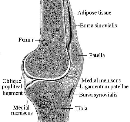
Figure 1: Schematic latero-frontal view of the left knee joint. Although designed to perform mainly flexion/extension (strictly in the sagittal plane) with some restricted medial/lateral rotation in the semi-flexed position, it is clear that the knee joint really has at least 6 degrees-of-freedom, including 3 micro–translations. The injury actually occurs when some of these microscopic translations become macroscopic, which normally happens only after an external jolt.

Knee joint injuries range from mild ligament or meniscus tearing to severe traumatic dislocations (see [Seroyer et al 2008] and references therein) that fall among the most severe form of ligament injury to the lower extremity, associated with a high rate of complications including amputation.

Knee joint injuries are also frequent in sports, especially in ball games. For example, in a recently case–reported complex knee injury in a rugby league player [Shillington et al 2008], resulting in combined rupture of the patellar tendon, anterior cruciate and medial collateral ligaments, with a medial meniscal tear, the video–analysis suggests two points during the tackle when there was the potential for injury: the first occurred when the player was in single leg stance whilst running and received impact to his upper body from three defenders; the second occurred when the player landed on the knee and sustained a valgus and hyper-flexion force under the weight of two defenders. The goal of treatment in this condition is restoration of both the extensor mechanism and knee stability.

Also, the increased number of women participating in sports like soccer has been paralleled by a greater knee injury rate in women compared to men. In particular, menstrual cycle phase has been correlated with risk of noncontact anterior cruciate ligament injury in women (see, e.g. [Chaudhari et al 2007]). Among these injuries, those occurring to the anterior cruciate ligament are commonly observed during sidestep cutting maneuvers [Sanna and O’Connor 2008]. In addition, general fatigue appears to correlate with injuries to the passive knee–joint structures during a soccer game. It has been observed that a higher injury rate and more severe injuries occur towards the end of a soccer game or practice [Hawkins et al 2001, Ostenberg and Roos 2000], suggesting a fatigue effect on the neuromuscular system. Besides, women soccer players who sustain knee injuries have a high risk of going on to develop osteoarthritis at a young age [Lohmander et al 2004].

Besides, the knee is the body part most commonly injured as a consequence of collisions, falls, and overuse occurring from childhood sports. The number of sports–related injuries is increasing because of active participation of children in competitive sports [Siow et al 2008]. Children differ from adults in many areas, such as increased rate and ability of healing, higher strength of ligaments compared with growth plates, and continued growth. Growth around the knee can be affected if the growth plates are involved in injuries [Siow et al 2008].

Literature on knee mechanics has been reviewed in [Komistek et al 2005], evaluating various techniques that had been used to determine in ‘vivo loads’ in the human knee joint. Two main techniques that had been used were 3-axial accelerometer-based telemetry – an experimental approach, and mathematical modelling – a theoretical approach. Accelerometric analyzes had previously been used to determine the ‘in vivo’ loading of the human hip and more recently evaluated in the determination of in vivo knee loads. Mathematical modelling approaches can be categorized in two ways: (i) those that use optimization techniques to solve an indeterminate system, and (ii) those that utilize a reduction method that minimizes the number of unknowns, keeping the system solvable as the number of equations of motion are equal to the number of unknown quantities (for more technical details, see [Komistek et al 2005] and references therein).

The use of a force–controlled dynamic knee simulator to quantify the mechanical performance of total knee replacement designs during functional activity was pioneered by [DesJardins et al 2000], in which dynamic total knee replacement (TKR) study utilized a 6-degree-of-freedom force–controlled knee simulator to quantify the effect of TKR design alone on TKR mechanics during a simulated walking cycle. Simultaneous prediction of implant kinematics and contact mechanics has been demonstrated using explicit finite element (FE) models of the Instron/Stanmore Knee Joint Simulator, Instron, Canton, MA [Godest et al 2002, Halloran et al 2005a, Halloran et al 2005b] In these models, kinematic verification was performed by comparing experimental and model-predicted motion for a single implant. Both models were found to produce similar kinematic simulation results. Estimated contact pressure distributions were also closely correlated, as long as significant edge–loading conditions were not present. Recently, an adaptive FE method for pre–clinical wear testing of TKR components was developed in [Knight et al 2007], capable of simulating wear of a polyethylene tibial insert and to compare predicted kinematics, weight loss due to wear, and wear depth contours to results from a force–controlled experimental knee simulator. The displacement–controlled inputs, by accurately matching the experimental tibio-femoral motion, provided an evaluation of the simple wear theory. The force–controlled inputs provided an evaluation of the overall numerical method by simultaneously predicting both kinematics and wear. Proposed international standards for TKR wear simulation have been drafted (see [ISO Standard 14243-2, 2000]), yet their methods continue to be debated [Laz et al, 2005]. The ‘gold standard’ to which all TKR wear testing methodologies should be compared is measured in vivo TKR performance in patients. The study of [DesJardins et al 2007] compared patient TKR kinematics from fluoroscopic analysis and simulator TKR kinematics from force–controlled wear testing to quantify similarities in clinical ranges of motion and contact bearing kinematics and to evaluate the proposed ISO force–controlled Stanmore wear testing methodology.

For human movement purposes, we can say that the safe knee motions (flexion/extension with some medial/lateral rotation in the flexed position) are governed by standard Euler’s rotational dynamics coupled to Newton’s micro-translational dynamics. On the other hand, the unsafe knee events, in this paper we will show that the main cause of knee injuries are the knee SE(3)–jolts, the sharp and sudden, “delta”– (forces + torques) combined. These knee SE(3)–jolts do not belong to the standard Newton–Euler dynamics. The only way to monitor them would be to measure “in vivo” the rate of the combined (forces + torques)– rise in the knee joint (see Figure 1).

This paper proposes a new hypothesis for generic musculo-skeletal injury, called:

Coupled–loading–rate hypothesis:
The main cause of knee injury is Euclidean jolt, or $SE(3)-$jolt, an impulsive loading that hits the knee joint in several coupled degrees-of-freedom (DOF) simultaneously. The same hypothesis applies to any other major human joint: all acute musculo-skeletal injuries are caused by some form of Euclidean jolt.

In the realm of musculo-skeletal injury, a Euclidean jolt represents a 6-degree-of-freedom ‘jerk’ (rate-of-change of acceleration) times most-of-the-body mass. In other words, a Euclidean jolt is a time derivative of the Euclidean force (three-dimensional force + three-dimensional torque). In the case of a knee, it happens when all the body mass is on one leg with a semi-flexed knee – and then, caused by some external shock, the knee ‘jerks’; this often happens in running, skiing, sports games (e.g., soccer, rugby) and various crashes/impacts. The reason why this happens in this particular scenario is the following: in a semi-flexed position, the knee joint has all 6 DOF; if a sudden jerk with the full body mass hits the knee in this position, it will happen in all 6 DOF simultaneously, tearing apparat the soft tissue. If the resulting jolt is of high intensity then even the hard tissue will be damaged.

To demonstrate this formally, based on the previously defined covariant force law, we formulate the coupled Newton–Euler dynamics of the knee motions and derive from it the corresponding coupled $SE(3)-$jolt dynamics. The effect of $SE(3)-$jolt can be seen in two forms of discontinuous knee injury: (i) mild rotational disclinations and (ii) severe translational dislocations. Both the knee disclinations and dislocations, as caused by the $SE(3)-$jolt, are described using the Cosserat multipolar viscoelastic continuum model.

While we can intuitively visualize the knee SE(3)–jolt, for the purpose of whole human musculo-skeletal dynamics simulation, to avoid deterministic chaos caused by nonlinear coupling, we use the necessary simplified, decoupled approach (neglecting the 3D torque matrix and its coupling to the 3D force vector). In this decoupled framework of reduced complexity, we define:

The cause of knee dislocations is a linear 3D–jolt vector, the time rate-of-change of a 3D–force vector (linear jolt = mass $\times$ linear jerk). The cause of knee disclinations is an angular 3–axial jolt, the time rate-of-change of a 3–axial torque (angular jolt = inertia moment $\times$ angular jerk).

This decoupled framework has been implemented in the Human Biodynamics Engine [Ivancevic 2005], a high-resolution neuro–musculo–skeletal dynamics simulator (with 270 DOFs, the same number of equivalent muscular actuators and two–level neural reflex control), developed by the present author at Defence Science and Technology Organization, Australia. This kinematically validated human motion simulator has been described in a series of papers and books [Ivancevic and Snoswell 2001, Ivancevic and Beagley 2003, Ivancevic 2002, Ivancevic 2004, Ivancevic and Beagley 2005],
[Ivancevic and Ivancevic 2006a, Ivancevic and Ivancevic 2006b, Ivancevic and Ivancevic 2006c],
[Ivancevic and Ivancevic 2007d, Ivancevic and Ivancevic 2007e, Ivancevic 2006, Ivancevic and Ivancevic 2007a, Ivancevic and Ivancevic 2006, Ivancevic and Ivancevic 2007b, Ivancevic and Ivancevic 2008].

2 The $SE(3)-$jolt: the main cause of human joint injury

In the language of modern biodynamics [Ivancevic 2004, Ivancevic and Ivancevic 2006a], the general knee motion is governed by the Euclidean SE(3)–group of 3D motions. Within the knee SE(3)–group we have both SE(3)–kinematics (consisting of the knee SE(3)–velocity and its two time derivatives: SE(3)–acceleration and SE(3)–jerk) and the knee SE(3)–dynamics (consisting of SE(3)–momentum and its two time derivatives: SE(3)–force and SE(3)–jolt), which is the knee kinematics $\times$ the knee mass–inertia distribution.

Informally, the knee SE(3)–jolt is a sharp and sudden change in the SE(3)–force acting on the mass–inertia distribution within the knee joint. That is, a ‘delta’–change in a 3D force–vector coupled to a 3D torque–vector, hitting the knee. In other words, the knee SE(3)–jolt is a sudden, sharp and discontinues shock in all 6 coupled dimensions of the knee joint, within the three Cartesian ($x,y,z$)–translations and the three corresponding Euler angles around the Cartesian axes: roll, pitch and yaw [Ivancevic and Beagley 2003]. If the SE(3)–jolt produces a mild shock to the knee (internal sudden loss of stability), it causes mild, soft–tissue knee injury. If the SE(3)–jolt produces a hard shock (external hit by a massive body) to the knee, it causes severe, hard–tissue knee injury, with the total loss of knee movement.

The knee SE(3)–jolt is rigorously defined in terms of differential geometry
[Ivancevic and Ivancevic 2006c, Ivancevic and Ivancevic 2007e]. Briefly, it is the absolute time–derivative of the covariant force 1–form (or, co-vector field) applied to the knee. With this respect, recall that the fundamental law of biomechanics – the so–called covariant force law [Ivancevic and Ivancevic 2006b, Ivancevic and Ivancevic 2006c, Ivancevic and Ivancevic 2007e], states:

$$\text{Force co-vector field}=\text{Mass distribution}\times\text{Acceleration vector--field},$$

which is formally written (using the Einstein summation convention, with indices labelling the three local Cartesian translations and the corresponding three local Euler angles):

$$F_{{\mu}}=m_{{\mu}{\nu}}a^{{\nu}},\qquad({\mu,\nu}=1,...,6=3\text{ Cartesian}+3\text{ Euler})$$

where $F_{{\mu}}$ denotes the 6 covariant components of the knee SE(3)–force co-vector field, $m_{{\mu}{\nu}}$ represents the 6$\times$6 covariant components of the inertia–metric tensor of the total mass moving in the knee joint, while $a^{{\nu}}$ corresponds to the 6 contravariant components of the knee SE(3)–acceleration vector-field.

Now, the covariant (absolute, Bianchi) time–derivative $\frac{{D}}{dt}(\cdot)$ of the covariant SE(3)–force $F_{{\mu}}$ defines the corresponding knee SE(3)–jolt co-vector field:

$$\frac{{D}}{dt}(F_{{\mu}})=m_{{\mu}{\nu}}\frac{{D}}{dt}(a^{{\nu}})=m_{{\mu}{\nu}}\left(\dot{a}^{{\nu}}+\Gamma_{\mu\lambda}^{{\nu}}a^{{\mu}}a^{{\lambda}}\right),$$ (1)

where ${\frac{{D}}{dt}}{(}a^{{\nu}})$ denotes the 6 contravariant components of the knee SE(3)–jerk vector-field and overdot ($\dot{~{}}$) denotes the time derivative. $\Gamma_{\mu\lambda}^{{\nu}}$ are the Christoffel’s symbols of the Levi–Civita connection for the SE(3)–group, which are zero in case of pure Cartesian translations and nonzero in case of rotations as well as in the full–coupling of translations and rotations.

In the following, we elaborate on the knee SE(3)–jolt concept (using vector and tensor methods) and its biophysical consequences in the form of the knee dislocations and disclinations.

2.1 $SE(3)-$group of local joint motions

Briefly, the $SE(3)-$group of knee motions is defined as a semidirect (noncommutative) product of 3D knee rotations and 3D knee micro–translations,

$$SE(3):=SO(3)\rhd\mathbb{R}^{3}.$$

Its most important subgroups are the following:

In other words, the gauge $SE(3)-$group of knee Euclidean micro-motions contains matrices of the form $\left(\begin{array}[]{cc}\mathbf{R}&\mathbf{p}\\ 0&1\end{array}\right),$ where $\mathbf{p}$ is knee 3D micro-translation vector and $\mathbf{R}$ is knee 3D rotation matrix, given by the product $\mathbf{R}=R_{\varphi}\cdot R_{\psi}\cdot R_{\theta}$ of the three Eulerian knee rotations, $\text{roll}=R_{\varphi},~{}\text{pitch}=R_{\psi},~{}\text{yaw}=R_{\theta}$, performed respectively about the $x-$axis by an angle $\varphi,$ about the $y-$axis by an angle $\psi,$ and about the $z-$axis by an angle $\theta$ (see [Ivancevic 2004, Park and Chung 2005, Ivancevic 2006]),

$$R_{\varphi}=\left[\begin{array}[]{ccc}1&0&0\\ 0&\cos\varphi&-\sin\varphi\\ 0&\sin\varphi&\cos\varphi\end{array}\right],~{}~{}R_{\psi}=\left[\begin{array}[]{ccc}\cos\psi&0&\sin\psi\\ 0&1&0\\ -\sin\psi&0&\cos\psi\end{array}\right],~{}~{}R_{\theta}=\left[\begin{array}[]{ccc}\cos\theta&-\sin\theta&0\\ \sin\theta&\cos\theta&0\\ 0&0&1\end{array}\right].$$

Therefore, natural knee $SE(3)-$dynamics is given by the coupling of Newtonian (translational) and Eulerian (rotational) equations of the knee motion.

2.2 Local joint $SE(3)-$dynamics

To support our locally–coupled loading–rate hypothesis, we formulate the coupled Newton–Euler dynamics of the knee motions within the $SE(3)-$group. The forced Newton–Euler equations read in vector (boldface) form

Newton $$: ~{}\mathbf{\dot{p}}~{}\mathbf{\equiv M\dot{v}=F+p\times\omega},$$ (2)

Euler $$: ~{}\mathbf{\dot{\pi}}~{}\mathbf{\equiv I\dot{\omega}=T+\pi\times\omega+p\times v},$$

where $\times$ denotes the vector cross product,

$$\mathbf{M}\equiv M_{ij}=diag\{m_{1},m_{2},m_{3}\}\qquad\text{and}\qquad\mathbf{I}\equiv I_{ij}=diag\{I_{1},I_{2},I_{3}\},\qquad(i,j=1,2,3)$$

are the total moving segment’s (diagonal) mass and inertia matrices, defining the total moving segment mass–inertia distribution, with principal inertia moments given in Cartesian coordinates ($x,y,z$) by volume integrals

$$I_{1}=\iiint\rho(z^{2}+y^{2})dxdydz,~{}~{}I_{2}=\iiint\rho(x^{2}+z^{2})dxdydz,~{}~{}I_{3}=\iiint\rho(x^{2}+y^{2})dxdydz,$$

dependent on the knee density $\rho=\rho(x,y,z)$,

$$\mathbf{v}\equiv v^{i}=[v_{1},v_{2},v_{3}]^{t}\qquad\text{and\qquad}\mathbf{\omega}\equiv{\omega}^{i}=[\omega_{1},\omega_{2},\omega_{3}]^{t}$$

(where $[~{}]^{t}$ denotes the vector transpose) are linear and angular knee–velocity vectors (that is, column vectors),

$$\mathbf{F}\equiv F_{i}=[F_{1},F_{2},F_{3}]\qquad\text{and}\qquad\mathbf{T}\equiv T_{i}=[T_{1},T_{2},T_{3}]$$

are gravitational and other external force and torque co-vectors (that is, row vectors) acting on the knee,

$$\mathbf{p} \equiv p_{i}\equiv\mathbf{Mv}=[p_{1},p_{2},p_{3}]=[m_{1}v_{1},m_{2}v_{2},m_{2}v_{2}]\qquad\text{and}$$

$$\mathbf{\pi} \equiv \pi_{i}\equiv\mathbf{I\omega}=[\pi_{1},\pi_{2},\pi_{3}]=[I_{1}\omega_{1},I_{2}\omega_{2},I_{3}\omega_{3}]$$

are linear and angular knee–momentum co-vectors.

In tensor form, the forced Newton–Euler equations (2) read

$$\dot{p}_{i} \equiv M_{ij}\dot{v}^{j}=F_{i}+\varepsilon_{ik}^{j}p_{j}{\omega}^{k},\qquad(i,j,k=1,2,3)$$

$$\dot{\pi}_{i} \equiv I_{ij}\dot{\omega}^{j}=T_{i}+\varepsilon_{ik}^{j}\pi_{j}\omega^{k}+\varepsilon_{ik}^{j}p_{j}v^{k},$$

where the permutation symbol $\varepsilon_{ik}^{j}$ is defined as

$$\varepsilon_{ik}^{j}=\begin{cases}+1&\text{if }(i,j,k)\text{ is }(1,2,3),(3,1,2)\text{ or }(2,3,1),\\ -1&\text{if }(i,j,k)\text{ is }(3,2,1),(1,3,2)\text{ or }(2,1,3),\\ 0&\text{otherwise: }i=j\text{ or }j=k\text{ or }k=i.\end{cases}$$

In scalar form, the forced Newton–Euler equations (2) expand as

Newton $$: \left\{\begin{array}[]{c}\dot{p}_{{}_{1}}={F_{1}}-{m_{3}}{v_{3}}{\omega_{2}}+{m_{2}}{v_{2}}{\omega_{3}}\\ \dot{p}_{{}_{2}}={F_{2}}+{m_{3}}{v_{3}}{\omega_{1}}-{m_{1}}{v_{1}}{\omega_{3}}\\ \dot{p}_{{}_{3}}={F_{3}}-{m_{2}}{v_{2}}{\omega_{1}}+{m_{1}}{v_{1}}{\omega_{2}}\end{array}\right.,$$ (6)

Euler $$: \left\{\begin{array}[]{c}\dot{\pi}_{{}_{1}}={T_{1}}+({m_{2}}-{m_{3}}){v_{2}}{v_{3}}+({I_{2}}-{I_{3}}){\omega_{2}}{\omega_{3}}\\ \dot{\pi}_{{}_{2}}={T_{2}}+({m_{3}}-{m_{1}}){v_{1}}{v_{3}}+({I_{3}}-{I_{1}}){\omega_{1}}{\omega_{3}}\\ \dot{\pi}_{{}_{3}}={T_{3}}+({m_{1}}-{m_{2}}){v_{1}}{v_{2}}+({I_{1}}-{I_{2}}){\omega_{1}}{\omega_{2}}\end{array}\right.,$$ (10)

showing the moving segment’s mass and inertia couplings.

Equations (2)–(6) can be derived from the translational + rotational kinetic energy of the moving segment

$$E_{k}={\frac{1}{2}}\mathbf{v}^{t}\mathbf{Mv}+{\frac{1}{2}}\mathbf{\omega}^{t}\mathbf{I\omega},$$ (11)

or, in tensor form

$$E={\frac{1}{2}}M_{ij}{v}^{i}{v}^{j}+{\frac{1}{2}}I_{ij}{\omega}^{i}{\omega}^{j}.$$

For this we use the Kirchhoff–Lagrangian equations (see, e.g., [Lamb 1932, Leonard 1997], or the original work of Kirchhoff in German)

$$\frac{d}{{dt}}\partial_{\mathbf{v}}E_{k} = \partial_{\mathbf{v}}E_{k}\times\mathbf{\omega}+\mathbf{F},$$ (12)

$${\frac{d}{{dt}}}\partial_{\mathbf{\omega}}E_{k} = \partial_{\mathbf{\omega}}E_{k}\times\mathbf{\omega}+\partial_{\mathbf{v}}E_{k}\times\mathbf{v}+\mathbf{T},$$

where $\partial_{\mathbf{v}}E_{k}=\frac{\partial E_{k}}{\partial\mathbf{v}},~{}\partial_{\mathbf{\omega}}E_{k}=\frac{\partial E_{k}}{\partial\mathbf{\omega}}$; in tensor form these equations read

$$\frac{d}{dt}\partial_{v^{i}}E = \varepsilon_{ik}^{j}\left(\partial_{v^{j}}E\right)\omega^{k}+F_{i},$$

$$\frac{d}{dt}\partial_{{\omega}^{i}}E = \varepsilon_{ik}^{j}\left(\partial_{{\omega}^{j}}E\right){\omega}^{k}+\varepsilon_{ik}^{j}\left(\partial_{v^{j}}E\right)v^{k}+T_{i}.$$

Using (11)–(12), linear and angular knee–momentum co-vectors are defined as

$$\mathbf{p}=\partial_{\mathbf{v}}E_{k}{,\qquad\mathbf{\pi}=\partial_{\mathbf{\omega}}E_{k},}$$

or, in tensor form

$$p_{i}=\partial_{v^{i}}E{,\qquad}\pi_{i}=\partial_{{\omega}^{i}}E,$$

with their corresponding time derivatives, in vector form

$$~{}\mathbf{\dot{p}}=\frac{d}{dt}\mathbf{p=}\frac{d}{dt}\partial_{\mathbf{v}}E{,\qquad\mathbf{\dot{\pi}}=}\frac{d}{dt}\mathbf{\pi=}\frac{d}{dt}\partial_{\mathbf{\omega}}E,$$

or, in tensor form

$$~{}\dot{p}_{i}=\frac{d}{dt}p_{i}=\frac{d}{dt}\partial_{v^{i}}E{,\qquad\dot{\pi}_{i}=}\frac{d}{dt}\pi_{i}=\frac{d}{dt}\partial_{{\omega}^{i}}E,$$

or, in scalar form

$$\mathbf{\dot{p}}=[\dot{p}_{1},\dot{p}_{2},\dot{p}_{3}]=[m_{1}\dot{v}_{1},m_{2}\dot{v}_{2},m_{3}\dot{v}_{3}],\qquad{\mathbf{\dot{\pi}}}=[\dot{\pi}_{1},\dot{\pi}_{2},\dot{\pi}_{3}]=[I_{1}\dot{\omega}_{1},I_{2}\dot{\omega}_{2},I_{3}\dot{\omega}_{3}].$$

While healthy knee $SE(3)-$dynamics is given by the coupled Newton–Euler micro–dynamics, the knee injury is actually caused by the sharp and discontinuous change in this natural $SE(3)$ micro-dynamics, in the form of the $SE(3)-$jolt, causing discontinuous knee deformations, both translational dislocations and rotational disclinations.

2.3 Joint injury dynamics: the $SE(3)-$jolt

The $SE(3)-$jolt, the actual cause of the knee injury (in the form of the plastic deformations), is defined as a coupled Newton+Euler jolt; in (co)vector form the $SE(3)-$jolt reads

$$SE(3)-\text{jolt}:\left\{\begin{array}[]{l}\text{Newton~{}jolt}:\mathbf{\dot{F}=\ddot{p}-\dot{p}\times\omega-p\times\dot{\omega}}~{},\\ \text{Euler~{}jolt}:\mathbf{\dot{T}=\ddot{\pi}}~{}\mathbf{-\dot{\pi}\times\omega-\pi\times\dot{\omega}-\dot{p}\times v-p\times\dot{v}},\end{array}\right.$$

where the linear and angular jolt co-vectors are

$$\mathbf{\dot{F}\equiv M\ddot{v}}=[\dot{F}_{{1}},\dot{F}_{{2}},\dot{F}_{{3}}],\qquad\mathbf{\dot{T}\equiv I\ddot{\omega}}=[\dot{T}_{{1}},\dot{T}_{{2}},\dot{T}_{{3}}],$$

where

$$\mathbf{\ddot{v}}=[\ddot{v}_{{1}},\ddot{v}_{{2}},\ddot{v}_{{3}}]^{t},\qquad\mathbf{\ddot{\omega}}=[\ddot{\omega}_{{1}},\ddot{\omega}_{{2}},\ddot{\omega}_{{3}}]^{t},$$

are linear and angular jerk vectors.

In tensor form, the $SE(3)-$jolt reads

$$~{}\dot{F}_{i} = \ddot{p}_{i}-\varepsilon_{ik}^{j}\dot{p}_{j}{\omega}^{k}-\varepsilon_{ik}^{j}p_{j}{\dot{\omega}}^{k},\qquad(i,j,k=1,2,3)$$

$$~{}\dot{T}_{{i}} = \ddot{\pi}_{i}~{}-\varepsilon_{ik}^{j}\dot{\pi}_{j}\omega^{k}-\varepsilon_{ik}^{j}\pi_{j}{\dot{\omega}}^{k}-\varepsilon_{ik}^{j}\dot{p}_{j}v^{k}-\varepsilon_{ik}^{j}p_{j}\dot{v}^{k},$$

in which the linear and angular jolt covectors are defined as

$$\mathbf{\dot{F}} \equiv \dot{F}_{i}=\mathbf{M\ddot{v}}\,\equiv\mathbf{\,}M_{ij}\ddot{v}^{j}=[\dot{F}_{1},\dot{F}_{2},\dot{F}_{3}],$$

$$\mathbf{\dot{T}} \equiv \dot{T}_{{i}}=\mathbf{I\ddot{\omega}\equiv\,}I_{ij}\ddot{\omega}^{j}=[\dot{T}_{{1}},\dot{T}_{{2}},\dot{T}_{{3}}],$$

where  $\mathbf{\ddot{v}}=\ddot{v}^{{i}},$ and $\mathbf{\ddot{\omega}}=\ddot{\omega}^{{i}}$ are linear and angular jerk vectors.

In scalar form, the $SE(3)-$jolt expands as

Newton jolt $$: \left\{\begin{array}[]{l}\dot{F}_{{1}}=\ddot{p}_{1}-m_{{2}}\omega_{{3}}\dot{v}_{{2}}+m_{{3}}\left({\omega}_{{2}}\dot{v}_{{3}}+v_{{3}}\dot{\omega}_{{2}}\right)-m_{{2}}v_{{2}}{\dot{\omega}}_{{3}},\\ \dot{F}_{{2}}=\ddot{p}_{2}+m_{{1}}\omega_{{3}}\dot{v}_{{1}}-m_{{3}}\omega_{{1}}\dot{v}_{{3}}-m_{{3}}v_{{3}}\dot{\omega}_{{1}}+m_{{1}}v_{{1}}\dot{\omega}_{{3}},\\ \dot{F}_{{3}}=\ddot{p}_{3}-m_{{1}}\omega_{{2}}\dot{v}_{{1}}+m_{{2}}\omega_{{1}}\dot{v}_{{2}}-v_{{2}}\dot{\omega}_{{1}}-m_{{1}}v_{{1}}\dot{\omega}_{{2}},\end{array}\right.$$

Euler jolt $$: \left\{\begin{array}[]{l}\dot{T}_{{1}}=\ddot{\pi}_{1}-(m_{{2}}-m_{{3}})\left(v_{{3}}\dot{v}_{{2}}+v_{{2}}\dot{v}_{{3}}\right)-(I_{{2}}-I_{{3}})\left(\omega_{{3}}\dot{\omega}_{{2}}+{\omega}_{{2}}{\dot{\omega}}_{{3}}\right),\\ \dot{T}_{{2}}=\ddot{\pi}_{2}+(m_{{1}}-m_{{3}})\left(v_{{3}}\dot{v}_{{1}}+v_{{1}}\dot{v}_{{3}}\right)+(I_{{1}}-I_{{3}})\left({\omega}_{{3}}{\dot{\omega}}_{{1}}+{\omega}_{{1}}{\dot{\omega}}_{{3}}\right),\\ \dot{T}_{{3}}=\ddot{\pi}_{3}-(m_{{1}}-m_{{2}})\left(v_{{2}}\dot{v}_{{1}}+v_{{1}}\dot{v}_{{2}}\right)-(I_{{1}}-I_{{2}})\left({\omega}_{{2}}{\dot{\omega}}_{{1}}+{\omega}_{{1}}{\dot{\omega}}_{{2}}\right).\end{array}\right.$$

We remark here that the linear and angular momenta ($\mathbf{p,\pi}$), forces ($\mathbf{F,T}$) and jolts ($\mathbf{\dot{F},\dot{T}}$) are co-vectors (row vectors), while the linear and angular velocities ($\mathbf{v,\omega}$), accelerations ($\mathbf{\dot{v},\dot{\omega}}$) and jerks ($\mathbf{\ddot{v},\ddot{\omega}}$) are vectors (column vectors). This bio-physically means that the ‘jerk’ vector should not be confused with the ‘jolt’ co-vector. For example, the ‘jerk’ means shaking the head’s own mass–inertia matrices (mainly in the atlanto–occipital and atlanto–axial joints), while the ‘jolt’means actually hitting the head with some external mass–inertia matrices included in the ‘hitting’ SE(3)–jolt, or hitting some external static/massive body with the head (e.g., the ground – gravitational effect, or the wall – inertial effect). Consequently, the mass-less ‘jerk’ vector represents a (translational+rotational) non-collision effect that can cause only soft knee injuries, while the inertial ‘jolt’ co-vector represents a (translational+rotational) collision effect that can cause hard knee injuries.

2.4 Joint disclinations and dislocations caused by the $SE(3)-$jolt

For mild knee injury (caused by internal loss of stability), the best injury predictor is considered to be the product of localized knee strain and strain rate, which is the standard isotropic viscoelastic continuum concept (see, e.g. [Halloran et al 2005a]). To improve this standard concept, in this subsection, we consider the knee joint as a 3D anisotropic multipolar Cosserat viscoelastic continuum [Cosserat and Cosserat 1898, Cosserat and Cosserat 1909, Eringen 2002], exhibiting coupled–stress–strain elastic properties. This non-standard continuum model is suitable for analyzing plastic (irreversible) deformations and fracture mechanics [Bilby and Eshelby 1968] in multi-layered materials with microstructure (in which slips and bending of layers introduces additional degrees of freedom, non-existent in the standard continuum models; see [Mindlin 1965, Lakes 1985] for physical characteristics and [Yang and Lakes 1981, Yang and Lakes 1982],
[Park and Lakes 1986] for biomechanical applications).

The $SE(3)-$jolt $(\mathbf{\dot{F},\dot{T}})$ causes two types of localized knee discontinuous deformations:

1. The Newton jolt $\mathbf{\dot{F}}$ can cause severe micro-translational dislocations, or discontinuities in the Cosserat translations;

2. The Euler jolt $\mathbf{\dot{T}}$ can cause mild micro-rotational disclinations, or discontinuities in the Cosserat rotations.

For general treatment on dislocations and disclinations related to asymmetric discontinuous deformations in multipolar materials, see, e.g., [Jian and Xiao-ling 1995, Yang et al 2001].

To precisely define the knee dislocations and disclinations, caused by the $SE(3)-$jolt $(\mathbf{\dot{F},\dot{T}})$, we first define the coordinate co-frame, i.e., the set of basis 1–forms $\{dx^{i}\}$, given in local coordinates $x^{i}=(x^{1},x^{2},x^{3})=(x,y,z)$, attached to the moving segment’s center-of-mass. Then, in the coordinate co-frame $\{dx^{i}\}$ we introduce the following set of the knee plastic–deformation–related $SE(3)-$based differential $p-$forms (see [Ivancevic and Ivancevic 2006c, Ivancevic and Ivancevic 2007e]):
    the dislocation current 1–form, $\mathbf{J}=J_{i}\,dx^{i};$
    the dislocation density 2–form, $\mathbf{\alpha}=\frac{1}{2}\alpha_{ij}\,dx^{i}\wedge dx^{j};$
    the disclination current 2–form, $\mathbf{S}=\frac{1}{2}S_{ij}\,dx^{i}\wedge dx^{j};$  and
    the disclination density 3–form, $\mathbf{Q}=\frac{1}{3!}Q_{ijk}\,dx^{i}\wedge dx^{j}\wedge dx^{k}$,

where $\wedge$ denotes the exterior wedge–product. According to Edelen [Edelen 1980, Kadic and Edelen 1983], these four $SE(3)-$based differential forms satisfy the following set of continuity equations:

$$\mathbf{\dot{\alpha}}=\mathbf{-dJ-S,}$$ (15)

$$\mathbf{\dot{Q}}=\mathbf{-dS,}$$ (16)

$$\mathbf{d\alpha}=\mathbf{Q,}$$ (17)

$$\mathbf{dQ}=\mathbf{0,}\qquad$$ (18)

where $\mathbf{d}$ denotes the exterior derivative.

In components, the simplest, fourth equation (18), representing the Bianchi identity, can be rewritten as

$$\mathbf{dQ}=\partial_{l}Q_{[ijk]}\,dx^{l}\wedge dx^{i}\wedge dx^{j}\wedge dx^{k}=0,$$

where $\partial_{i}\equiv\partial/\partial x^{i}$, while $\theta_{[ij...]}$ denotes the skew-symmetric part of $\theta_{ij...}$.

Similarly, the third equation (17) in components reads

$$\frac{1}{3!}Q_{ijk}\,dx^{i}\wedge dx^{j}\wedge dx^{k} = \partial_{k}\alpha_{[ij]}\,dx^{k}\wedge dx^{i}\wedge dx^{j},\text{\qquad or}$$

$$Q_{ijk} = -6\partial_{k}\alpha_{[ij]}.$$

The second equation (16) in components reads

$$\frac{1}{3!}\dot{Q}_{ijk}\,dx^{i}\wedge dx^{j}\wedge dx^{k} = -\partial_{k}S_{[ij]}\,dx^{k}\wedge dx^{i}\wedge dx^{j},\text{\qquad or}$$

$$\dot{Q}_{ijk} = 6\partial_{k}S_{[ij]}.$$

Finally, the first equation (15) in components reads

$$\frac{1}{2}\dot{\alpha}_{ij}\,dx^{i}\wedge dx^{j} = (\partial_{j}J_{i}-\frac{1}{2}S_{ij})\,dx^{i}\wedge dx^{j},\text{\qquad or}$$

$$\dot{\alpha}_{ij}\, = 2\partial_{j}J_{i}-S_{ij}\,.$$

In words, we have:

• The 2–form equation (15) defines the time derivative $\mathbf{\dot{\alpha}=}\frac{1}{2}\dot{\alpha}_{ij}\,dx^{i}\wedge dx^{j}$ of the dislocation density $\mathbf{\alpha}$ as the (negative) sum of the disclination current $\mathbf{S}$ and the curl of the dislocation current $\mathbf{J}$. This time derivative is caused by the translational part of the SE(3) jolt.

• The 3–form equation (16) states that the time derivative $\mathbf{\dot{Q}=}\frac{1}{3!}\dot{Q}_{ijk}\,dx^{i}\wedge dx^{j}\wedge dx^{k}$ of the disclination density $\mathbf{Q}$ is the (negative) divergence of the disclination current $\mathbf{S}$. This time derivative is caused by the rotational part of the SE(3) jolt.

• The 3–form equation (17) defines the disclination density $\mathbf{Q}$ as the divergence of the dislocation density $\mathbf{\alpha}$, that is, $\mathbf{Q}$ is the exact 3–form.

• The Bianchi identity (18) follows from equation (17) by Poincaré lemma [Ivancevic and Ivancevic 2006c, Ivancevic and Ivancevic 2007e] and states that the disclination density $\mathbf{Q}$ is conserved quantity, that is, $\mathbf{Q}$ is the closed 3–form. Also, every 4–form in 3D space is zero.

From these equations, we can conclude that the knee dislocations and disclinations are mutually coupled by the underlaying $SE(3)-$group, which means that we cannot separately analyze translational and rotational knee injuries. This result supports the validity of the combined loading hypothesis.

3 Conclusion

Based on the previously developed covariant force law [Ivancevic and Ivancevic 2006a, Ivancevic and Ivancevic 2007e], its recent application to traumatic brain injury [Ivancevic 2008], and using as an example a human knee joint, in this paper we have formulated a new coupled loading–rate hypothesis for the generic musculo-skeletal injury. This new injury hypothesis states that generic cause of human joint injuries is an external $SE(3)-$jolt, an impulsive loading hitting a joint in several degrees-of-freedom, both rotational and translational, combined and simultaneously. To demonstrate this, we have developed the vector Newton–Euler mechanics on the Euclidean $SE(3)-$group of the knee micro-motions. In this way, we have precisely defined the concept of the $SE(3)-$jolt, which is a cause of two kinds of rapid joint discontinuous deformations: (i) mild rotational disclinations, and (ii) severe translational dislocations. Based on the presented model, we argue that we cannot separately analyze localized joint rotations from translations, as they are in reality coupled. To prevent human musculo-skeletal injuries we need to develop the musculo-skeletal SE(3)–jolt awareness, e.g. never overload a flexed knee, avoid any kind of collisions.

References

- [Ivancevic 2008] Ivancevic, V.G., New mechanics of traumatic brain injury. Cogn. Neurodyn. Online first, Springer, (2008)
- [Seroyer et al 2008] Seroyer, S.T., Musahl, V., Harner, C.D. Management of the acute knee dislocation: The Pittsburgh experience. Injury (Elsevier), 39(7), 710–718, (2008)
- [Shillington et al 2008] Shillington, M., Logan, M., Myers, P. A complex knee injury in a rugby league player Combined rupture of the patellar tendon, anterior cruciate and medial collateral ligaments, with a medial meniscal tear. Injury Extra (Elsevier), in press, available online PubMed, (2008)
- [Chaudhari et al 2007] Chaudhari, A.M.W., Lindenfeld, T.N., Andriacchi, T.P., Hewett, T.E., Riccobene, J., Myer, G.D., Noyes, F.R. Knee and Hip Loading Patterns at Different Phases in the Menstrual Cycle: Implications for the Gender Difference in Anterior Cruciate Ligament Injury Rates. Am. J. Sp. Med. 35, 793-800, (2007)
- [Sanna and O’Connor 2008] Sanna, G., O’Connor, K.M. Fatigue-related changes in stance leg mechanics during sidestep cutting maneuvers. Clin. Biomech. (in press), available online PubMed, (2008)
- [Hawkins et al 2001] Hawkins, R.D., Hulse, M.A., Wilkinson, C., Hodson, A., Gibson, M. The association football medical research programme: an audit of injuries in professional football. Br. J. Sp. Med. 35(1), 43 47, (2001)
- [Ostenberg and Roos 2000] Ostenberg, A., Roos, H. Injury risk factors in female European football. A prospective study of 123 players during one season. Sc. J. Med. Sci. Sp. 10(5) 279 285, (2000)
- [Lohmander et al 2004] Lohmander, L.S., Ostenberg, A., Englund, M. High prevalence of knee osteoarthritis, pain and functional limitations in female soccer players twelve years after anterior cruciate ligament injury. Arthr. Rheum. 50, 3145-3152, (2004)
- [Siow et al 2008] Siow, H.M., Cameron, D.B., Ganley, T.J. Acute Knee Injuries in Skeletally Immature Athletes. Phys. Med. Rehab. 19(2), 319–345, (2008)
- [Komistek et al 2005] Komistek, R.D., Kane, T.R., Mahfouz, M., Ochoa, J.A., Dennis, D.A. Knee mechanics: a review of past and present techniques to determine in vivo loads. J. Biomech. 38(2), 215–228, (2005)
- [Brand et al 1994] Brand, R.A., Pedersen, D.R., Davy, D.T., Kotzar, G.M., Heiple, K.G., Goldberg, V.M. Comparison of hip force calculations and measurements in the same patient. J. Arthroplasty 9(1), 45 51, (1994)
- [DesJardins et al 2000] DesJardins, J.D., Walker, P.S., Haider, H., Perry, J. The use of a force-controlled dynamic knee simulator to quantify the mechanical performance of total knee replacement designs during functional activity. J. Biomech. 33, 1231–1242, (2000)
- [Godest et al 2002] Godest, A.C., Beaugonin, M., Haug, E., Taylor, M., Gregson, P.J. Simulation of a knee joint replacement during a gait cycle using explicit finite element analysis, J. Biomech. 35(2), 267 -275, (2002)
- [Halloran et al 2005a] Halloran, J.P., Easley, S.K., Petrella, A.J., Rullkoetter, P. Comparison of deformable and elastic foundation finite element simulations for predicting knee replacement mechanics. J. Biomech. Eng. 127, 813 818, (2005)
- [Halloran et al 2005b] Halloran, J.P., Petrella, A.J., Rullkoetter, P. Explicit finite element modeling of TKR mechanics. J. Biomech. 38, 323 -331, (2005)
- [Knight et al 2007] Knight, L.A., Pal, S., Coleman, J.C., Bronson, F., Haider, H., Levine, D.L., Taylor, M., Rullkoetter, P.J. Comparison of long-term numerical and experimental total knee replacement wear during simulated gait loading. J. Biomech. 40, 1550–1558, (2007)
- [ISO Standard 14243-2, 2000] Wear of total knee-joint prostheses, Part 2: Methods of measurement. International Standards Organization, (2000)
- [Laz et al, 2005] Laz, P.J., Pal, S., Halloran, J.P., Petrella, A.J., Rullkoetter, P.J. Probabilistic finite element prediction of knee wear simulator mechanics. J. Biomech. 39, 2303-2310, (2005)
- [DesJardins et al 2007] DesJardins, J.D., Banks, S.A., Benson, L.C., Pace, T., LaBerge, M. A direct comparison of patient and force-controlled simulator total knee replacement kinematics. J. Biomech. 40, 3458-3466, (2007)
- [Whiting and Zernicke 1998] Whiting, W.C., Zernicke, R.F. Biomechanics of Musculoskeletal Injury. Human Kinetics, Champaign, IL, (1998).
- [Ivancevic and Snoswell 2001] Ivancevic, V., Snoswell, M. Fuzzy-Stochastic Functor Machine for General Humanoid-Robot Dynamics. IEEE Trans. Sys. Man Cyber. B, 31(3), 319-330, (2001).
- [Ivancevic 2002] Ivancevic, V. Generalized Hamiltonian Biodynamics and Topology Invariants of Humanoid Robots. Int. J. Math. & Math. Sci. 31(9), 555-565, (2002).
- [Ivancevic 2004] Ivancevic, V. Symplectic Rotational Geometry in Human Biomechanics. SIAM Rev. 46(3), 455–474, (2004).
- [Ivancevic 2005] Ivancevic, V. Human Biodynamics Engine – Full Spine Simulator. Australian Defence Excellence in Science & Technology Award 2005 for Physiological Modelling, Adelaide, (2005).
- [Ivancevic and Beagley 2005] Ivancevic, V., Beagley, N. Brain-like functor control machine for general humanoid biodynamics. Int. J. Math. & Math. Sci. 11, 1759-1779, (2005).
- [Ivancevic 2006] Ivancevic, V., Lie-Lagrangian model for realistic human bio-dynamics. Int. J. Hum. Rob. 3(2), 205-218, (2006).