The Cost of Probabilistic Agreement in Oblivious Robot Networks

Abstract

In this paper we address the complexity issues of two agreement problems in oblivious robot networks namely gathering and scattering. These abstractions are fundamental coordination problems in cooperative mobile robotics. Moreover, their oblivious characteristics makes them appealing for self-stabilization since they are self-stabilizing with no extra-cost. Given a set of robots with arbitrary initial location and no initial agreement on a global coordinate system, gathering requires that all robots reach the exact same but not predetermined location while scattering aims at scatter robots such that no two robots share the same location. Both deterministic gathering and scattering have been proved impossible under arbitrary schedulers therefore probabilistic solutions have been recently proposed.

The contribution of this paper is twofold. First, we propose a detailed complexity analysis of the existent probabilistic gathering algorithms in both fault-free and fault-prone environments. Moreover, using Markov chains tools and additional assumptions on the environment we prove that the gathering convergence time can be reduced from $O(n^{2})$ (the best known tight bound) to $O(nln(n))$. Additionally, we prove that in crash-prone environments gathering is achieved in $O(nln(n)+2f)$. Second, using the same technique we prove that the best known scattering strategy converges in fault-free systems is $O(n)$ (which is one to optimal) while in crash-prone environments it needs $O(n-f)$. Finally, we conclude the paper with a discussion related to different strategies to gather oblivious robots.

1 Introduction

Many applications of mobile robotics envision groups of mobile robots self-organizing and cooperating toward the resolution of common objectives. In many cases, the group of robots is aimed at being deployed in adverse environments, such as space, deep sea, or after some natural (or unnatural) disaster. It results that the group must self-organize in the absence of any prior infrastructure (e.g., no global positioning), and ensure coordination in spite of faulty robots and unanticipated changes in the environment.

Suzuki and Yamashita [8] proposed a formal model to analyze and prove the correctness of agreement problems in robot networks. In this model, robots are represented as points that evolve on a plane. At any given time, a robot can be either idle or active. In the latter case, the robot observes the locations of the other robots, computes a target position, and moves toward it. The time when a robot becomes active is governed by an activation daemon (scheduler). Between two activations robots forget the past computations. Interestingly, any algorithm proved correct in this model is also self-stabilizing.

The gathering problem, also known as the Rendez-Vous problem, is a fundamental coordination problem in oblivious mobile robotics. In short, given a set of robots with arbitrary initial location and no initial agreement on a global coordinate system, gathering requires that all robots, following their algorithm, reach the exact same location—one not agreed upon initially—within a finite number of steps, and remain there. The dual of the gathering problem is the scattering problem. Started in a arbitrary configuration scattering requires that eventually no two robots share the same position. Both scattering and gathering are agreement problems and similar to the consensus problem in conventional distributed systems, they have simple definitions but the existence of a solution greatly depends on the synchrony of the systems as well as the nature of the faults that may possibly occur. The task becomes even harder since robots are anonymous since the impossibility results proved in classical distributed computing also hold in robot networks. Therefore, specific problems like flocking, gathering or scattering are impossible without additional assumption. Interestingly, most of the work done so far in order to convey the above impossibility results focuses on the additional assumptions the system needs, less attention being shown to the use of randomization. Surprisingly, no formal framework was proposed in order to analyze the correctness and the complexity of probabilistic algorithms designed for robots networks. In a companion paper, [1], we investigated some of the fundamental limits of deterministic and probabilistic gathering face to a broad synchrony and fault assumptions. Probabilistic scattering, was analyzed for the first time in [2]. None of the previously mentioned works focus on a framework in order to compute the complexity of proposed solutions.

In this paper we advocate that Markov chains are a simple and efficient tool to analyze and compare probabilistic strategies in both fault-free and fault-prone oblivious robot networks. Note that in robot networks computations depend only on the current view of the robots without the use of the past. This behavior makes Markov chains an appealing tool for analyzing their correctness and complexity since by definition a Markov chain models systems where the next configuration depends strictly on the current configuration. The only difficulty while using Markov chains is to associate to each probabilistic strategy the appropriate Markov chain. In the current work we focus on the analysis of existing probabilistic strategies for scattering and gathering and advocate that our analysis can be easily applied to a broad class of probabilistic strategies (e.g. leader election, flocking, constrained scattering, pattern formation).

Contribution

Our contribution is twofold. First, we show that the time complexity of probabilistic gathering in fault-free environments can be improved from $O(n^{2})$ to $O(nln(n))$ when the algorithms exploit additional information related to the environment (eg. multiplicity knowledge). Additionally, in crash-prone environments we prove that the convergence time of gathering is $O(nln(n)+2f)$. Second, we show that the tight bound for scattering is $O(n)$ (which is one to optimal) in fault-free systems while in crash-prone environments scattering converges is $O(n-f)$ rounds where $f$ is the maximal bound on the number of faults. Intuitively gathering and scattering should have the same complexity however our analysis shows that scattering is much easier to obtain than gathering, $O(n)$ versus $O(nln(n))$. Reducing the gap in complexity between gathering and scattering seems to be an interesting research direction as it will be discussed in Section 7.

Structure of the paper

The paper is structured as follows. Section 2 describes the robots network and system model. Section 3 formally defines the gathering and scattering problems. We propose the complexity analysis of existent probabilistic scattering and gathering in Sections 5 and 6 in fault-free and fault-prone environments. In Section 7 we analyze an alternative strategy to gather oblivious robots. Section 8 concludes the paper and discusses some open problems.

2 Model

In the following we propose the model of our system. Most of the definitions are borrowed from [8, 6].

Robot networks.

We consider a network of a finite set of robots arbitrarily deployed in a geographical area. The robots are devices with sensing, computational and motion capabilities. They can observe (sense) the positions of other robots in the plane and based on these observations they perform some local computations. Furthermore, based on the local computations robots may move to other locations in the plane.

In the case robots are able to sense the whole set of robots they are referred as robots with unlimited visibility; otherwise robots have limited visibility. In this paper, we consider that robots have unlimited visibility.

In the case robots are able to distinguish if there are more than one robot at a given position they are referred as robots with multiplicity knowledge.

System model.

A network of robots that exhibit a discrete behavior can be modeled with an I/O automaton [3]. A network of robots that exhibit a continuous behavior can be modeled with a hybrid I/O automaton [4]. This framework allows the modeling of systems that exhibit both a discrete and continuous behavior and in particular the modeling of robots networks.

The actions performed by the automaton modeling a robot are as follows:

• Observation (input type action).
  An observation returns a snapshot of the positions of all the robots in the visibility range. In our case, this observation returns a snapshot of the positions of all the robots;

• Local computation (internal action).
  The aim of a local computation is the computation of a destination point;

• Motion (output type action).
  This action commands the motion of robots towards the destination location computed in the local computation action.

The local state of a robot at time $t$ is the state of its input/output variables and the state of its local variables and registers. A network of robots is modeled by the parallel composition of the individual automata that model one per one the robots in the network. A configuration of the system at time $t$ is the union of the local states of the robots in the system at time $t$. An execution $e=(c_{0},\ldots,c_{t},\ldots)$ of the system is an infinite sequence of configurations, where $c_{0}$ is the initial configuration of the system, and every transition $c_{i}\rightarrow c_{i+1}$ is associated to the execution of a subset of the previously defined actions.

Schedulers.

A scheduler decides at each configuration the set of robots allowed to perform their actions. A scheduler is fair if, in an infinite execution, a robot is activated infinitely often. In this paper we consider the fair version of the following schedulers:

• centralized: at each configuration a single robot is allowed to perform its actions;

• probabilistic: at each configuration a set of robots chosen uniformly is activated;

• $k$-bounded: between two consecutive activations of a robot, another robot can be activated at most $k$ times;

• arbitrary: at each configuration an arbitrary subset of robots is activated.

Faults.

In this paper, we address the following failures:

• crash failures: In this class, we further distinguish two subclasses: (1) robots physically disappear from the network, and (2) robots stop all their activities, but remain physically present in the network;

• Byzantine failures: In this case, robots may have an arbitrary behavior.

Computational models.

The literature proposes two computational models: ATOM and CORDA. The ATOM model was introduced by Suzuki and Yamashita [8]. In this model each robot performs, once activated by the scheduler, a computation cycle composed of the following three actions: observation, computation and motion. The particularity of the ATOM model versus the CORDA model is that in ATOM a computation cycle is atomic while in CORDA the atomicity concerns only the actions. In order words CORDA models and asynchronous networks while ATOM a synchronous one.

In this paper, we consider the ATOM model. Moreover, we consider that robots are oblivious (i.e., stateless). That is, robots do not conserve any information between two computational cycles. We also assume that all the robots in the system have unlimited visibility.

3 Gathering and Scattering

A network of robots is in a legitimate configuration with respect to the gathering requirement if all robots in the system share the same position in the plane. Let denote by ${\mathcal{P}}_{\mathit{Gathering}}$ this predicate.

An algorithm solves the gathering problem in an oblivious system if the following two properties are verified:

• Convergence Any execution of the system starting in an arbitrary configuration reaches in a finite number of steps a configuration that satisfies $\mathcal{P}_{Gathering}$.

• Closure Any execution starting in a legitimate configuration with respect to the $\mathcal{P}_{\mathit{Gathering}}$ predicate contains only legitimate configurations.

Gathering is difficult to achieve in most of the environments. Therefore, weaker forms of gathering were studied so far. An interesting version of this problem requires robots to converge toward a single location rather than reach that location in a finite time. The convergence is however considerably easier to deal with. For instance, with unlimited visibility, convergence can be achieved trivially by having robots moving toward the barycenter of the network [8].

Scattering, introduced first in [7], aims at arranging a set of robots such that eventually no two robots share the same position. Let denote by ${\mathcal{P}}_{Scattering}$ this predicate. Formally, scattering is defined by the following two properties :

• Convergence Any execution of the system starting in an arbitrary configuration reaches in a finite number of steps a configuration that satisfies $\mathcal{P}_{Scattering}$.

• Closure Any execution starting in a legitimate configuration with respect to the predicate ${\mathcal{P}}_{Scattering}$ contains only legitimate configurations.

In the sequel we address the convergence time of gathering and scattering in both fault-free and fault-prone environments. As stated in the model we consider both crash-prone and byzantine-prone systems. Let $(n,f)$ denote a system with $n$ correct robots but $f$ and the considered faults are crashes and byzantine behavior. As mentioned in Section 2 in a $(n,f)$ crash-prone system there are two types of crashes: (1) the crashed robots completely disappear from the system, and (2) the crashed robots are still physically present in the system, however they stop the execution of any action. In [1], we proved that if the faulty robots disappear from the system, then the problem trivially reduces to the study of its fault-free version with $n\!-\!f$ correct robots. In contrast, in systems where faulty robots remain physically present in the network after crashing, the problem is far from being trivial. A similar argument can be provided for the case of byzantine behavior. Obviously, gathering or scattering all the robots in the system including the faulty ones is impossible since faulty robots may possibly have crashed at different locations or collude as shown in [1]. Therefore, we study the feasibility of weaker versions of gathering and scattering, referred to as weak gathering respectively weak scattering. The $(n,f)$-weak problem requires that, in a terminal configuration, only the correct robots must verify the specification.

4 Analysis framework

In this section we introduce some notations and definitions that will be further used in order to analyze the convergence time of the probabilistic gathering and scattering. A detailed description of the notions defined below can be found in [5].

Random variables

We denote $X_{n}$ a random variable. For instance, in our case it might be the number of groups of size $x$ after $n$ steps of the algorithm. We will study a discrete-time stochastic process, that is : a sequence $\{X_{n}\}_{n\geq 0}$ of random variables.

In the sequel we will use the following notations:

• $\mathbb{P}[X_{n}=x]$ the probability of the event $\{X_{n}=x\}$.

• $\mathbb{E}[X_{n}]$ the expectation of $X_{n}$ .

• The probability distribution of a random variable $X:k\mapsto\mathbb{P}[X=k]$ for all $k$

• Conditional probability will be written $\mathbb{P}[A\mid B]$, and will be read ”the probability of A, given B”.

Markov chains

Markov chains are particular classes of stochastic processes. These stochastic processes have the following fundamental property : the probabilistic dependence on the past is only related to the previous state.

Definition 1

Let $\left(X_{n}\right)_{n\in\mathbb{N}}$ be a discrete time stochastic process with countable state space $E$. If for all integers $n\geq 0$ and all states $i_{0},i_{1},\ldots,i_{n-1},i,j$:

$$\mathbb{P}[X_{n+1}=j\mid X_{n}=i,X_{n-1}=i_{n-1},\ldots,X_{0}=i_{0}]=\mathbb{P}[X_{n+1}=j\mid X_{n}=i]$$

Whenever both sides of the above equality are well defined, this stochastic process is called Markov chain. A Markov chain is homogeneous (HMC) if the right side is independent of $n$.

In the following we propose an example of Markov chain.

Toy example 1

Consider a robot performing a random walk in a two-dimensional space. The robot at position $(i,j)$ chooses with equal probability as destination point a neighbor of $(i,j)$ in the space $\mathbb{Z}\times\mathbb{Z}$. Let $X_{n}$ be the robot position after $n$ steps:

• $\mathbb{P}[X_{n+1}=(i,j)\mid X_{n}=(i-1,j)]=1/4$

• $\mathbb{P}[X_{n+1}=(i,j)\mid X_{n}=(i,j-1)]=1/4$

• $\mathbb{P}[X_{n+1}=(i,j)\mid X_{n}=(i+1,j)]=1/4$

• $\mathbb{P}[X_{n+1}=(i,j)\mid X_{n}=(i,j+1)]=1/4$

Note 1

Note that Toy Example 1 is a Markov Chain since every position of the robot is only dependent on the previous one.

In this paper we advocate that Markov chains are a simple verification tool, perfectly adapted to the analysis of distributed strategies in oblivious robot networks since in these networks the next move of a robot depends only on its current position.

5 Probabilistic Gathering

In this section we analyze the complexity of probabilistic gathering in fault-free and fault-prone environments. The algorithms analyzed in this section were proposed in [1].

5.1 Gathering in fault-free environments

In this section we prove that additional information on the environment drastically improves the time convergence of gathering. Using multiplicity knowledge, for example, we obtain a tight bound of $O(nln(n))$ which improves the best known bound of $O(n^{2})$. In [1] we proposed a probabilistic algorithm that solves the fault-free gathering in ATOM, under a special class of schedulers, known as $k$-bounded schedulers. A robot, when chosen by the scheduler, selects randomly one of its neighbors and moves towards its position with probability $\frac{1}{\delta}$ where $\delta$ is the size of the robot’s view. In the considered model the robots have unlimited visibility and the value of $\delta$ is $n$. We proved that this strategy probabilistically solves $2$-gathering in the ATOM model under an arbitrary scheduler and converges in $2$ steps in expectation. We also proved that it solves the $n$-gathering problem ($n\geq 3$), under a fair $k$-bounded scheduler without multiplicity knowledge and converges under fair bounded schedulers in $n^{2}$ rounds in expectation.

In the following we show that the $O(n^{2})$ complexity bound can be reduced to $O(nln(n))$ when robots use the multiplicity. The algorithm that meets this bound was initially proposed in [1] in order to cope with robots crash. The algorithm, shown as Algorithm 5.1, works as follows. When a robot is chosen by the scheduler moves to a group with maximal multiplicity. When several groups have the same maximal multiplicity, then a robot member of such group tosses a coin to decide if it moves or holds the current position. Interestingly, the multiplicity knowledge (used so far in order to break the symmetry of the system) can also be used in order to fasten gathering.

Functions:
                          $\mathit{observe\_neighbors}::$ returns the set of robots within the
                          vision range of robot $p$ (the set of $p$’s neighbors);
                          $\mathit{maximal\_multiplicity}::$ returns the set of robots with the
                          maximal multiplicity;
                          Actions:
                              ${\mathcal{A}}_{1}::\ true\longrightarrow$
                                    $\mathcal{N}_{p}=\mathit{observe\_neighbors}()$;
                                    if $p\in\mathit{maximal\_multiplicity}(\mathcal{N}_{p})\wedge\left|\mathit{maximal\_multiplicity}\left(\mathcal{N}_{p}\right)\right|>1$ then
                                            with probability $\frac{1}{\left|\mathit{maximal\_multiplicity}\left(\mathcal{N}_{p}\right)\right|}$do
                                                     select a robot $q\in\mathit{maximal\_multiplicity}(\mathcal{N}_{p})$;
                                                     move towards $q$;
                                    else
                                            select a robot $q\in\mathit{maximal\_multiplicity}(\mathcal{N}_{p})$;
                                            move towards $q$;

Algorithm 5.1 Probabilistic gathering for robot $p$ with multiplicity knowledge.

Lemma 1

In a fault-free environment the convergence time of Algorithm 5.1 is $\alpha_{n}ln(\alpha_{n})+1$, with $\alpha_{n}=[\frac{n}{2}]+1$.

• In order to study the convergence time of Algorithm 5.1 we introduce the following stochastic process : $\forall\ t,~{}\ X_{t}=k$ means that at round $t$ the group with the maximal multiplicity has $k$ robots. Note that when $k$ equals $1$ all robots are scattered such that no two robots share the same position. Figure 1 proposes the probability transition of the random variable $X_{t}$.

 
 

Figure 1: The stochastic process $X_{t}$ associated to Algorithm 5.1

As soon as a group of $[\frac{n}{2}]+1$ robots is formed, the convergence needs only one additional round. That is, this group will be the unique group of maximal cardinality. Therefore it will be an attractor for all the other robots and within one additional round the convergence is achieved. In the following we compute the time needed to the stochastic process $(X_{t})_{(t\in\mathbb{N}^{*})}$ to reach $[\frac{n}{2}]+1$. We define the expectation of the time needed for the stochastic process $X_{t}$ defined above to reach state $k$, starting from state $l$. Formally,

$$T_{l}^{k}=\mathbb{E}\left[min\{t\ \text{such that}\ X_{t}=k\ \text{knowing}\ X_{0}=l\}\right]$$

According to Figure 1 we obtain the following induction formula:

$$T_{l}^{k}=1+\frac{l}{n}T_{l}^{k}+\frac{n-l}{n}T_{l+1}^{k}$$

which leads to $(T_{l}^{k}-T_{l+1}^{k})=\frac{n}{n-l}$. Therefore, if we note $\alpha_{n}=[\frac{n}{2}]+1$

$$T_{1}^{\alpha_{n}}=\displaystyle\sum_{k=1}^{\alpha_{n}-1}\frac{\alpha_{n}}{\alpha_{n}-k}=\displaystyle\alpha_{n}\sum_{k=1}^{\alpha_{n}-1}\frac{1}{k}\leq\alpha_{n}ln(\alpha_{n})$$

 

5.2 Gathering in Fault-prone environments

In this section we study the complexity of gathering in both crash and byzantine prone systems. We prove that crash tolerant gathering can be achieved in $O(nln(n)+2f)$ while byzantine tolerant gathering is exponential and needs additional assumptions (e.g. probabilistic scheduler).

5.2.1 Crash-tolerant gathering

In [1] we proved the impossibility of deterministic and probabilistic weak gathering (gathering of correct robots) under centralized bounded and fair schedulers and without additional assumptions. An immediate consequence of this result is the necessity of additional assumptions (e.g., multiplicity knowledge), even for probabilistic solutions under bounded schedulers. In the following we study the complexity of Algorithm 5.1 in fault-prone environments.

In order to compute the convergence of Algorithm 5.1 we consider the worst scenario. Recall that in a fault-free environment as soon a group of $[\frac{n}{2}]+1$ robots is built, only one additional round is required to reach convergence. Our scenario goes as follows. Assume that as soon as the group of maximal cardinality has $[\frac{n}{2}]+1$ robots, a crash occurs so that the stochastic chain goes one step backward. We recall that only $f$ crashes may happen. The following lemma computes the convergence time of Algorithm 5.1 according to the above described scenario.

Lemma 2

In a crash prone environment the convergence time of Algorithm 5.1 is $O\left(\alpha_{n}ln(\alpha_{n})+2f\right)$ with $\alpha_{n}=[\frac{n}{2}]+1$.

• We define the following stochastic process to compute the convergence time of the algorithm in a crash prone environment. $\forall\ t,~{}~{}\ Y_{t}=k$ means that, at round $t$, the group with the maximal cardinality has $k$ robots. The system transitions are as follows:

  • $\mathbb{P}[Y_{t}=k\mid Y_{t-1}=k]=\frac{k}{n}$

  • $\mathbb{P}[Y_{t}=k\mid Y_{t-1}=k-1]=\frac{n-k}{n}$

  • Moreover, each time a crash occurs, the stochastic process goes backward.

According to Lemma 1 the group of maximal cardinality of $\frac{n}{2}$ robots is formed within $\alpha_{n}ln(\alpha_{n})$ rounds. In the following we focus the time needed to the chain associated with Algorithm 5.1 to move from state $\alpha_{n}-1$ to $\alpha_{n}$. The probability transition of this event is $\mathbb{P}[Y_{t}=\alpha_{n}\mid Y_{t-1}=\alpha_{n}-1]=\frac{n-\alpha_{n}}{n}$. The mathematical expectation of the time needed to perform this transition is : $\frac{n}{n-\alpha_{n}}\approx 2$. Therefore, the convergence time of Algorithm 5.1 is $\alpha_{n}ln(\alpha_{n})+2f$.  

Note 2

Note that the above results hold even if the crashed robots are still physically present in the system but stop the execution of any action.

5.2.2 Byzantine-tolerant gathering

In this section we address the complexity of byzantine-tolerant probabilistic gathering. In the following $(n,f)$ denotes a system where at most $f$ robots can have byzantine behavior.

In [1] we conjectured that Algorithm 5.1 also solves $(n,f)$-weak byzantine-tolerant gathering problem when $n\geq 3$ under bounded schedulers and multiplicity detection. The counter-example shown in Figure 2 advocates that the boundedness of the scheduler should depend on the ration between correct and byzantine robots otherwise the algorithm does not converge. That is, assume an execution starting in a configuration with two groups of two robots each and assume the right group has a byzantine robot (the robot in red on the picture). The scheduler chooses one robot in the left group and moves it in the right group. Then it chooses the byzantine robot which (even if multiplicity is used) moves in the left group. Then the scheduler chooses any correct robot in the right group and moves it in the left group. Then the byzantine is chosen and moves to the right group. This configuration is symmetrical to the initial configuration.

                             

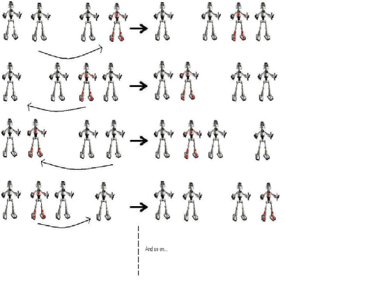
Figure 2: Counter Example: Algorithm 5.1 does not solve the problem under an arbitrary bounded scheduler

However byzantine-tolerant gathering is possible under special conditions. The next lemma proves that byzantine-tolerant gathering is possible when both the algorithm and the scheduler are probabilistic. Here we use the power of random choice. That is, there is a positive probability that the byzantine robot is not chosen in a finite number of steps.

Lemma 3

In systems with Byzantine faults, Algorithm 5.1 probabilistically solves the $(n,f)$-weak byzantine-tolerant gathering, $n\geq 3$, problem under a probabilistic scheduler and multiplicity detection.

• The proof is based on the fact that as soon as there exists a group of $\frac{N}{2}+1$ correct robots gathered, an additional round is needed to achieve convergence That is, every time a correct robot is selected by the scheduler, it joins this group. Therefore, beyond this point, the convergence time only depends on the scheduler.

  In the following we study the probability to create a group verifying the above stated property. We define $\mathcal{L}$ : There exists a group of $\frac{N}{2}+1$ correct robots gathered.

  $$\mathbb{P}\left[\ \text{reach}\ \mathcal{L}\ \text{in}\ \frac{N}{2}+1\ \text{steps}\right]>\displaystyle\left(\frac{1}{N}\right)^{(\frac{N}{2}+1)}=\varepsilon$$

  So

  $$\mathbb{P}\left[\neg(\text{reach}\ \mathcal{L}\ \text{in}\ (\frac{N}{2}+1)\ \text{steps})\right]\leq(1-\varepsilon)$$

  Therefore :

  $$\forall k,\ \mathbb{P}\left[\neg(\text{reach}\ \mathcal{L}\ \text{in}\ k(\frac{N}{2}+1)\ \text{steps})\right]\leq(1-\varepsilon)^{k}$$

  $$\displaystyle\lim_{k\rightarrow\infty}\mathbb{P}\left[\neg(\text{reach}\ \mathcal{L}\ \text{in}\ k(\frac{N}{2}+1)\ \text{steps})\right]=0$$

   

Note that in our scenario the convergence time is exponential. In order to simplify the calculations we consider: $\left(\frac{1}{N}\right)^{N}$ instead of $\left(\frac{1}{N}\right)^{(\frac{N}{2}+1)}$.

So, $\left[1-\left(\frac{1}{N}\right)^{N}\right]^{t}\leq\alpha$. This leads to:

$$tln\left(1-\left(\frac{1}{N}\right)^{N}\right)\leq ln\alpha$$

Overall, $t$ verifies:

$$t\geq\frac{ln\alpha}{ln\left(1-\left(\frac{1}{N}\right)^{N}\right)}\sim\ln\left(\frac{1}{\alpha}\right)N^{N}$$

Remark 1

In order to prove the convergence we considered one of the worst possible scenario. Therefore, we did not prove that the convergence time of the algorithm is exponential. In order to do so, we would have to exhibit a set of non-null measure of executions which converges in an exponential time.

6 Probabilistic scattering

In this section we address another agreement problem : the scattering. The unique existing probabilistic solution for scattering was proposed in [2] (see Algorithm 6.1). Analyzing the complexity of Algorithm 6.1 in both fault-free and fault-prone environments we prove that scattering is much easier to achieve than gathering. The next section addresses Algorithm 6.1 convergence in fault-free environments then we prove the correctness and compute the complexity of the same algorithm in fault-prone systems.

6.1 Scattering in Fault-free environments

Petit et al. [2] proved that deterministic scattering is impossible in ATOM model without additional assumptions and proposed a probabilistic solution based on the use of Voronoi diagrams defined below.

Definition 2

Let ${\mathcal{P}}=\{p_{1},p_{2},\ldots,p_{n}\}$ be a set of points in the Cartesian 2-dimensional plane. The Voronoi diagram of ${\mathcal{P}}$ is a subdivision of the plane into $n$ cells, one for each point in ${\mathcal{P}}$. The cells have the property that a point $q$ belongs to the Voronoi cell of point $p_{i}$ iff for any other point $p_{j}\in{\mathcal{P}}$, $dist(q,p_{i})<dist(q,p_{j})$ where $dist(p,q)$ is the Euclidean distance between $p$ and $q$. In particular, the strict inequality means that points located on the boundary of the Voronoi diagram do not belong to any Voronoi cell.

The algorithm proposed in [2] (see Algorithm 6.1) is as follows. Each robot uses a function $Random()$ that returns a value probabilistically chosen in the set $\{0,1\}$ : $0$ with probability $\frac{3}{4}$ and $1$ with probability $\frac{1}{4}$. When a robot $r_{i}$ becomes active at time $t$, it first computes the Voronoi Diagram of $P_{r_{i}}(t)$, i.e., the set of points occupied by the robots. Then, $r_{i}$ moves toward a point inside its Voronoi $Cell_{i}$ if $Random()$ returns $0$.

Compute the Voronoi Diagram;
$Cell_{i}:=$ the Voronoi cell where $r_{i}$ is located; .
$Current\_Pos:=$ position where $r_{i}$ is located;

If $Random()=0$
then Move toward an arbitrary position in $Cell_{i}$, different from $Current\_Pos$;

Algorithm 6.1 Probabilistic Scattering executed by robot $r_{i}$.

In the following we study the convergence time of Algorithm 6.1.

Lemma 4

The convergence time of Algorithm 6.1 is $O(n)$.

• In order to study the convergence time of this algorithm we introduce the following stochastic process : $X_{t}=k$ means that at time $t$ there are $k$ different Voronoi cells.

  Let us consider the worst scenario : If $X_{t}=k$, we assume that there are $k-1$ robots at $k-1$ different positions and $n-k+1$ robots at the exact same position. Therefore, our stochastic process has the probability transitions given in Figure 3.

   
   

  Figure 3: The stochastic process $X_{t}$ associated to Algorithm 6.1

For all $k\in\{1,\ldots,n\}$ let $T_{l}^{k}$ be the time for the stochastic process to enter in $k$, starting from $l$. Based on the above notation and the chain proposed in Figure 3 we obtain the following induction formula :

$$\forall k\in\mathbb{N},~{}T_{l}^{k+1}=1+(1-\alpha^{n-(k-1)})T_{l}^{k}+\alpha^{n-(k-1)}T_{l}^{k+1}$$

where $\alpha=\frac{1}{4}$. This leads to $T_{l}^{k+1}-T_{l}^{k}=\frac{1}{1-\alpha^{n-(k-1)}}$. If we sum from $0$ to $n-1$ we get :

$$T_{1}^{n}=\sum_{k=0}^{n-1}\frac{1}{1-\alpha^{n-(k-1)}}=\sum_{j=0}^{n-1}\frac{1}{1-\alpha^{j}}$$

This sequence does not converge since $\displaystyle\lim_{j\rightarrow\infty}\frac{1}{1-\alpha^{j}}\neq 0$. Furthermore $\displaystyle\frac{1}{1-\alpha^{j}}\mathop{\sim}_{j\rightarrow\infty}1+\alpha^{j}$. Thus the partial sums are equivalent :

$$T_{1}^{n}\mathop{\sim}_{n\rightarrow\infty}\sum_{j=0}^{n-1}1+\alpha^{j}$$

Since $\sum_{j=0}^{n-1}(1+\alpha^{j})=n+\sum_{j=0}^{n-1}\alpha^{j}$ we finally obtain : $T_{1}^{n}\displaystyle\mathop{\sim}_{n\rightarrow\infty}n+\frac{4}{3}$  

6.2 Scattering in fault-prone environments

In this section we analyze the correctness and the complexity of Algorithm 6.1 in crash-prone environments. Note that Algorithm 6.1 is not byzantine resilient. In the sequel we denote by $(n,f)$ systems with $n$ robots where $f$ is the maximal number of crashed robots. Note that scattering is impossible in systems where nodes may crash since faulty nodes may share the same position. Therefore, we consider in the following a weaker version of scattering, weak scattering that requires the verification of the scattering specification only from correct nodes.

Lemma 5

Algorithm 6.1 eventually verifies the $(n,f)$ weak scattering specification under a weakly fair scheduler.

• In the case when the $f$ faulty nodes disappear from the network the convergence proof is similar to the convergence of the system when the number of robots is $n-f$ (see [2]).

  Let consider systems where the faulty robots are still present in the system. Let ${\mathcal{M}}$ be the set of correct robots whom position is occupied by another robot (faulty or correct). In the following we show that starting in a illegitimate configuration (${\mathcal{M}}\neq\emptyset$) the system converges with positive probability in a finite number of steps to a configuration where ${\mathcal{M}}=\emptyset$. Let call the latter configuration legitimate.

  Consider an execution, $e$, starting in a illegitimate configuration, $c$ (${\mathcal{M}}\neq\emptyset$ in $c$). Assume the scheduler does not choose robots in ${\mathcal{M}}$. Then, it may choose either faulty robots or correct robots not in ${\mathcal{M}}$ (i.e. these robots do not share their position with any other robot). In both cases, the size of ${\mathcal{M}}$ does not increase. Since the scheduler is weakly fair it will eventually choose at least one robot in ${\mathcal{M}}$. Let $m\geq 1$ be the number of robots chosen by the scheduler. Either all the $m$ robots choose randomly to stay or leave the current position or some of them crash. In both cases the size of ${\mathcal{M}}$ decreases by at least one robot. With positive probability, $p\geq\frac{3}{4}(\frac{1}{4})^{m-1}$ this robot will change its position to a new position in its Voronoi cell and hence the size of ${\mathcal{M}}$ decreases by at least one. Recursively repeating the same argument, in a finite number of steps, the size of ${\mathcal{M}}$ drops to 0 with positive probability.  

Lemma 6

The convergence time of Algorithm 6.1 in systems with $n$ correct robots but $f$ is $O(n)$.

• The idea of the proof is similar to the one presented in Section 6. Consider a random variable $Y_{t}$ with values in $\{0$..$n\}$. $Y_{t}=k$ iff there is a set ${\cal M}$ of $k$ non faulty robots in which each robot shares its position with another robot. Our goal is to compute the time before $Y_{k}$ reaches $0$. Note that the presence of faulty robots can only accelerate the process (see the proof of Lemma 5). That is, if a robot of the set ${\cal M}$ crashes, our random variable is decreased by $1$. Hence the convergence time is upper bounded by $n-f+\frac{4}{3}$.  

7 How to gather oblivious robots?

In Section 5 we analyzed a possible strategy to gather robots that converges in $O(nln(n))$ in fault-free environments and in $O(nln(n)+2f)$ in crash-proned systems. In Section 6 we computed the complexity of a scattering strategy that is one of optimal (i.e. $O(n)$ in fault-free environments and $O(n-f)$ in fault-prone environments). Interestingly, even if both strategies solve an agreement problem there is an important complexity gap between the existing implementations of gathering and scattering. An interesting open question is how to reduce this gap. That is, how to implement gathering in order to match the $O(n)$ lower bound?

In this section we discuss a promising alternative to obtain gathering. The gathering algorithm proposed in [2] is built on top of the probabilistic scattering algorithm shown in Figure 6.1 and works as follows: if there exist at least two positions with strict multiplicity then apply the scattering procedure otherwise apply any deterministic gathering protocol based on multiplicity knowledge. Note that the above protocol does not verify the gathering specification for the case when the initial configuration does not contain strict multiplicity points. The argument is similar to the one used in order to prove probabilistic gathering impossible under an arbitrary scheduler (see [1]). That is, started in a configuration legitimate for scattering the above algorithm will try to apply the deterministic gathering. Since the gathering algorithm is deterministic several points of strict multiplicity may be created unless the scheduler is restricted to weaker forms (e.g. centralized or bounded). Then, the scattering restarts but the scheduler may “derandomize” the choice of the robots such that all the multiplicity points are simultaneously destroyed. From this point onward one can exhibit an infinite execution in which the system cycles between scattering and gathering without achieving convergence. However, the proposed method becomes interesting in systems where the flip/flop scattering/gathering would be always able to converge to a configuration with an unique strict multiplicity point. Once this point created the system will need a single round to converge. So, far no algorithm responds to these criteria.

8 Conclusions and Discussions

The contribution of this paper is twofold. First, we proposed a detailed complexity analysis of the existent probabilistic agreement algorithms (gathering and scattering) in both fault-free and fault-prone environments. Moreover, using Markov chains tools and multiplicity knowledge we proved that the convergence time of gathering can be reduced from $O(n^{2})$ (the best known tight bound) to $O(nln(n))$. Second, we prove that the best known scattering bound is $O(n)$ (which is one to optimal). Additionally, we proved that in crash-prone environments gathering is achieved in $O(nln(n)+2f)$ rounds while scattering needs $O(n+f)$ rounds. Finally, we proposed a discussion related to the best strategy to design gathering. This work opens several research directions. For example the flip/flop scattering/gathering seems to be a promising direction to reduce the complexity of gathering. Another interesting direction is the complexity of byzantine-tolerant gathering. We conjecture that byzantine-tolerant gathering can be achieved in polynomial time.

References

- [1] Xavier Défago, Maria Gradinariu, Stéphane Messika, and Philippe Raipin Parvédy. Fault-tolerant and self-stabilizing mobile robots gathering. In Shlomi Dolev, editor, DISC, pages 46–60. Springer, 2006.
- [2] Yoann Dieudonné and Franck Petit. Robots and demons (the code of the origins). In FUN, pages 108–119, 2007.
- [3] N. A. Lynch. Distributed Algorithms. Morgan Kaufmann, San Francisco, CA, USA, 1996.
- [4] N. A. Lynch, R. Segala, and F. W. Vaandrager. Hybrid I/O automata. Information and Computation, 185(1):105–157, August 2003.
- [5] J.R. Norris. Markov Chains. Cambridge University Press, 1997.
- [6] G. Prencipe. Corda: Distributed coordination of a set of autonomous mobile robots. In Proc. 4th European Research Seminar on Advances in Distributed Systems (ERSADS’01), pages 185–190, Bertinoro, Italy, May 2001.
- [7] I. Suzuki and M. Yamashita. A theory of distributed anonymous mobile robots formation and agreement problems. Technical report, Wisconsin Univ. Milwakee, Dep. of Electrical Engineering and Computer Science, 1994.
- [8] I. Suzuki and M. Yamashita. Distributed anonymous mobile robots: Formation of geometric patterns. SIAM Journal of Computing, 28(4):1347–1363, 1999.