Splotch: Visualizing Cosmological Simulations

Abstract

We present a light and fast, public available, ray-tracer Splotch software tool which supports the effective visualization of cosmological simulations data. We describe the algorithm it relies on, which is designed in order to deal with point-like data, optimizing the ray-tracing calculation by ordering the particles as a function of their “depth” defined as a function of one of the coordinates or other associated parameter. Realistic three-dimensional impressions are reached through a composition of the final color in each pixel properly calculating emission and absorption of individual volume elements. We describe several scientific as well as public applications realized with Splotch. We emphasize how different datasets and configurations lead to remarkable different results in terms of the images and animations. A few of these results are available online.

1 Introduction

According to the standard theory of the Big Bang, our universe came into existence as a singularity around 13.7 billion years ago. After its initial appearance, it inflated from a very dense, hot and homogeneous state to the expanded, cooled and very structured state of our current universe. During its evolution, planets, stars, galaxies and all the different objects and structures that we observe have formed, as the result of a fine interplay of gravitational forces with a number of different physical processes, like fluid dynamics effects (shock waves, turbulence), magnetic fields, star formation and associated feedback (e.g. supernova explosions). Cosmologists adopt numerical simulations as an effective instrument to describe, investigate and understand the evolution of such a complicated system within the framework of the expanding space-time of the universe. There are various numerical methods – grid or particle based – to perform such simulations. For a recent review on such numerical simulation methods within the cosmological context see Dolag et al. (2008).

The resulting data is huge and complex and requires suitable and effective tools to be inspected and explored. Visualisation represents the most immediate and intuitive way to analyse and explore data and to understand results. Larger and larger data sets require an enormous computational effort to be systematically studied and more and more complex and expensive algorithms to identify patterns and features. Visualisation allows easily to focus on sub-samples and features of interest and to detect correlations and special characteristics of data. This is not a substitute for systematic analysis, but it is a fundamental support to accelerate and simplify the cognitive process.

Visualisation also is an effective instrument to introduce common people, especially young people, to even the most complicated and innovative aspects and concepts of science. The opportunity to use 3D digital visualisation and Virtual Reality facilities, further enhance the impact for the communication and divulgation and push toward a new approach to the cultural and scientific heritage.

The availability of tools to visualise scientific data in a comprehensible, self-describing, rich and appealing way is therefore crucial for researchers and for common people, both for creating knowledge and for disseminating it.

Such tools must be able to deal with a huge data volume, possibly leading to meaningful results in a reasonable time. Furthermore, they must meet the requirements of the particular discipline which produced the data and fit the specific characteristics and peculiarities of the same data. In particular, most of the state-of-the-art cosmological simulations describe the different matter components in the universe (stars, dark matter, gas …) as fluid elements (either point-like or on a regular / irregular grid), which must be properly rendered. For data based on regular grids many visualization packages are available. However, simulations based on a particle-like description of the fluid elements are much more difficult to visualize. There are standard packages like TIPSY or VisIVO for displaying such data, however they are not designed to lead to ray-tracing like images, which might give more realistic impressions of 3D structures ore even artistic like impressions for public outreach.

In this paper we present Splotch, a public ray-tracing software. Splotch is specifically designed to render in a fast and effective way the different families of point-like data, results of a cosmological, but, more generally, astrophysical simulation. Splotch is based on a lightweight and fast algorithm, which will be described in Section 2. Section 3 will present some examples where Splotch was used to produce images for scientific publications and animations presented at various conferences. In Section 4 we describe a 4D Universe project where Splotch was used to produce a public outreach movie which will be shown to the public in the Virtual Reality facility of the brand new Turin Planetarium. We will describe methods used to generate the data used for the Splotch rendering and the technique adopted to create the stereographic version of the movie.

2 Splotch

The underlying visualization algorithm is a derivate of what in general is called volumetric ray casting and uses an approximation of the radiative transfer equation, which – together with the application of perspective – gives the produced images a very realistic appearance, especially when absorption features are present in the cosmological structures which are to be visualized.

2.1 Physical motivation of the algorithm

The rendering algorithm of Splotch is generally designed to handle point-like particle distributions. We especially have Smoothed Particle Hydrodynamic (SPH Lucy, 1977; Gingold and Monaghan, 1977) simulations in mind, where the density of the fluid is described by spreading tracer particles by a kernel, most commonly the $B_{2}$-Spline (Monaghan and Lattanzio, 1985)

$$W(x,h)=\frac{8}{\pi h^{3}}\left\{\begin{array}[]{ll}1-6\left(\frac{x}{h}\right)^{2}+6\left(\frac{x}{h}\right)^{3}&0\leq\frac{x}{h}<0.5\\ 2\left(1-\frac{x}{h}\right)^{3}&0.5\leq\frac{x}{h}<1\\ 0&1\leq\frac{x}{h}\\ \end{array}\right.,$$ (1)

where $h$ is the local smoothing length, which is typically defined in a way that every particle overlaps with $\approx 64$ neighbors. Therefore, the rendering is based on the following assumptions:

• The contribution to the matter density by every particle can be described as a Gaussian distribution of the form $\rho_{p}(\vec{r})=\rho_{0,p}\exp(-r^{2}/\sigma_{p}^{2})$. In practice, it is much more handy to have a compact support of the distribution, and therefore the distribution is set to zero at a given distance of $f\cdot\sigma_{p}$. Following the SPH approach of the original cosmological simulation we choose $f$ in such a way that $f\cdot\sigma_{p}$ is related to the smoothing length $h$, i.e. to fulfill $h\approx f\cdot\sigma_{p}$. Therefore rays passing the particle at a distance larger than $f\cdot\sigma_{p}$ will be practically unaffected by the particle’s density distribution.

• We use three “frequencies” to describe the red, green and blue components of the radiation, respectively. These are treated independently.

• The radiation intensity $\bf{I}$ along a ray through the simulation volume is modeled by the well known radiative transfer equation

  $$\frac{d\bf{I}(x)}{dx}=(\bf{E}_{p}-\bf{A}_{p}\bf{I}(x))\rho_{p}(x),$$ (2)

  which can be found in standard textbooks like Shu (1991). Here, $\bf{E}_{p}$ and $\bf{A}_{p}$ describe the strength of radiation emission and absorption for a given SPH particle for the three rgb-colour components. In general it is recommended to set $\bf{E}_{p}=\bf{}A_{p}$, which typically produces visually appealing images; for special effects, however, independent emission and absorption coefficients can be used. These coefficients can vary between particles, and are typically chosen as a function of a characteristic particle property (e.g. its temperature, density, etc.). The mapping between the scalar property and the three components of $\bf{E}$ and $\bf{A}$ (for red, green and blue) is typically achieved via a colour look-up table or palette, which can be provided to the ray-tracer as an external file to allow a maximum of flexibility.

Assuming that absorption and emission are homogeneously mixed it can be shown that, whenever a ray traverses a particle, its intensity change is given by

$$\bf{I}_{\mbox{after}}=(\bf{I}_{\mbox{before}}-\bf{E}_{p}/\bf{A}_{p})\exp(-\bf{A}_{p}\int_{-\infty}^{\infty}\rho_{p}(x)dx)+\bf{E}_{p}/\bf{A}_{p}$$ (3)

The integral in this equation is given by $\rho_{0,p}\sigma_{p}\exp{(-d_{0}^{2}/\sigma_{p}^{2})}\sqrt{\pi}$, where $d_{0}$ is the minimum distance between the ray and the particle center.

Under the assumption that the SPH particles do not overlap, the intensity reaching the observer could simply be calculated by applying this formula to all particles intersecting with the ray, in the order of decreasing distance to the observer. In reality, of course, the particles do overlap, but since the relative intensity changes due to a single particle can be assumed to be very small, this approach can nevertheless be used in good approximation.

2.2 Implementation of the algorithm

The rendering algorithm now proceeds as follows:

• A camera position $\vec{c}$, a look-at point $\vec{l}$ (e.g. the position of the object of interest) and a sky vector $\vec{s}$ are specified by the user. The latter just defines the up-direction for the scene, and the first two define the viewing direction $\vec{v}$, i.e. $\vec{v}=\vec{l}-\vec{c}$. An example of the simulation geometry is given in figure 5 in section 4.1. Now a linear transformation matrix is determined, which maps $\vec{c}$ to the origin and aligns $\vec{v}$ with the positive $z$-axis. This transformation is applied to all particles. Therefore the ray-tracing can now proceed along the z-axis of the new coordinates, which further simplifies the procedure as well as any further operation like perspective or in field-of-view tests.

• A perspective projection is applied, using a user-defined field-of-view angle $\varphi$.

• The particles are sorted in the order of descending $z$-coordinate of their center. Therefore the ray-tracing (as described in our approximation) can now be achieved by walking the particles and calculating their contribution to the individual pixels of the final image.

• A frame buffer is allocated, which stores an RGB colour triplet for every pixel of the resulting image. This buffer is initialised as black.

• For every particle and every related pixel, equation 3 is used to update the colour value stored in this pixel.

• Once all particles have been processed, the frame buffer contains the final image, which is written to disk in a standard format (e.g. TGA or JPEG).

2.3 Public version of the algorithm

Besides various internal optimisations, Splotch uses OpenMP to generate different regions of the image distributed over several cores on shared memory platforms. The algorithm requires 30 bytes per particle, which allows to render more than 70 million particles on a standard PC with 2 GByte of main memory. Therefore it is applicable to extremely large particle sets, as provided by modern cosmological simulations. The latest version is publically available under GNU General Public License and can be downloaded from http://www.mpa-garching.mpg.de/$\sim$kdolag/Splotch/. The reading routine is optimized to directly read the standard output format of P-GADGET2 (Springel, 2005) and we strongly encourage users to do the adaption to their preferred formats, which can be easily implemented.

2.4 Performance of the algorithm

The CPU time consumption of splotch to render individual frames depends on the frame size, the number of particles to visualize as well as their apparent size, e.g. over how many pixels they get spread. For a typical setup we find $T_{\mathrm{CPU}}\propto n_{\mathrm{pixel}}$ and $T_{\mathrm{CPU}}\propto-0.5\varphi$, e.g. doubling the number of pixels of the final image will double the CPU time, whereas reducing the field-of-view ($\varphi$, typically set to 30 degrees) to halve the value will increase the CPU time by 50%. To measure the performance we re-calculated with the latest version of the code some individual images of movies presented later in this work. As reference system we executed splotch as single task on a AMD Opteton 850 CPU with 2400 MHz. The underlying cosmological simulation for the movie described in section 4 is described by $\approx 11$ million gas particles and $\approx 5$ million star particles, of which a large fraction is usually visible in the individual frames. On our reference system splotch takes $\approx 67$ seconds to render a typical frame (as shown in figure 7) with a resolution of $1400\times 1050$ pixels. The zoomed simulation used for making the movie presented in section 3.2 is represented by a slightly smaller number of gas particles (in this case $\approx 5$ million), but focuses on a smaller region in space revealing more details. To render a typical frame with a resolution of $800\times 800$ pixels splotch takes $\approx 72$ seconds on our reference system. Note that to produce the movies in addition a substantial fraction of time is needed to interpolate the particle files for the individual frames.

3 Application to cosmological simulations

Clusters of galaxies are ideal cosmological probes (See Borgani and Guzzo, 2001, for a review.). They are the largest collapsed objects in the Universe and so are very sensitive to the structure formation process. The evolution of the diffuse cluster baryons (the so-called intra cluster medium, ICM) has a nontrivial interplay with the cosmological environment, as well as with the processes of star formation and evolution of the galaxy population. Modern cosmological, hydro-dynamical simulations are able to model a large variety of physical processes, among them also the energy released by stellar populations and nuclear activity in galaxies and clusters of galaxies, the largest known structures the universe is built of. This energy changes the thermo-dynamical properties of the gas, generates complex patterns in the ICM, so as to regulate the process of gas cooling and star formation. At the same time, the infall of smaller structures within the main cluster regions continuously perturbs the conditions of dynamical equilibrium. This is evident both from the dynamics traced by galaxy motions within and around clusters, and from the presence of prominent features within the ICM (e.g. cold fronts and bow shocks) which represents the signature of merging structures. One of the most common, publically available cosmological simulation codes is P-GADGET2 (Springel, 2005). Highly optimised, it is used to perform some of the largest cosmological simulations available at the moment, including various physical processes at work during the evolution of cosmic structures. The visual representation of the data produced by such simulations can provide substantial help to understand the structure and the dynamics of the matter filling our universe. In the following two sub-sections we show some examples extracted from scientific work presented in astrophysical journals or conferences. In all cases, the vizualisation was based on Splotch.

3.1 Visualisations using flat projection

For visualising cosmological structures it is often useful to adopt a flat projection to obtain the equivalent of a map as obtained from a very distant object. In this case, the raytracing – due to handling of absorption – still can lead to some three-dimensional impression, as becomes apparent in figure 2. Especially in the temperature map (right panel), the interplay between the hot atmosphere (red) and the cold filaments (white), which squeeze like pillars into the atmosphere, is particularly emphasised by the ray-tracing technique used.

Although the ray-tracing algorithm is motivated in the previous section to obtain a realistic, three-dimensional representation, sometimes it can be useful to modify it slightly (in an unphysical manner) to obtain interesting diagnostics of cosmological simulations. Figure 2 shows such an example. To emphasise the presence of small scale substructure, which in the real ray-tracing would be partially (or even fully, if positioned far inside the dense atmosphere) absorbed by the outer parts of the atmosphere, the sorting of the particles is not done according to their spatial position along the z-axis but as a function of relevant scalar quantities associated to each particle (e.g. temperature, metallicity – left panel) or of their density (right panel). Therefore the large amount of small structures (in this case galaxies) and their surrounding becomes clearly visible, as they are passed by the ray only after the rest of the atmosphere is passed. In this way, the 3D impression is obviously lost. Although this kind of maps could be obtained by other adaptive map making algorithms, it is worth mentioning that in Splotch this different behaviour is basically obtained by changing only one parameter which determines the desired sorting technique.

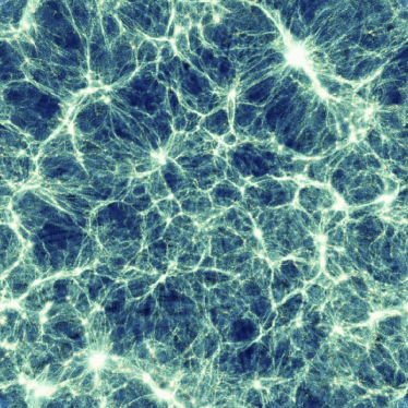
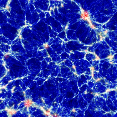
Figure 1: Map of a cosmological simulation box. The light would need nearly $10^{9}$ years to cross the sidelength of the box and the slice thickness correspond to $\approx 50$ million lightyears The largest structure formed in this cosmological simulation (a massive galaxy cluster) can be found in the upper right side of the panel. Left panel is colouring density of the individual particles, right panel is colouring temperature of the individual particles. Taken from Borgani et al. (2004).

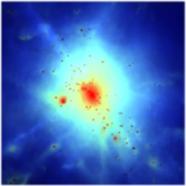
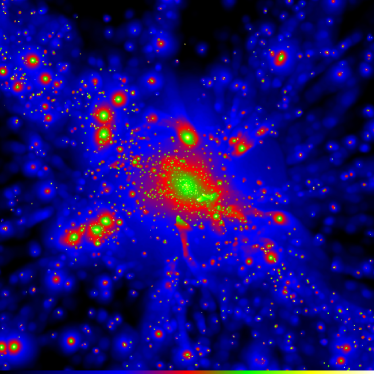
Figure 2: Map of two galaxy clusters using a flat projection, but associating the displayed value in inverse order as “depth”, i.e. ray-tracing from low values to high values. The substructure present in the hot atmosphere of the clusters can be easily recognised. Left panel is taken from Borgani et al. (2004) and the right panel is taken from Borgani et al. (2006).

3.2 Animations of evolving galaxy clusters

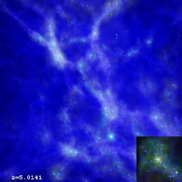
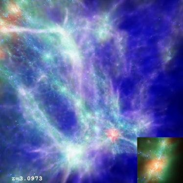
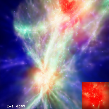
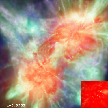
Figure 3: Sequence of ray-tracing the formation and evolution of a galaxy cluster from a high resolution “zoomed” simulation (Borgani et al., 2006). Here, the ray-tracing approach by its absorption feature creates impressive features similar to moving through fog when the camera is passing through small objects on its way around the structure. The upper panels show a region of the universe at an early time. It is rich of filamentary structures, and later, when the universe evolves, almost all these structures are going to collapse to form a single, prominent galaxy cluster. The lower panels show the same region at a later time, where the two main progenitors of the final galaxy cluster are going to merge. The movie can be downloaded from http://www.mpa-garching.mpg.de/galform/data_vis/index.shtml#movie8.

To display the dynamics characterising the formation of galaxy clusters, the realistic, 3D impression obtained when rendering with Splotch results in amazing animations, as shown in Figure 3. This movie is based on processing nearly 250 outputs (each $\approx$1GB in size) of a high resolution, “zoomed” galaxy cluster simulation taken from Borgani et al. (2006), following with the camera a slightly elliptical orbit around the forming object. To obtain the high number of evolving frames, the individual snapshots were interpolated 20 times in a pre-processing step. Therefore a total amount of $\approx 5$TB of temporary particle data were processed to show the evolution of a galaxy cluster from very early times on. The representation starts when the universe has just 5% of its present age, and the first galaxies are forming (around $z\approx 6$). Light would need about 30 millions of years to pass the region of space shown in this animation The images show the intergalactic medium coloured by its temperature. At $z$ around 3.5 the universe has 15% of its current age, and the forming large-scale structure (filaments) can be clearly recognised. The inlay in the lower right shows a zoom into the interior of one of the two prominent proto-clusters. It is the result on a second run of Splotch with different settings and was superimposed to the original frame in a post-processing step. In such structures (clusters of galaxies) several thousands of galaxies can be bound by gravity. At $z$ around 0.8 the universe is half as old as now, and the two prominent proto-clusters begin to merge into one galaxy cluster. Such events are the most energetic phenomena since the universe was born in the Big Bang. In the final phase of this merging event a gigantic shock-wave is initiated, releasing enormous amounts of energy. The shock can be identified as red, out-moving shell. The movie can be downloaded from http://www.mpa-garching.mpg.de/galform/data_vis/index.shtml#movie8, where a number of other movies of evolving galaxy clusters produced with Splotch can be found.

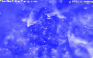
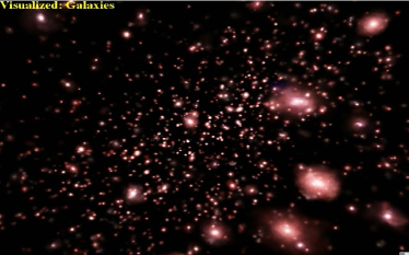
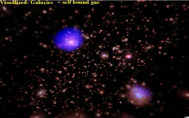
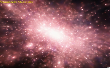
Figure 4: Sequence of ray-tracing of the internal structure of a galaxy cluster (Dolag et al., in preparation). Here different components, such as diffuse gas, stars in individual member galaxies, gas bound in such galaxies and diffuse stars within the galaxy cluster are used in different combinations for producing the images. Such visualisations can give unique impressions of the structure and the dynamical interplay between these different components as predicted in such high resolution “zoomed” simulations. Here a special colour scheme has been used, to produce colours similar to those in the well-known image of the Orion nebula, obtained by the Hubble Space Telescope. The movie can be downloaded from http://www.mpa-garching.mpg.de/galform/data_vis/index.shtml#movie9.

In some cases, even a flight through a non-evolving representation of cosmological structures can be very enlightening. To optimise such a case, Splotch allows to read the geometrical setup (i.e. the camera position $\vec{c}$, the look-at point $\vec{l}$ and the sky vector $\vec{s}$) from a plain ASCII file. Thereby, it produces one frame for every entry in the file, without having to reload the cosmological simulation every time. This can be quite handy, especially when the simulation data are huge (several GB or more). It is also useful to pre-process the data to emphasise different aspects of a cosmological simulation. For example, figure 4 shows a flight through an extremely highly resolved galaxy cluster taken from Dolag et al., in preparation (more than 25 million particles within the cluster). Here, different components have been separated in a post-processing step using SUBFIND (Springel et al., 2001) to separate diffuse and self-bound substructures within the galaxy cluster. The movie starts from showing the structures in and around the hot atmosphere of a galaxy cluster. After zooming into the cluster, the camera path follows an elliptical orbit around the center. Prominent structure within the hot plasma becomes visible. Changes of the saturation and colour settings reveal different structures at different scales and their interactions. Some of the sub-structures inside the cluster are able to maintain a self-bound atmosphere for a while (shown in light blue). The population of free-floating stars, which originates from destroyed galaxies, shows prominent stripes as imprints of the orbits of the former galaxies they belonged to. Despite such destruction, more than one thousand of individual galaxies can still be identified within the cluster, forming new stars in their centers (shown in dark blue). Only a small number of these are still maintaining a hot, self-bound atmosphere (shown in light blue). In the zoom-out all the stars formed within the simulation are shown. The text and some visual blending effects are produced by a post-processing step. This animation can also be downloaded from http://www.mpa-garching.mpg.de/galform/data_vis/index.shtml#movie9.

4 The 4D Universe

The visual rendering of the universe and its evolution can represent a spectacular approach toward the intuitive explanation of the complex phenomena that are at the bases of our incredibly fascinating theory of cosmology, for both scientists and common people. Unfortunately, an effective implementation of this approach is extremely challenging, and it often leads to scientifically non-rigorous or even misleading realisations. Even the most rigorous approaches lead to incomplete or partial results, due to the difficulties in effectively give a graphic representation of the three-dimensional space in which matter, stars and galaxies are born, move, evolve and interact leading to the wonderful texture that we can observe in the sky.

We have exploited an unprecedented combination of numerical modelling, astronomical observational data and Splotch-based rendering to create a 4D reconstruction of the universe, as described by the commonly accepted model. The full 3D volumetric representation is provided by the adoption of the stereographic rendering approach, according to the technique described below.

Even more challenging, the fourth dimension, time, is obtained by describing the dynamics and the behaviour of cosmological structures from their birth to the present epoch, using the results of state-of-the-art computer simulations.

The final outcome is an animation displaying a flight through a volume representative of the universe, following its evolution. In the first part of the animation the focus is on the complex architecture of filaments and sheets which define the cosmological large-scale structure. We then concentrate on a cluster of galaxies, and the thousands of small objects, the galaxies, which compose it. Finally, we zoom in, showing the fascinating structures of a spiral galaxy, as we belive our own Milky Way is like. The result of this effort will be displayed in the Virtual Reality facility of the brand new Turin Planetarium.

In the rest of this section, we will describe the main steps in the realisation of the 4D Universe animation.

4.1 Splotch usage and stereographic rendering

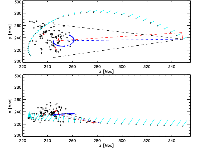
Figure 5: The geometrical setup of the camera path for the cosmological movie in two projections to describe the 3D setup. The diamonds mark the positions of the largest cosmological objects in the simulation volume, the black plus symbols mark the position of the camera with the sky vector $\vec{s}$ attached in light blue. The dark blue plus symbols show the look-at position $\vec{l}$. Both are shown tracing their movement for the full movie sequence, plotting only every hundredth position. For the first frame, the view vector $\vec{v}$ is shown as blue dashed line, encompassed by the black dashed lines marking the visible region defined by the field-of-view angle $\varphi$. The red line marks the right vector $\vec{r}$ and the red dashed vector marks the view vector for the right eye. Note that here a (unphysically large) value of $\beta=6$ was used for visualisation purpose.

The realisation of such a complex visualisation project required to properly fine-tune the usage of Splotch. Colours, transparencies, smoothing lengths adapt to the represented environment and objects, which continuosly change following the evolution of cosmological structures and the movements of the camera.

The movie supports stereographic visualisation. Therefore two different realisations of the movie, one for each eye, must be produced. This is accomplished by generating two different camera paths and creating the frame sequence according to each path. The two paths are calculated as follows.

As described before, the geometry for the rendering is given by three vectors: the camera position $\vec{c}$, the look-at point $\vec{l}$, and the sky vector $\vec{s}$. The first two vectors define the viewing vector $\vec{v}=\vec{l}-\vec{c}$. In general, the sky vector $\vec{s}$ does not have to be orthogonal to the view vector $\vec{l}$ to be used in Splotch. However, a simple projection

$$\vec{S}=\vec{s}-{\mathrm{c}os}(\alpha)\,\vec{v}\,\frac{|\vec{s}|}{|\vec{v}|}$$ (4)

can be used to obtain the its orthogonal part $\vec{S}$, where $\alpha$ is the angle between the sky vector $\vec{s}$ and the view vector $\vec{v}$, which can be obtained by the classical formula

$${\mathrm{c}os}(\alpha)=\frac{\vec{v}\cdot\vec{s}}{|\vec{v}|\,|\vec{s}|}.$$ (5)

For stereoscopic projection, the same scene is re-rendered from the position of the second eye calculated as follows. If we parameterise the position of the right eye by a separation angle $\beta$, the new camera position for the right eye $\vec{C}$ can be obtained easily

$$\vec{C}=\vec{c}+\frac{\vec{r}}{|\vec{r}|}\,\frac{\beta\,2\pi}{360}\,|\vec{v}|,$$ (6)

whereas the vector $\vec{r}$ can be simply obtained by the cross product $\vec{r}=\vec{S}\times\vec{v}$ defining the right direction. Afterwards, the two images for the different eye positions can be combined to be used in stereoscopic devices. For the movie we used values between $0.15$ and $0.2$ for $\beta$, depending on the final device used. Figure 5 shows the geometrical setup for the cosmological part of the 4D universe movie. It shows the relation between the different involved vectors as well.

4.2 The Big Bang

The representation of the first few instants after the Big Bang is an incredibly difficult task. Nothing that we can conceive is able to properly describe what happened in that initial time frame. We have adopted an abstract geometric representation, in which a spherical symmetric mesh represents the expanding space-time (see figure 6). One of the cells of this mesh is selected and represents the sample volume where the subsequent stages, based on the simulated data, take place.

Since Splotch renders only point-like data, this part of the movie, based on polygonal data, has been modeled and rendered using a commercial 3d graphic package: Autodesk 3DStudio Max.

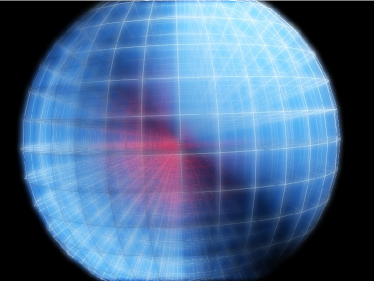
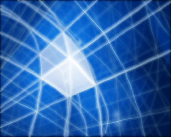
Figure 6: Representation of the geometry of the space-time in the very first instants of the Big Bang.

4.3 The evolution of the Universe

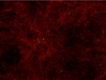
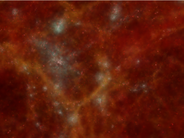
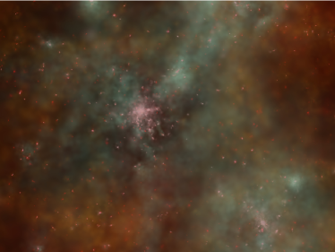
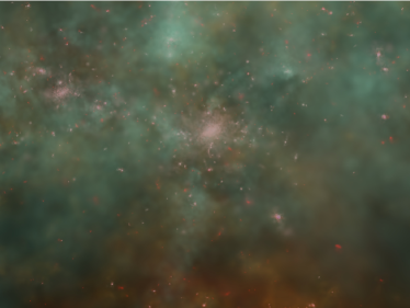
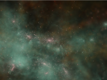
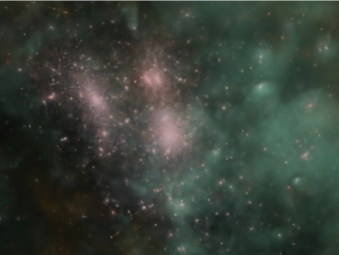
Figure 7: Sequence of ray-tracing a flight through the evolving structure from a cosmological simulation. Here, different components, gas and stars, are visualised together, but using two different colour tables. The colour table for the gas is specially trimmed to become transparent at high densities, so that stars inside the forming gaseous atmosphere are visible. A compressed version of the 4D Universe movie can be obtained from http://www.mpa-garching.mpg.de/galform/data_vis/index.shtml#movie11.

For a project like the 4D Universe, it is necessary to create the images making use of data from an extremely high resolution simulation. We used a simulation of a large cosmic structure which connects 4 very massive galaxy clusters (see Dolag et al., 2006). The high resolution region in this simulation is more than one order of magnitude larger than that of the simulations of individual clusters presented in section 3. Figure 7 shows some frames extracted from the cosmological part of the movie. The flight through an evolving cosmic structure starts at early times (the so-called dark ages), where the matter in the universe is in a cold and neutral state. First objects collapse and form the first proto-galaxies embedded in a heated atmosphere, hosting the first stars and quasars (QSOs). The high energy light from those stars/QSOs heats and ionises the material in the universe. Although cosmological simulations cannot take this effect into account self-consistently, the adoption of a time-dependent background radiation field mimics the effects of re-heating the universe and reveals the fine, filamentary structures formed until that point. Larger and larger structures form within a long and violent process of merging of smaller structures leading to the formation of the galaxy clusters, still connected to each other by filamentary structures. At the end, the movie zooms into a spiral galaxy, similar to what we expect the Milky Way to look like, for a final fly-by. In this case the galaxy is artificially constructed from an astronomical image (as described in the next section), as it is still impossible to obtain such detailed and realistic galaxies directly within cosmological simulations.

4.4 The Galaxy

Galaxies, and in particular spiral galaxies, are amongst the most spectacular objects in the universe. For many galaxies, high resolution images have been caught (e.g. by the Hubble Space Telescope, http://heritage.stsci.edu/2005/12a/big.html), which provide a detailed description of their structure and morphological features.

However, for the sake of 4D visualisation, several difficulties must be overcome. Firstly, even the ultimate cosmological simulations fail to produce spiral galaxies as detailed as we observe them in the real world. This is due to actual limitations in resolution and lack of possibility to properly include all key physical processes important to form a spiral galaxy from first principles. Secondly, any observation of a galaxy reflects only 2D, projected images of the object. The detailed 3D shape of the galaxy is unknown. Furthermore, no time evolution can be observed, the dynamical time-scale being hundreds of millions of years. We solved these problems by a proper modelling of the galaxy and its evolution, based on observations combined with theoretical predictions of their dynamics.

The galaxy model is built in two main steps: the reconstruction of the 3D geometry (based on the Galaxian code) and the time evolution (based on the EvolveGalaxy code).

Step 1: the Galaxian code

In order to reconstruct the spatial distribution of the basic matter components of the galaxy (the disk, with stars and gas, the bulge and the globular cluster) we have developed a code called Galaxian, which works as follows.

$\bullet$ A specific galaxy is selected and its high resolution image converted to a raw format (more easily readable by our code) with a depth of 256 colours. This is the main data input of the code. For the planetarium movie, we have chosen the M51a spiral galaxy, also known as the Whirlpool Galaxy.

$\bullet$ In order to generate a 3D distribution close to that of the gas distributed in the galaxy, we define for each image’s pixel a point, with z-coordinate randomly extracted from a Gaussian distribution centered on the galactic plane, setting $\sigma_{z}$ much smaller than the galaxy radius. In this way we imitate the planar geometry of the spiral galaxy. Around each point, a cloud of $N$ points is generated with spherical symmetry. The points get the colour of the pixel in which it falls in. This permits to define a volumetric point distribution, avoiding, at the same time, to get a pixelled aspect: points uniformly distributed along $z$ on the same pixel have the same colour. This would lead to the emergence of un-physical monochromatic columns.

$\bullet$ Disk stars are represented by points with random positions covering the whole galaxy map. The three coordinates are generated following a Gaussian probability function with $\sigma_{x}\sim\sigma_{y}\gg\sigma_{z}$ in order to get an oblate spheroidal distribution. Bulge stars are generated at the center of the galaxy with a quasi–spherical distribution.

$\bullet$ Finally, a spherically symmetric distribution of globular clusters is generated around the galaxy. Each globular cluster accounts for several thousands (the precise number being random) of stars.

Step 2: the EvolveGalaxy code

Giving a self-consistent numerical description of the galaxy dynamics is an outstanding task, which is only marginally accomplished by the most advanced and expensive numerical simulations. For our pourposes, a simpler approach is sufficient. Such an approach is implemented in the EvolveGalaxy code, according to the following steps.

$\bullet$ A typical galaxy rotation curve is used to make all the gas and stars points on the disk rotate, according to the differential rotation law. This results in a purely kinematic approach (no dynamics considered).

$\bullet$ The stars in the bulge and in the globular clusters rotate around the galaxy center, each with its own constant velocity, calculated in order to balance the gravitational attraction of the matter distributed inside the orbit.

$\bullet$ Equations of motion af the disk points are integrated using a simple first order integration method. Due to the kinematic approach and the amplification of numerical errors, the description is acceptable for a limited time range only. After a few hundred million years, the point distribution becomes meaningless and the simulation must be stopped.

$\bullet$ At proper time intervals, the point distribution can be rendered calling the Splotch function directly from inside EvolveGalaxy. The code can be used on multiprocessor computers, making each computing element calculating a different fraction of the whole time evolution, strongly accelerating the rendering process. Figure 8 shows the result of this process. A compressed version of the 4D Universe movie can be obtained from http://www.mpa-garching.mpg.de/galform/data_vis/index.shtml#movie11. Note that in this version, the galaxy was implanted directly within the cosmological simulation and both the large scale structure as well as the galaxy were rendered at once. Here all geometrical calculations as well as the position data where adapted to be double precision to handle the large dynamical range between the galaxy and the cosmological structure. Therefore the part of zoomin onto and out of the galaxy, as well as the background structure when flying around the galaxy appear self consistent within the visualization.

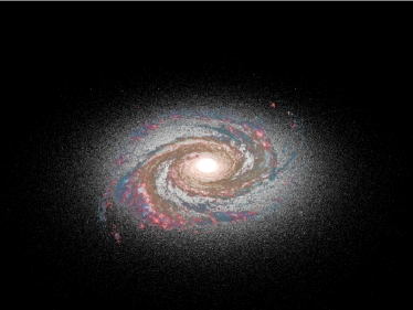
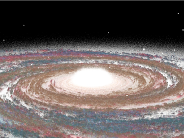
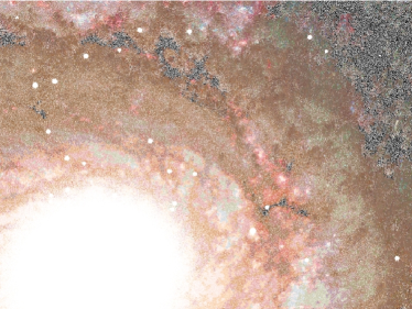
Figure 8: Sequence of ray-tracing a flight through a reconstructed galaxy planted into the cosmological simulation. Here the different components, gas in the disk, stars in the disk, bulge and globular clusters are visualised together. However, every gas and star particle has a vector array directly reflecting its RGB colours, which is used instead of the colour look-up table. The reconstruction is based on the colours composed from a real, optical observation (see text for details). The particles of the galaxy are added to the cosmological simulation and ray-traced in one shot, so that consistent movements of the galaxy and the background is accomplished. A compressed version of the 4D Universe movie can be obtained from http://www.mpa-garching.mpg.de/galform/data_vis/index.shtml#movie11.

5 Conclusions

Visualisation is one of the most effective techniques to explore and present scientific data, understanding at a glance its basic features and properties. Proper graphical solutions must be developed and exploited in order to fully achieve such objective. Such solutions can change according to the target users, depending, for example, whether professionals or common people are addressed. Moreover, different application fields can have specific requirements and different data sets can have peculiarities which need to be treated with a suitable approach.

Furthermore, the software must be able to face the major challenge represented by present time scientific datasets: the huge data volume. Visualisation tools have to be able to manipulate Gbytes of data at once, producing the result in an acceptable time. The algorithm must be tuned on the data in order to get the best possible performance. 64bit architectures, large memories and multi-processor systems have to be supported and exploited in order to handle such extraordinary data processing efforts.

In this paper, we have shown how the Splotch software can be adapted to a variety of different applications in astronomy, ranging from professional usage to divulgation and outreach contents production. For point-like data sets, Splotch meets all the previous requirements, adding the further advantage of being open source, flexible and easily extensible. It can be used both as a stand-alone application and as a library function, callable from inside the simulation code.

Splotch was successfully used to produce a stereographic movie for the Turin Planetarium. The movie has the ambitious goal of describing the birth and the evolution of the universe, exploiting actual cosmological numerical simulations, observations and models. Therefore it helps to give the general public an exceptional insight in our understanding of the world on its largest scales.

As a side product of the increased complexity of the physical systems captured by state of the art, cosmological simulations, visualisations of them are extremely attractive for the public and start to reach the state where they are of comparable beauty than real observations, which traditionally reflected the extremely attractive nature of astronomy.

References

- (1)
- Borgani et al. (2006) Borgani S, Dolag K, Murante G, Cheng L M, Springel V, Diaferio A, Moscardini L, Tormen G, Tornatore L and Tozzi P 2006 MNRAS 367, 1641–1654.
- Borgani and Guzzo (2001) Borgani S and Guzzo L 2001 Nature 409, 39–45.
- Borgani et al. (2004) Borgani S, Murante G, Springel V, Diaferio A, Dolag K, Moscardini L, Tormen G, Tornatore L and Tozzi P 2004 MNRAS 348, 1078–1096.
- Dolag et al. (2008) Dolag K, Borgani S, Schindler S, Diaferio A and Bykov A M 2008 Space Science Reviews 134, 229–268.
- Dolag et al. (2006) Dolag K, Meneghetti M, Moscardini L, Rasia E and Bonaldi A 2006 MNRAS 370, 656–672.
- Gingold and Monaghan (1977) Gingold R A and Monaghan J J 1977 MNRAS 181, 375–389.
- Lucy (1977) Lucy L B 1977 AJ 82, 1013–1024.
- Monaghan and Lattanzio (1985) Monaghan J J and Lattanzio J C 1985 A&A 149, 135–143.
- Shu (1991) Shu F 1991 Physics of Astrophysics: Volume I Radiation Published by University Science Books, 648 Broadway, Suite 902, New York, NY 10012, 1991.
- Springel (2005) Springel V 2005 MNRAS 364, 1105–1134.
- Springel et al. (2001) Springel V, White S D M, Tormen G and Kauffmann G 2001 MNRAS 328, 726–750.