Optimal approximation of harmonic growth clusters by orthogonal polynomials

Abstract

Interface dynamics in two-dimensional systems with a maximal number of conservation laws gives an accurate theoretical model for many physical processes, from the hydrodynamics of immiscible, viscous flows (zero surface-tension limit of Hele-Shaw flows, Hele-Shaw ), to the granular dynamics of hard spheres Jag-Nag , and even diffusion-limited aggregation Halsey . Although a complete solution for the continuum case exists Krichever-Mineev-Weinstein_et_al ; MWZ , efficient approximations of the boundary evolution are very useful due to their practical applications Put02 . In this article, the approximation scheme based on orthogonal polynomials with a deformed Gaussian kernel Teodorescu04 is discussed, as well as relations to potential theory.

Introduction –

A large class of two-dimensional processes, both deterministic and stochastic, have been mapped to a powerful mathematical model known as harmonic (or Laplacian) growth Bear ; CahnHill ; DLA81 ; Gollub ; Glicksman ; Howison86 ; KruSeg ; Langer ; Nakaya . In this model, a domain $D_{+}(t_{0})$ grows in time $t$, i.e. its normalized area $t_{0}=\pi^{-1}\int_{D_{+}}dxdy$ (areas in units of $\pi$ throughout) has a linear dependence $t_{0}=Qt$, with $Q$ the pumping rate.

This prescription is obtained as a consequence of the complete formulation as an exterior problem: if $\Gamma$ represents the boundary of $D_{+}$ and $D_{-}$ its complement, we seek the harmonic field $p$ (which may represent pressure, concentration, etc) and the velocity field $\vec{v}$, such that:

$$\left\{\begin{array}[]{lcl}v_{n}=-\partial_{n}p,&p=0&\mbox{on}\,\,\Gamma,\\ \vec{v}=-\vec{\nabla}p,&\Delta p=0&\mbox{on}\,\,D_{-},\\ p\sim-\log|z|,&\,\,z\to\infty&\in D_{-}\end{array}\right.$$ (1)

with $v_{n},\partial_{n}p$ their normal components on $\Gamma$, respectively.

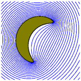
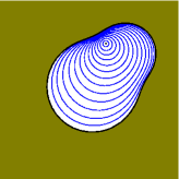
Figure 1: Simply connected droplets and equipotential lines for the interior and the exterior domains.

An equivalent formulation of the interior problem was studied by S. Richardson Richardson72 , where the roles of exterior and interior domains are interchanged: $p$ is harmonic inside up to a finite number of isolated logarithmic singularities (sources and sinks). Assume for simplicity a single point source at the origin $z=0$ with pumping rate $Q$, or, in terms of the pressure $p$, $\Delta p=\frac{Q}{2\pi}\,\delta^{2}(z)$. Richardson proved that for any function $h\in L^{1}(D_{+})$ harmonic in a neighborhood of $D_{+}$ we have

$$\frac{d\langle h\rangle_{+}}{dt}=Qh(0),$$ (2)

where $\langle h\rangle_{+}=\int_{D_{+}(t)}h(z)dxdy$. Therefore, taking $h(z)=z^{k}$ we have that the interior harmonic moments

$$v_{k}=\frac{1}{\pi}\int_{D_{+}(t)}\,z^{k}\,dx\,dy,\qquad k=1,2,\ldots$$ (3)

are preserved while the area grows linearly with $t$.

Mapping the interior problem by means of a simple coordinate change $\tilde{z}=1/z$ and changing the source to a sink ($Q\to-Q$) implies that in the original exterior problem for $D_{-}$ , $0\in D_{-}$, the exterior harmonic moments

$$t_{k}=-\frac{1}{k\pi}\int_{D_{-}(t)}\,z^{-k}\,dx\,dy,\qquad k=1,2,\ldots$$ (4)

(the interior moments of $D_{-}$ now) are preserved by the evolution and $dt_{0}/dt=Q$ Varchenko/Etingof:1992 , and we set $Q=1$.

For a simply connected droplet $D_{+}$, the solution of the problem is easily expressed through the conformal map taking the exterior of the unit disk $|\zeta|>1$ univalently onto $D_{-}$, and matching the points at infinity,

$$z=f(\zeta)\equiv r\zeta+\sum_{k=0}^{\infty}u_{k}\zeta^{-k},\quad r>0,$$ (5)

with respect to which the pressure and normal component of boundary velocity read

$$p(z)=-\log|f^{-1}(z)|,\quad v_{n}=|\partial_{z}f^{-1}(z)|.$$ (6)

As shown in MWZ , conservation of exterior harmonic moments is equivalent to the statement that there is a canonical transformation from the variables $z,z^{\sharp}$,

$$z=f(\zeta),\quad z^{\sharp}=\overline{f}(\zeta^{-1}),$$ (7)

to the variables $t_{0},\log\zeta$, i.e. $\zeta\left[\frac{\partial z}{\partial\zeta}\frac{\partial z^{\sharp}}{\partial t_{0}}-\frac{z^{\sharp}}{\partial\zeta}\frac{\partial z}{\partial t_{0}}\right]=1.$ We note the alternative formulation $dz\wedge dz^{\sharp}=d\log\zeta\wedge dt_{0}.$

In this paper, we describe an optimal approximation procedure for the boundary $\Gamma(t)$, as well as for the Cauchy transform of $D_{+}$,

$$C_{D_{+}}(z)=\frac{1}{\pi}\int_{D_{+}}\frac{dx^{\prime}dy^{\prime}}{z-z^{\prime}},\quad z^{\prime}=x^{\prime}+iy^{\prime},\,\,z\in D_{-}.$$ (8)

An example –

A superficial analysis of the model described here would lead to the conclusion that, given the integrability of the system, specifying a set of exterior harmonic moments $\{t_{k}\}$ at a given, initial area $T_{0}$, should yield a solution for $t_{0}>T_{0}$ without major analytical difficulties. In reality, reconstructing the conformal map (5) which corresponds to the data $T_{0},\{t_{k}\}$ is typically a very difficult problem. There are few known correpondences, between classes of moments $\{t_{k}\}$ and classes of shapes (5) (see Teodorescu04 for examples). An illustrative case occurs when the exterior harmonic moments form a simple sequence

$$t_{k}=-\frac{\beta}{k}a^{-k}\qquad k=1,2,\dots,$$ (9)

where $\beta\in\mathbb{R}^{+}$ and $a\in\mathbb{C}\setminus\{0\}$ are given parameters. Defining two radii

$$R_{1}=\sqrt{\beta},\qquad R_{2}=\sqrt{\frac{1+2\beta}{2}},$$ (10)

we have two completely different cases: if $|a|+R_{1}\leq R_{2}$ then we have a doubly connected domain bounded by circles and for $|a|+R_{1}>R_{2}$ the domain is simply connected given by an exterior conformal map of the form

$$f(\zeta)=r\zeta+u+\frac{v}{\zeta-A},\qquad r>0,\,\,|A|<1,$$ (11)

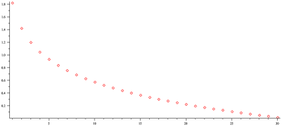
Figure 5: The Kullback-Leibler divergence of ${\rho_{n}^{(N)}(z)}$ with respect to the harmonic measure.

(see FIG. 5). The parameters of $f(\zeta)$ are related to the deformation parameters as follows: setting $u=v/A$,

$$\left\{\begin{array}[]{rcl}\displaystyle\beta&=&\displaystyle t_{0}-r^{2}+\frac{r\bar{v}}{{\bar{A}}^{2}},\\ a&=&\displaystyle\frac{r}{\bar{A}}+\frac{v}{A}+\frac{v\bar{A}}{1-|A|^{2}},\end{array}\right.$$ (12)

where $t_{0}=r^{2}-|v|^{2}/(1-|A|^{2})^{2}$ is the area. If $|a|+R_{1}>R_{2}$ then the above equations have a unique solution for $r,v$ and $A$ in terms of $\beta$ and $a$.

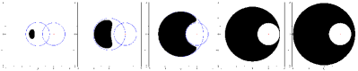
Figure 2: Laplacian growth for the exterior moments (9).

Domain approximation via orthogonal polynomials–

The fact that, even for a rather simple shape (11) the correspondence (12) is quite intricate shows the need for, and practical value of, efficient approximation methods. To that end, we define the following family of orthogonal polynomials: consider the domain specified by the exterior harmonic moments $\{t_{k}\}$ and $t_{0}$. The function defined in a neighborhood of the origin by

$$V(z)=\sum_{k\geq 1}t_{k}z^{k},\quad z\to 0,$$ (13)

is preserved by the harmonic growth. Now consider the function $W(z)=|z|^{2}-2\Re V(z)$, which we label confining potential, and suppose that

$$\int_{\mathbb{C}}|z|^{n}e^{-NW(z)}d^{2}z<\infty\qquad n=0,1,2,\dots$$

for all for values of the scaling parameter $N>0$. For fixed $N$, the orthogonal polynomials $\{P^{(N)}_{n}(z)\}$ of the weight function $e^{-NW(z)}$ are defined by

$$\int_{\mathbb{C}}P^{(N)}_{n}(z)\overline{P^{(N)}_{m}(z)}e^{-NW(z)}d^{2}z=\delta_{nm}.$$ (14)

The approximation method presented in this work is based on the following statement: as

$$n\to\infty,\quad N\to\infty,\quad\frac{n}{N}\to t_{0},$$ (15)

the weighted polynomials $|P^{(N)}_{n}(z)|^{2}e^{-NW(z)}$ (which we denote by $\rho_{n}^{(N)}(z)$ in the following) converge to the conformal measure of the domain $D_{+}(t)$, with support $\Gamma(t)$:

$$\rho_{n}^{(N)}(z)=|\partial_{z}f^{-1}(z)|\left[1+O\left(\frac{1}{N}\right)\right],\,\,n,N\to\infty.$$ (16)

The proof of this result appeared first in Teodorescu04 . We do not repeat the entire argument, as it would require too much space, but recollect the main ideas: starting from the differential equations satisfied by the weighted functions $\psi_{n}(z)=P_{n}^{(N)}(z)e^{-NW(z)/2}$, with respect to variables $n/N$ and $z$, we integrate perturbatively in powers of $N^{-1}$, and obtain the expression (Teodorescu04 , equation (76)):

$$\psi(z)\sim\sqrt{[f^{-1}(z)]^{\prime}}\exp\left[N\left(-\frac{|z|^{2}}{2}+\Re\int^{z}S(\zeta)d\zeta\right)\right],$$

where the Schwarz function $S(z)$ is defined by the identity $S(z)=\bar{z},z\in\Gamma$. It is known to have the expansion

$$S(z)=V^{\prime}(z)+\frac{1}{\pi}\int_{D_{+}}\frac{dx^{\prime}dy^{\prime}}{z-z^{\prime}},\quad z\to\infty$$ (17)

Since the exponent in the asymptotic expression of $\psi(z)$ vanishes on the boundary $\Gamma$ and gives a Gaussian decay away from it, the weighted polynomials $\rho_{n}^{(N)}(z)$ are described, in the $n,N\to\infty$ limit, by the conformal measure (16). However, this asymptotic result says very little about the behavior of $\rho_{n}^{(N)}(z)$ for finite values of $n,N$.

In the remainder of this paper, we present numerical evidence for the convergence properties of $\rho_{n}^{(N)}(z)$ at finite values of their order. We show that the agreement between $\rho_{n}^{(N)}(z)$ and $|[f^{-1}(z)]^{\prime}|$ is excellent for values of $n$ as little as $n=20$, and present potential applications of this property. One obvious consequence is related to reconstruction algorithms of domains in this class: assume that the Schwarz function of the domain $D_{+}$ has a branch cut on $\gamma\in D_{+}$, with real, positive jump function $\rho_{s}(z)$. Obviously, this may include the case of meromorphic functions with poles in $z_{p}\in D_{+}$, for which $\rho_{s}(z)=\sum_{p}a_{p}\delta(z-z_{p})$. Then from the asymptotic result

$$\frac{1}{N}\log|\rho_{N}^{(N)}(z)|\to W(z)+\frac{1}{\pi}\int_{D_{+}}\log|z-z^{\prime}|^{2}dx^{\prime}dy^{\prime},$$ (18)

it follows immediately that the asymptotic distribution of zeros of the orthogonal polynomials converges to $\rho_{s}(z)$:

$$\lim_{N\to\infty}\frac{1}{N}\sum_{i=1}^{N}\log|z-z_{i}|^{2}=\int_{\gamma}\rho_{s}(z^{\prime})\log|z-z^{\prime}|^{2}dz^{\prime}.$$ (19)

In a forthcoming publication Ed_Ferenc_Razvan , we will give detailed proofs of (16, 19). In this Letter, we provide a thorough numerical analysis supporting the asymptotic results.

Simulations and numerical study –

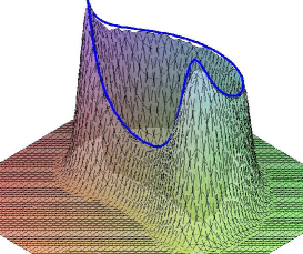
Figure 3: Localization for the density for $n=20$ and the conformal measure.

Let $t_{0}$ and the exterior harmonic moments be given through the potential $V(z)$. To fix the scaling limit, let $N(n)=n/t_{0}$. For fixed $n$, we have to calculate the entries of the Gram matrix

$$g^{(n)}_{ij}=\int_{\mathbb{C}}z^{i}{\bar{z}}^{j}e^{-n/t_{0}W(z)}d^{2}z\quad i,j=0,\dots,n.$$ (20)

For potentials $W(z)$ that are converging rapidly enough to infinity as $|z|\to\infty$, the exponentially decaying weight makes the planar numerical integration a feasible task. The stabilized Gram-Schmidt Algorithm provides the orthogonal polynomials $P_{n,N}(z)$, which is known to be very sensitive to the accuracy of the Gram matrix and thus requires very precise computation of $\{g^{(n)}_{ij}\}$ . Then the density $\rho_{n}^{(N)}(z)$ is obtained from the polynomial $P^{(N)}_{n}(z)$.

Of course, the usefulness of this approximation scheme relies on the rapidity of the convergence in (16), which may not seem to be very promising. However, our numerical experiment (FIG. 3) shows that in the example (9) above the “shape” of the conformal measure (the blue curve) is recovered very accurately by the weighted polynomial density of a degree as low as $n=20$.

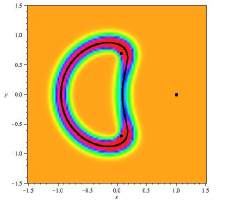
Figure 4: Density plot and contour plot of the localized density

To illustrate the speed of convergence in (16), the Kullback-Leibler divergence or relative entropy of ${\rho_{n}^{(N)}(z)}$ with respect to the harmonic measure, given by

$$\frac{1}{2\pi}\int_{0}^{2\pi}\left(\log{\frac{1}{|f^{\prime}(e^{i\theta})|}}-\log{\rho_{n}^{(N)}(f(e^{i\theta}))}\right)d\theta,$$ (21)

is calculated and plotted on the figure below.

The asymptotic behaviour of the zeroes of orthogonal polynomials in the scaling limit (15) was also investigated in the particular case (9). Since $f(\zeta)$ is a rational function of order two, the Cauchy transform $C_{D_{+}}(z)$ (8) in the exterior domain $D_{-}$ satisfies a quadratic equation

$$A(z)y^{2}+B(z)y+C(z)=0,$$

with rational coefficients in $z$ depending on the parameters of $f(\zeta)$. As an algebraic function, $C_{D_{+}}(z)$ can be analytically continued on a plane with a branch cut connecting up the branchpoints

$$z_{1,2}=\frac{v}{A}+Ar\pm 2\sqrt{rv}$$ (22)

of the inverse mapping $f^{-1}(z)$. This “conjugate electric field” created by the uniformly charged domain $D_{+}$ is mimicked by the field generated by the normalized counting measure of the zeroes. However, these points seem to accumulate along some curve (as opposed to the equilibrium configuration in the presence of the background potential $W(z)$ – the so-called Fekete points – which are distributed asymptotically uniformly). Since the asymptotic zero distribution must be real and positive, the natural choice is dictated by the Sokhotski-Plemelj formula: the critical trajectory $\gamma$ is selected by the condition that the jump between the two solutions $y_{\pm}=(-B\pm\sqrt{B^{2}-4AC})/2A$ satisfies

$$\Re\left((y_{+}(z)-y_{-}(z))dz\right)=0.$$ (23)

The critical trajectory can be found by calculating

$$\Phi(z):=\Re\left[\int_{z_{1}}^{z}(y_{+}(w)-y_{-}(w))dw\right]$$ (24)

and then plotting the contour $\Phi(z)=0$. Three trajectories are emanating from each branchpoint: there are two trajectories that connect $z_{1}$ and $z_{2}$, and the one contained by the domain attracts the roots. As can be seen in FIG. 6, the distribution of zeros (for $n=50$) and the trajectory $\gamma$ are almost indistinguishable.

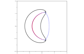
Figure 6: The critical trajectory and the zeroes for $n=50$.

Applications –

The method presented in this Letter allows to construct optimal approximations with high convergence rates for either the boundary or the branch cuts characterizing domains from the harmonic growth class. This may be used in a number of different situations; here we discuss two relevant examples:

$(i)$ an outstanding problem in viscous two-dimensional flows is formation of boundary singularities (cusps). They are known to occur for finite values of the normalized area $t_{0}$, and for many initial conditions Hohlov-Howison94 . For a particular class of such cusps, with local geometry given by the scaling $x^{2}\sim y^{2k+1},k=1,2,\ldots$, it is not possible to continue the evolution of the boundary beyond the cusp formation, and a weaker type of solution is required.

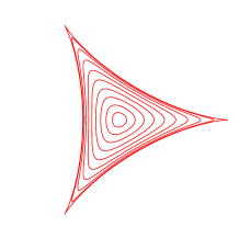
Figure 7: Singular shape as a result of Laplacian growth

The weak solution WT is based on the equivalence between the distribution of zeros of the orthogonal polynomials and the branch cut of the Schwarz function, (19). These two distributions generate the same Newtonian potential in $D_{-}$ as the uniform distribution on $D_{+}$ (real droplet), so they may be considered as equivalent solutions before singularity formation, FIG. 7. However, after a cusp is formed, smooth (uniform) solutions are not possible anymore, while the distribution of zeros of the polynomials remains well-defined. The conjecture is that this weak formulation will produce solutions which explain the famous fingering patterns observed in physical realizations of this model. This will be shown in a forthcoming publication, where the algorithm will be used to construct numerical solutions according to this prescription, and compare with real, physical patterns Sw .

$(ii)$ another practical application of the results presented in this Letter is an efficient algorithm for shape (boundary) reconstruction when the domain $D_{+}$ is given through the reduced data $t_{0},\{t_{k}\}$. For example, such (reduced) representations arise in satellite imaging data compression Put02 . Shape reconstruction algorithms are then needed to find the boundary $\Gamma$, given the set of moments $t_{0},\{t_{k}\}$, with particular emphasis on good convergence rates. Since the data $t_{0},\{t_{k}\}$ is sufficient for constructing the family of orthogonal polynomials $P^{(N)}_{n}$ introduced here, we have a boundary approximation algorithm which gives excellent results already at $n=20$.

References

- (1) H. S. S. Hele-Shaw. Nature, 58(1489):34–36, 1898.
- (2) X. Cheng, L. Xu, A. Patterson, H. M. Jaeger, and S. R. Nagel. Nature Physics, 4:234–237, March 2008.
- (3) T. C. Halsey. Physics Today, 53:36–41, 2000.
- (4) I. Krichever, M. Mineev-Weinstein, P. Wiegmann, and A. Zabrodin. Physica D, 198(1-2):1–28, 2004.
- (5) M. Mineev-Weinstein, P.B. Wiegmann, and A. Zabrodin. Physical Review Letters, 84:5106, 2000.
- (6) M. Putinar. Numer. Math., 93(1):131–152, 2002.
- (7) R. Teodorescu, E. Bettelheim, O. Agam, A. Zabrodin, and P. Wiegmann. Nuclear Phys. B, 704(3):407–444, 2005.
- (8) J. Bear. Dynamics of fluids in porous media. Elsevier (New York), 1972.
- (9) J. W. Cahn and J. E. Hilliard. The Journal of Chemical Physics, 28(2):258–267, 1958.
- (10) T. A. Witten and L. M. Sander. Phys. Rev. Lett., 47(19):1400–1403, 1981.
- (11) Y. Sawada, A. Dougherty, and J. P. Gollub. Phys. Rev. Lett., 56(12):1260–1263, 1986.
- (12) J. S. Langer and H. Müller-Krumbhaar. Phys. Rev. A, 27(1):499–514, 1983.
- (13) S. D. Howison. SIAM J. Appl. Math., 46(1):20–26, 1986.
- (14) M. D. Kruskal and H. Segur. Stud. Appl. Math., 85(2):129–181, 1991.
- (15) J. S. Langer. Phys. Rev. Lett., 44(15):1023–1026, 1980.
- (16) U. Nakaya. Snow Crystals. Harvard University Press., Cambridge, 1954.
- (17) S. Richardson. Journal of Fluid Mechanics, 56:609–618, 1972.
- (18) A.N. Varchenko and P.I. Etingof. Why the boundary of a round drop becomes a curve of order four. American Mathematical Society, 1992.
- (19) F Balogh, E Saff, and R Teodorescu. in preparation.
- (20) Y. E. Hohlov and S. D. Howison. Quart. Appl. Math., 51(4):777–789, 1993.
- (21) S-Y. Lee, R Teodorescu, and P Wiegmann, LA-UR 07-3622, unpublished.
- (22) E. Sharon, M. G. Moore, W. D. McCormick, and H. L. Swinney. Phys. Rev. Lett., 91(20):205504, 2003.