Feynman motives of banana graphs

Abstract.

We consider the infinite family of Feynman graphs known as the “banana graphs” and compute explicitly the classes of the corresponding graph hypersurfaces in the Grothendieck ring of varieties as well as their Chern–Schwartz–MacPherson classes, using the classical Cremona transformation and the dual graph, and a blowup formula for characteristic classes. We outline the interesting similarities between these operations and we give formulae for cones obtained by simple operations on graphs. We formulate a positivity conjecture for characteristic classes of graph hypersurfaces and discuss briefly the effect of passing to noncommutative spacetime.

1. Introduction

Since the extensive study of [15] revealed the systematic appearance of multiple zeta values as the result of Feynman diagram computations in perturbative quantum field theory, the question of finding a direct relation between Feynman diagrams and periods of motives has become a rich field of investigation. The formulation of Feynman integrals that seems most suitable for an algebro-geometric approach is the one involving Schwinger and Feynman parameters, as in that form the integral acquires directly an interpretation as a period of an algebraic variety, namely the complement of a hypersurface in a projective space constructed out of the combinatorial information of a graph. These graph hypersurfaces and the corresponding periods have been investigated in the algebro-geometric perspective in the recent work of Bloch–Esnault–Kreimer ([10], [11]) and more recently, from the point of view of Hodge theory, in [12] and [26]. In particular, the question of whether only motives of mixed Tate type would arise in the quantum field theory context is still unsolved. Despite the general result of [8], which shows that the graph hypersurfaces are general enough from the motivic point of view to generate the Grothendieck ring of varieties, the particular results of [15] and [11] point to the fact that, even though the varieties themselves are very general, the part of the cohomology that supports the period of interest to quantum field theory might still be of the mixed Tate form.

One complication involved in the algebro-geometric computations with graph hypersurfaces is the fact that these are typically singular, with a singular locus of small codimension. It becomes then an interesting question in itself to estimate how singular the graph hypersurfaces are, across certain families of Feynman graphs (the half open ladder graphs, the wheels with spokes, the banana graphs etc.). Since the main goal is to describe what happens at the motivic level, one wants to have invariants that detect how singular the hypersurface is and that are also somehow adapted to its decomposition in the Grothendieck ring of motives. In this paper we concentrate on a particular example and illustrate some general methods for computing such invariants based on the theory of characteristic classes of singular varieties.

Part of the purpose of the present paper is to familiarize physicists working in perturbative quantum field theory with some techniques of algebraic geometry that are useful in the analysis of graph hypersurfaces. Thus, we try as mush as possible to spell out everything in detail and recall the necessary background.

In §1, we begin by recalling the general form of the parametric Feynman integrals for a scalar field theory and the construction of the associated projective graph hypersurface. We recall the relation between the graph hypersurface of a planar graph and that of the dual graph via the standard Cremona transformation. We then present the specific example of the infinite family of “banana graphs”. We formulate a positivity conjecture for the characteristic classes of graph hypersurfaces.

For the convenience of the reader, we recall in §2 some general facts and results, both about the Grothendieck ring of varieties and motives, and about the theory of characteristic classes of singular algebraic varieties. We outline the similarities and differences between these constructions.

In §3 we give the explicit computation of the classes in the Grothendieck ring of the hypersurfaces of the banana graphs. We conclude with a general remark on the relation between the class of the hypersurface of a planar graph and that of a dual graph.

In §4 we obtain an explicit formula for the Chern–Schwartz–MacPherson classes of the hypersurfaces of the banana graphs. We first prove a general pullback formula for these classes, which is necessary in order to compute the contribution to the CSM class of the complement of the algebraic simplex in the graph hypersurface. The formula is then obtained by assembling the contribution of the intersection with the algebraic simplex and of its complement via inclusion–exclusion, as in the case of the classes in the Grothendieck ring.

We give then, in §5, a formula for the CSM classes of cones on hypersurfaces and use them to obtain formulae for graph hypersurfaces obtained from known one by simple operations on the graphs, such as doubling or splitting an edge, and attaching single-edge loops or trees to vertices.

Finally, in §6, we look at the deformations of ordinary $\phi^{4}$ theory to a noncommutative spacetime given by a Moyal space. We look at the ribbon graphs that correspond to the original banana graphs in this noncommutative quantum field theory. We explain the relation between the graph hypersurfaces of the noncommutative theory and of the original commutative one. We show by an explicit computation of CSM classes that in noncommutative QFT the positivity conjecture fails for non-planar ribbon graphs.

Acknowledgment. The first author is partially supported by NSA grant H98230-07-1-0024. The second author is partially supported by NSF grant DMS-0651925. We thank the Max–Planck–Institute and Florida State University, where part of this work was done. We also thank Abhijnan Rej for exchanges of numerical computations of CSM classes of graph hypersurfaces.

1.1. Parametric Feynman integrals

We briefly recall some well known facts (cf. §6-2-3 of [23], §18 of [9], and §6 of [27]) about the parametric form of Feynman integrals.

Given a scalar field theory with Lagrangian written in Euclidean signature as

(1.1) $${\mathcal{L}}(\phi)=\frac{1}{2}(\partial\phi)^{2}+\frac{m^{2}}{2}\phi^{2}+{\mathcal{L}}_{int}(\phi),$$

where the interaction part is a polynomial function of $\phi$, a one-particle-irreducible (1PI) Feynman graph of the theory is a connected graph $\Gamma$ which cannot be disconnected by removing a single edge, and with the following properties. All vertices in $V(\Gamma)$ have valence equal to the degree of one of the monomials in the Lagrangian. The set of edges $E(\Gamma)=E_{int}(\Gamma)\cup E_{ext}(\Gamma)$ consists of internal edges having two end vertices and external ones having only one vertex. A Feynman graph without external edges is called a vacuum bubble.

In perturbative quantum field theory, the Feynman integrals associated to the loop number expansion of the effective action for a scalar field theory are labeled by the 1PI Feynman graphs of the theory, each contributing a corresponding integral of the form

(1.2) $$U(\Gamma,p)=\frac{\Gamma(n-D\ell/2)}{(4\pi)^{\ell D/2}}\int_{[0,1]^{n}}\frac{\delta(1-\sum_{i}t_{i})}{\Psi_{\Gamma}(t)^{D/2}V_{\Gamma}(t,p)^{n-D\ell/2}}\,dt_{1}\cdots dt_{n}.$$

Here $n=\#E_{int}(\Gamma)$ is the number of internal edges of the graph $\Gamma$, $D\in{\mathbb{N}}$ is the spacetime dimension in which the scalar field theory is considered, and $\ell=b_{1}(\Gamma)$ is the number of loops in the graph, i.e. the rank of $H_{1}(\Gamma,{\mathbb{Z}})$. The function $\Psi_{\Gamma}$ is a polynomial of degree $\ell=b_{1}(\Gamma)$. It is given by the Kirchhoff polynomial

(1.3) $$\Psi_{\Gamma}(t)=\sum_{T\subset\Gamma}\prod_{e\notin E(T)}t_{e},$$

where the sum is over all the spanning trees $T$ of $\Gamma$. The function $V_{\Gamma}(t,p)$ is a rational function of the form

(1.4) $$V_{\Gamma}(t,p)=\frac{P_{\Gamma}(t,p)}{\Psi_{\Gamma}(t)},$$

where $P_{\Gamma}$ is a homogeneous polynomial of degree $\ell+1=b_{1}(\Gamma)+1$ of the form

(1.5) $$P_{\Gamma}(p,t)=\sum_{C\subset\Gamma}s_{C}\prod_{e\in C}t_{e},$$

Here the sum is over the cut-sets $C\subset\Gamma$, i.e. the collections of $b_{1}(\Gamma)+1$ edges that divide the graph $\Gamma$ in exactly two connected components $\Gamma_{1}\cup\Gamma_{2}$. The coefficient $s_{C}$ is a function of the external momenta attached to the vertices in either one of the two components

(1.6) $$s_{C}=\left(\sum_{v\in V(\Gamma_{1})}P_{v}\right)^{2}=\left(\sum_{v\in V(\Gamma_{2})}P_{v}\right)^{2},$$

where the $P_{v}$ are defined as

(1.7) $$P_{v}=\sum_{e\in E_{ext}(\Gamma),t(e)=v}p_{e},$$

where the $p_{e}$ are incoming external momenta attached to the external edges of $\Gamma$ and satisfying the conservation law

(1.8) $$\sum_{e\in E_{ext}(\Gamma)}p_{e}=0.$$

The divergence properties of the integral (1.2) can be estimated in terms of the “superficial degree of divergence”, which is measured by the quantity $n-D\ell/2$. The integral (1.2) is called logarithmically divergent when $n-D\ell/2=0$. The example of the banana graphs we concentrate on below has $n=\ell+1$, so that we find $n-D\ell/2=(1-D/2)\ell+1<0$ for $D>2$ and $\ell\geq 2$. In this case, we write the integral (1.2) in the form

(1.9) $$U(\Gamma,p)=\frac{\Gamma(n-D(n-1)/2)}{(4\pi)^{(n-1)D/2}}\int_{\sigma_{n}}\frac{P_{\Gamma}(p,t)^{-n+D(n-1)/2}\,\omega_{n}}{\Psi_{\Gamma}(t)^{n(-1+D/2)}},$$

where $\omega_{n}$ is the volume form and the domain of integration is the topological simplex

(1.10) $$\sigma_{n}=\{(t_{1},\ldots,t_{n})\in{\mathbb{R}}_{+}^{n}\,|\,\sum_{i}t_{i}=1\}.$$

The 1PI condition on Feynman graphs comes from the fact of considering the perturbative expansion of the effective action in quantum field theory, which reduces the combinatorics of graphs to just those that are connected and 1PI. In terms of the expression of the Feynman integral, the 1PI condition is reflected in the fact that only the propagators for internal edges appear. The parametric form we described above therefore depends on this assumption. However, for the algebro-geometric arguments that constitute the main content of this paper, the 1PI condition is not strictly necessary.

1.2. Feynman graphs, varieties, and periods

The graph polynomial $\Psi_{\Gamma}(t)$ of (1.3) also admits a description as determinant

(1.11) $$\Psi_{\Gamma}(t)=\det M_{\Gamma}(t)$$

of an $\ell\times\ell$-matrix $M_{\Gamma}(t)$ associated to the graph ([27], §3 and [9], §18), of the form

(1.12) $$(M_{\Gamma})_{kr}(t)=\sum_{i=1}^{n}t_{i}\eta_{ik}\eta_{ir},$$

where the $n\times\ell$-matrix $\eta_{ik}$ is defined in terms of the edges $e_{i}\in E(\Gamma)$ and a choice of a basis for the first homology group, $l_{k}\in H_{1}(\Gamma,{\mathbb{Z}})$, with $k=1,\ldots,\ell=b_{1}(\Gamma)$, by setting

(1.13) $$\eta_{ik}=\left\{\begin{array}[]{rl}+1&\text{edge $e_{i}\in$ loop $l_{k}$, same orientation}\\[5.69054pt] -1&\text{edge $e_{i}\in$ loop $l_{k}$, reverse orientation}\\[5.69054pt] 0&\text{otherwise,}\end{array}\right.$$

after choosing an orientation of the edges.

Notice how the result is independent of the choice of the orientation of the edges and of the choice of the basis of $H_{1}(\Gamma,{\mathbb{Z}})$. In fact, a change of orientation in a given edge results in a change of sign to one of the columns of the matrix $\eta_{ki}$, which is compensated by the change of sign in the corresponding row of the matrix $\eta_{ir}$, so that the determinant $\det M_{\Gamma}(t)$ is unaffected. Similarly, a change in the choice of the basis of $H_{1}(\Gamma,{\mathbb{Z}})$ has the effect of changing $M_{\Gamma}(t)\mapsto AM_{\Gamma}(t)A^{-1}$ for some $A\in{\rm GL}(\ell,{\mathbb{Z}})$ and the determinant is again unchanged.

The graph hypersurface $X_{\Gamma}$ is by definition the zero locus of the Kirchhoff polynomial,

(1.14) $$X_{\Gamma}=\{t=(t_{1}:\ldots:t_{n})\in{\mathbb{P}}^{n-1}\,|\,\Psi_{\Gamma}(t)=0\}.$$

Since $\Psi_{\Gamma}$ is homogeneous, it defines a hypersurface in projective space.

The domain of integration $\sigma_{n}$ defines a cycle in the relative homology $H_{n-1}({\mathbb{P}}^{n-1},\Sigma_{n})$, where $\Sigma_{n}$ is the algebraic simplex (the union of the coordinate hyperplanes, see (1.16) below). The Feynman integral (1.2), (1.9) then can be viewed ([11],[10]) as the evaluation of an algebraic cohomology class in $H^{n-1}({\mathbb{P}}^{n-1}\smallsetminus X_{\Gamma},\Sigma\smallsetminus\Sigma\cap X_{\Gamma})$ on the cycle defined by $\sigma_{n}$. In this sense, it can be viewed as the evaluation of a period of the algebraic variety given by the complement of the graph hypersurface. To understand the nature of this period, one is faced with two main problems. One is eliminating divergences (regularization and renormalization of Feynman integrals), and the other is understanding what kind of motives are involved in the part of the hypersurface complement ${\mathbb{P}}^{n-1}\smallsetminus X_{\Gamma}$ that is involved in the evaluation of the period, hence what kind of transcendental numbers one expects to find in the evaluation of the corresponding Feynman integrals. A detailed analysis of these problems was carried out in [11]. The examples we concentrate on in this paper are not especially interesting from the motivic point of view, since they are expressible in terms of pure Tate motives (cf. [10]), but they provide us with an infinite family of graphs for which all computations are completely explicit.

1.3. Dual graphs and Cremona transformation

In the case of planar graphs, there is an interesting relation between the hypersurface of the graph and the one of the dual graph. This will be especially useful in the explicit calculation we perform below in the special case of the banana graphs. We recall it here in the general case of arbitrary planar graphs.

The standard Cremona transformation of ${\mathbb{P}}^{n-1}$ is the map

(1.15) $${\mathcal{C}}:(t_{1}:\cdots:t_{n})\mapsto\left(\frac{1}{t_{1}}:\cdots:\frac{1}{t_{n}}\right).$$

This is a priori defined away from the algebraic simplex of coordinate axes

(1.16) $$\Sigma_{n}=\{(t_{1}:\cdots:t_{n})\in{\mathbb{P}}^{n-1}\,|\,\prod_{i}t_{i}=0\}\subset{\mathbb{P}}^{n-1},$$

though we see in Lemma 1.2 below that it is well defined also on the general point of $\Sigma_{n}$, its locus of indeterminacies being only the singularity subscheme of $\Sigma_{n}$.

Let ${\mathcal{G}}({\mathcal{C}})$ denote the closure of the graph of ${\mathcal{C}}$. Then ${\mathcal{G}}({\mathcal{C}})$ is a subvariety of ${\mathbb{P}}^{n-1}\times{\mathbb{P}}^{n-1}$ with projections

(1.17)

Lemma 1.1.

Using coordinates $(s_{1}:\cdots:s_{n})$ for the target ${\mathbb{P}}^{n-1}$, the graph ${\mathcal{G}}({\mathcal{C}})$ has equations

(1.18) $$t_{1}s_{1}=t_{2}s_{2}=\cdots=t_{n}s_{n}.$$

In particular, this describes ${\mathcal{G}}({\mathcal{C}})$ as a complete intersection of $n-1$ hypersurfaces in ${\mathbb{P}}^{n-1}\times{\mathbb{P}}^{n-1}$ with equations $t_{i}s_{i}=t_{n}s_{n}$, for $i=1,\dots,n-1$.

Proof.

The equations (1.18) clearly cut out ${\mathcal{G}}({\mathcal{C}})$ over the open set ${\mathcal{U}}\subset{\mathbb{P}}^{n}$ where all $t$-coordinates are nonzero. Since every component of a scheme defined by $n-1$ equations has codimension $\leq n-1$, it suffices to show that equations (1.18) define a set of codimension $>n-1$ over the complement of ${\mathcal{U}}$. Now assume that at least one of the $t$-coordinates equal $0$. Without loss of generality, suppose $t_{n}=0$. Intersecting with the locus defined by (1.18) determines the set with equations

$$t_{1}s_{1}=\dots=t_{n-1}s_{n-1}=t_{n}=0\quad,$$

which has codimension $n>n-1$, as promised. ∎

It is not hard to see that the variety ${\mathcal{G}}({\mathcal{C}})$ has singularities in codimension $3$. It is nonsingular for $n=2,3$, but singular for $n\geq 4$.

The open set ${\mathcal{U}}$ as above is the complement of the divisor $\Sigma_{n}$ of (1.16). The inverse image of $\Sigma_{n}$ in ${\mathcal{G}}({\mathcal{C}})$ can be described easily. It consists of the points

$$((t_{1}:\cdots:t_{n}),(s_{1}:\cdots:s_{n}))$$

such that

$$\{i\,|\,t_{i}=0\}\cup\{j\,|\,s_{j}=0\}=\{1,\dots,n\}\quad.$$

This locus consists of $2^{N}-2$ components of dimension $n-2$: one component for each nonempty proper subset $I$ of $\{1,\dots,n\}$. The component corresponding to $I$ is the set of points with $t_{i}=0$ for $i\in I$ and $s_{j}=0$ for $j\not\in I$.

The situation for $n=3$ is well represented by the famous picture of Figure 1. The three zero-dimensional strata of $\Sigma_{3}$ are blown up in ${\mathcal{G}}({\mathcal{C}})$ as we climb the diagram from the lower left to the top. The proper transforms of the one dimensional strata are blown down as we descend to the lower right. The horizontal rational map is an isomorphism between the complements of the triangles. The inverse image of $\Sigma_{3}$ consists of $2^{3}-2=6$ components, as expected.

Of course the situation is completely symmetric: the algebraic simplex (1.16) may be embedded in the target ${\mathbb{P}}^{n}$ as well (with equation $\prod_{i}s_{i}=0$). One has $\pi_{1}^{-1}(\Sigma_{n})=\pi_{2}^{-1}(\Sigma_{n})$.

Let ${\mathcal{S}}_{n}\subset{\mathbb{P}}^{n-1}$ be the subscheme defined by the ideal

(1.19) $${\mathcal{I}}_{{\mathcal{S}}_{n}}=(t_{1}\cdots t_{n-1},t_{1}\cdots t_{n-2}t_{n},\dots,t_{1}t_{3}\cdots t_{n},t_{2}\cdots t_{n}).$$

The scheme ${\mathcal{S}}_{n}$ is the singularity subscheme of the divisor with simple normal crossings $\Sigma_{n}$ of (1.16), given by the union of the coordinate hyperplanes. We can place ${\mathcal{S}}_{n}$ in both the source and target ${\mathbb{P}}^{n-1}$. Finally, let ${\mathcal{L}}$ be the hyperplane defined by the equation

(1.20) $${\mathcal{L}}=\{(t_{1}:\cdots:t_{n})\in{\mathbb{P}}^{n-1}\,|\,t_{1}+\cdots+t_{n}=0\}.$$

Figure 1. The Cremona transformation in the case $n=3$.

We then can make the following observations.

Lemma 1.2.

Let ${\mathcal{C}}$, ${\mathcal{G}}({\mathcal{C}})$, ${\mathcal{S}}_{n}$, and ${\mathcal{L}}$ be as above.

1. ${\mathcal{S}}_{n}$ is the subscheme of indeterminacies of the Cremona transformation ${\mathcal{C}}$.

2. $\pi_{1}:{\mathcal{G}}({\mathcal{C}})\to{\mathbb{P}}^{n-1}$ is the blow-up along ${\mathcal{S}}_{n}$.

3. ${\mathcal{L}}$ intersects every component of ${\mathcal{S}}_{n}$ transversely.

4. $\Sigma_{n}$ cuts out a divisor with simple normal crossings on ${\mathcal{L}}$.

Proof.

(1) Notice that the definition (1.15) of the Cremona transformation, which is a priori defined on the complement of $\Sigma_{n}$ still makes sense on the general point of $\Sigma_{n}$. Thus, the indeterminacies of the map (1.15) are contained in the singularity locus ${\mathcal{S}}_{n}$ of $\Sigma_{n}$ defined by (1.19). It consists in fact of all of ${\mathcal{S}}_{n}$ since after ‘clearing denominators’, the components of the map defining ${\mathcal{C}}$ given in (1.15) can be rewritten as:

(1.21) $$(t_{1}:\cdots:t_{n})\mapsto(t_{2}\cdots t_{n}:t_{1}t_{3}\cdots t_{n}:\cdots:t_{1}\cdots t_{n-1})\quad,$$

so that one sees that the indeterminacies are precisely those defined by the ideal (1.19).

(2) Using (1.21), the map $\pi_{1}:{\mathcal{G}}({\mathcal{C}})\to{\mathbb{P}}^{n}$ may be identified with the blow-up of ${\mathbb{P}}^{n}$ along the subscheme ${\mathcal{S}}_{n}$ defined by the ideal ${\mathcal{I}}_{{\mathcal{S}}_{n}}$ of (1.19). The generators of this ideal are the partial derivatives of the equation of the algebraic simplex. Thus, ${\mathcal{S}}_{n}$ is the singularity subscheme of $\Sigma_{n}$. It consists of the union of the closure of the dimension $n-2$ strata of $\Sigma_{n}$. Again, note that the situation is entirely symmetrical: we can place ${\mathcal{S}}_{n}$ in the target ${\mathbb{P}}^{n}$ as well, and view $\pi_{2}$ as the blow-up along ${\mathcal{S}}_{n}$.

(3) and (4) are immediate from the definitions. ∎

Figure 2. Dual graphs of different planar embeddings of the same graph.

Given a connected planar graph $\Gamma$, one defines its dual graph $\Gamma^{\vee}$ by fixing an embedding of $\Gamma$ in ${\mathbb{R}}^{2}\cup\{\infty\}=S^{2}$ and constructing a new graph in $S^{2}$ that has a vertex in each component of $S^{2}\smallsetminus\Gamma$ and one edge connecting two such vertices for each edge of $\Gamma$ that is in the common boundary of the two regions containing the vertices. Thus, $\#E(\Gamma^{\vee})=\#E(\Gamma)$ and $\#V(\Gamma^{\vee})=b_{0}(S^{2}\smallsetminus\Gamma)$. The dual graph is in general non-unique, since it depends on the choice of the embedding of $\Gamma$ in $S^{2}$, see e.g. Figure 2.

We recall here a well known result (see e.g. [10], Proposition 8.3), which will be very useful in the following.

Lemma 1.3.

Suppose given a planar graph $\Gamma$ with $\#E(\Gamma)=n$, with dual graph $\Gamma^{\vee}$. Then the graph polynomials satisfy

(1.22) $$\Psi_{\Gamma}(t_{1},\ldots,t_{n})=(\prod_{e\in E(\Gamma)}t_{e})\,\,\Psi_{\Gamma^{\vee}}(t_{1}^{-1},\ldots,t_{n}^{-1}),$$

hence the graph hypersurfaces are related by the Cremona transformation ${\mathcal{C}}$ of (1.15),

(1.23) $${\mathcal{C}}(X_{\Gamma}\cap({\mathbb{P}}^{n-1}\smallsetminus\Sigma_{n}))=X_{\Gamma^{\vee}}\cap({\mathbb{P}}^{n-1}\smallsetminus\Sigma_{n}).$$

Proof.

This follows from the combinatorial identity

$$\begin{array}[]{rl}\Psi_{\Gamma}(t_{1},\ldots,t_{n})=&\sum_{T\subset\Gamma}\prod_{e\notin E(T)}t_{e}\\[5.69054pt] =&(\prod_{e\in E(\Gamma)}t_{e})\sum_{T\subset\Gamma}\prod_{e\in E(T)}t_{e}^{-1}\\[5.69054pt] =&(\prod_{e\in E(\Gamma)}t_{e})\sum_{T^{\prime}\subset\Gamma^{\vee}}\prod_{e\notin E(T^{\prime})}t_{e}^{-1}\\[5.69054pt] =&(\prod_{e\in E(\Gamma)}t_{e})\Psi_{\Gamma^{\vee}}(t_{1}^{-1},\ldots,t_{n}^{-1}).\end{array}$$

The third equality uses the fact that $\#E(\Gamma)=\#E(\Gamma^{\vee})$ and $\#V(\Gamma^{\vee})=b_{0}(S^{2}\smallsetminus\Gamma)$, so that $\deg\Psi_{\Gamma}+\deg\Psi_{\Gamma^{\vee}}=\#E(\Gamma)$, and the fact that there is a bijection between complements of spanning tree $T$ in $\Gamma$ and spanning trees $T^{\prime}$ in $\Gamma^{\vee}$ obtained by shrinking the edges of $T$ in $\Gamma$ and taking the dual graph of the resulting connected graph.

Written in the coordinates $(s_{1}:\cdots:s_{n})$ of the target ${\mathbb{P}}^{n-1}$ of the Cremona transformation, the identity (1.22) gives

$$\Psi_{\Gamma}(t_{1},\ldots,t_{n})=(\prod_{e\in E(\Gamma^{\vee})}s_{e}^{-1})\Psi_{\Gamma^{\vee}}(s_{1},\ldots,s_{n})$$

from which (1.23) follows. ∎

We then have the following simple geometric observation, which follows directly from Lemma 1.2 and Lemma 1.3 above.

Corollary 1.4.

The graph hypersurface of the dual graph is $X_{\Gamma^{\vee}}=\pi_{2}(\pi_{1}^{-1}(X_{\Gamma}))$, with $\pi_{i}:{\mathcal{G}}({\mathcal{C}})\to{\mathbb{P}}^{n-1}$, for $i=1,2$, as in (1.17). The Cremona transformation ${\mathcal{C}}$ restricts to a (biregular) isomorphism

(1.24) $${\mathcal{C}}:X_{\Gamma}\smallsetminus\Sigma_{n}\to X_{\Gamma^{\vee}}\smallsetminus\Sigma_{n}.$$

The map $\pi_{2}:{\mathcal{G}}({\mathcal{C}})\to{\mathbb{P}}^{n-1}$ of (1.17) restricts to an isomorphism

(1.25) $$\pi_{2}:\pi_{1}^{-1}(X_{\Gamma}\smallsetminus\Sigma_{n})\to X_{\Gamma^{\vee}}\smallsetminus\Sigma_{n}.$$

Notice that the formula (1.22) can be used as a source of examples of combinatorially inequivalent graphs that have the same graph hypersurface. In fact, the graph polynomial $\Psi_{\Gamma^{\vee}}(s_{1},\ldots,s_{n})$ is the same independently of the choice of the embedding of the planar graph $\Gamma$ in the plane, while the dual graph $\Gamma^{\vee}$ depends on the choice of the embedding of $\Gamma$ in the plane. Thus, different embeddings that give rise to different graphs $\Gamma^{\vee}$ provide examples of combinatorially inequivalent graphs with the same graph hypersurface. This has direct consequences, for example, on the question of lifting the Connes–Kreimer Hopf algebra of graphs [17] at the level of the graph hypersurfaces or their classes in the Grothendieck ring of motives. An explicit example of combinatorially inequivalent graphs with the same graph hypersurface, obtained as dual graphs of different planar embeddings of the same graph, is given in Figure 2.

We see a direct application of this general result for planar graphs in §3.1 below, where we derive a relation between the classes in the Grothendieck ring. In general, this relation alone is too weak to give explicit formulae, but the example we concentrate on in the next section shows a family of graphs for which a complete description of both the class in the Grothendieck ring and the CSM class follows from the special form that the result of Corollary 1.4 takes.

Figure 3. Examples of banana graphs

1.4. An example: the banana graphs

In this paper we concentrate on a particular example, for which we can carry out complete and explicit calculations. We consider an infinite family of graphs called the “banana graphs”. The $n$-th term $\Gamma_{n}$ in this family is a vacuum bubble Feynman graph for a scalar field theory with an interaction term of the form ${\mathcal{L}}_{int}(\phi)=\phi^{n}$. The graph $\Gamma_{n}$ has two vertices and $n$ parallel edges between them, as in Figure 3.

A direct computation using the Macaulay2 program [20] for characteristic classes developed in [4] shows, for the first three examples in this series of graphs depicted in Figure 3, the following invariants (see §2 for precise definitions).

$n$	$3$	$4$	$5$
$\Psi_{\Gamma}$	$t_{1}t_{2}+t_{2}t_{3}+t_{1}t_{3}$	$t_{1}t_{2}t_{3}+t_{1}t_{2}t_{4}+$	$t_{1}t_{2}t_{3}t_{4}+t_{1}t_{2}t_{3}t_{5}+$
		$t_{1}t_{3}t_{4}+t_{2}t_{3}t_{4}$	$t_{1}t_{2}t_{4}t_{5}+t_{1}t_{3}t_{4}t_{5}+t_{2}t_{3}t_{4}t_{5}$
$c(X_{\Gamma})$	$2H^{2}+2H$	$5H^{3}+3H^{2}+3H$	$4H^{4}+14H^{3}+4H^{2}+4H$
$Mil(X_{\Gamma})$	$0$	$-4H^{3}$	$60H^{4}-10H^{3}$
$\chi(X_{\Gamma})$	$2$	$5$	$4$

Here $H$ denotes the hyperplane class and $c(X_{\Gamma})$ is the Chern–Schwartz–MacPherson class of the hypersurface pushed forward to the ambient projective space. We also show the Milnor class, which measures the discrepancy between the Chern–Schwartz–MacPherson class and the Fulton class, that is, between the characteristic class of the singular hypersurface $X_{\Gamma}=\{\Psi_{\Gamma}=0\}$ and the class of a smooth deformation. We also display the value of the Euler characteristic, which one can read off the CSM class. The reader can pause momentarily to consider the CSM classes reported in the three examples above and notice that they suggest a general formula for this family of graphs, where the coefficient of $H^{k}$ in the CSM class for the $n$-th hypersurface $X_{\Gamma_{n}}$ is given by the formula

(1.26) $$\left\{\begin{aligned} &\binom{n}{k}-\binom{n-1}{k}=\binom{n-1}{k-1}\quad\text{if $k$ is even}\\ &\binom{n}{k}+\binom{n-1}{k}\phantom{=\binom{n-1}{k-1}\,\,}\quad\text{if $k$ is odd}\end{aligned}\right.$$

for $1<k<n$, and $n-1$ for $k=1$. Thus, for example, for $n\geq 3$ the Euler characteristic $\chi(X_{\Gamma_{n}})$ of the $n$-th banana hypersurface fits the pattern

(1.27) $$\chi(X_{\Gamma_{n}})=n+(-1)^{n}.$$

This is indeed the correct formula for the CSM class that will be proved in §4 below. The sample case reported here already exhibits an interesting feature, which we encounter again in the general formula of §4 and which seems confirmed by computations carried out algorithmically on other sample graphs from different families of Feynman graphs, namely the unexpected positivity of the coefficients of the Chern–Schwartz–MacPherson classes. Notice that a similar instance of positivity of the CSM classes arises in another case of varieties with a strong combinatorial flavor, namely the case of the Schubert varieties considered in [7]. At present we do not have a conceptual explanation for this positivity phenomenon, but we can state the following tentative guess, based on the sparse numerical and theoretical evidence gathered so far.

Conjecture 1.5.

The coefficients of all the powers $H^{k}$ in the CSM class of an arbitrary graph hypersurface $X_{\Gamma}$ are non-negative.

For the general element $\Gamma_{n}$ in the family of the banana graphs, the graph hypersurface $X_{\Gamma_{n}}$ in ${\mathbb{P}}^{n-1}$ is defined by the vanishing of the graph polynomial

(1.28) $$\Psi_{\Gamma_{n}}=t_{1}\cdots t_{n}(\frac{1}{t_{1}}+\cdots+\frac{1}{t_{n}}).$$

This is easily seen, since in this case spanning trees consist of a single edge connecting the two vertices. Equivalently, one can see this in terms of the matrix $M_{\Gamma}(t)$.

Lemma 1.6.

For the $n$-th banana graph $\Gamma_{n}$, the matrix $M_{\Gamma_{n}}(t)$ is of the form

(1.29) $$M_{\Gamma_{n}}(t)=\left(\begin{array}[]{cccccc}t_{1}+t_{2}&-t_{2}&0&0&\cdots&0\\ -t_{2}&t_{2}+t_{3}&-t_{3}&0&&0\\ 0&-t_{3}&t_{3}+t_{4}&-t_{4}&&0\\ 0&0&-t_{4}&t_{4}+t_{5}&&0\\ \vdots&\vdots&&&&\vdots\\ 0&0&0&0&\cdots&t_{n-1}+t_{n}\end{array}\right).$$

Proof.

In fact, if we choose as a basis of the first cohomology of the graph $\Gamma_{n}$ the obvious one consisting of the $\ell=n-1$ loops $e_{i}\cup-e_{i+1}$, with $i=1,\ldots,n-1$, we obtain that the $n\times(n-1)$-matrix $\eta_{ik}$ is of the form

$$\eta_{ik}=\left(\begin{array}[]{rrrrrr}1&0&0&0&0&\cdots\\ -1&1&0&0&0&\cdots\\ 0&-1&1&0&0&\cdots\\ 0&0&-1&1&0&\cdots\\ 0&0&0&-1&1&\cdots\end{array}\right).$$

Thus, the matrix $(M_{\Gamma})_{rk}(t)=\sum_{i}t_{i}\eta_{ri}\eta_{ik}$ has the form (1.29). It is easy to check that this indeed has determinant given by (1.28). In fact, from (1.29) one sees that the determinant satisfies

$$\det M_{\Gamma_{n}}(t)=(t_{n-1}+t_{n})\,\det M_{\Gamma_{n-1}}(t)\,-t_{n-1}^{2}\,\det M_{\Gamma_{n-2}}(t).$$

It then follows by induction that the determinant satisfies the recursive relation

(1.30) $$\det M_{\Gamma_{n}}(t)=t_{n}\,\det M_{\Gamma_{n-1}}(t)\,+t_{1}\cdots t_{n-1}.$$

In fact, assuming the above for $n-1$ we obtain

$$\det M_{\Gamma_{n}}(t)=t_{n}\det M_{\Gamma_{n-1}}(t)+t_{n-1}^{2}\det M_{\Gamma_{n-2}}(t)+t_{1}\cdots t_{n-1}-t_{n-1}^{2}\det M_{\Gamma_{n-2}}(t).$$

It is then clear that $\det M_{\Gamma_{n}}(t)=\Psi_{\Gamma_{n}}(t)$, with the latter given by the formula (1.28), since this also clearly satisfies the same recursion (1.30). ∎

The dual graph $\Gamma^{\vee}_{n}$ is just a polygon with $n$ vertices and we can identify the hypersurface $X_{\Gamma^{\vee}_{n}}$ in ${\mathbb{P}}^{n-1}$ with the hyperplane ${\mathcal{L}}$ defined in (1.20).

We rephrase here the statement of Corollary 1.4 in the special case of the banana graphs, since it will be very useful in our explicit computations of §§3 and 4 below.

Lemma 1.7.

The $n$-th banana graph hypersurface is $X_{\Gamma_{n}}=\pi_{2}(\pi_{1}^{-1}({\mathcal{L}}))$, with $\pi_{i}:{\mathcal{G}}({\mathcal{C}})\to{\mathbb{P}}^{n-1}$, for $i=1,2$, as in (1.17). The Cremona transformation ${\mathcal{C}}$ restricts to a (biregular) isomorphism

(1.31) $${\mathcal{C}}:{\mathcal{L}}\smallsetminus\Sigma_{n}\to X_{\Gamma_{n}}\smallsetminus\Sigma_{n}.$$

The map $\pi_{2}:{\mathcal{G}}({\mathcal{C}})\to{\mathbb{P}}^{n-1}$ of (1.17) restricts to an isomorphism

(1.32) $$\pi_{2}:\pi_{1}^{-1}({\mathcal{L}}\smallsetminus\Sigma_{n})\to X_{\Gamma_{n}}\smallsetminus\Sigma_{n}.$$

Figure 4. Banana graphs with external edges

In order to compute the Feynman integral (1.9), we view the banana graphs $\Gamma_{n}$ not as vacuum bubbles, but as endowed with a number of external edges, as in Figure 4. It does not matter how many external edges we attach. This will depend on which scalar field theory the graph belongs to, but the resulting integral is unaffected by this, as long as we have nonzero external momenta flowing through the graph.

Lemma 1.8.

The Feynman integral (1.9) for the banana graphs $\Gamma_{n}$ is of the form

(1.33) $$U(\Gamma,p)=\frac{\Gamma((1-D/2)(n-1)+1)C(p)}{(4\pi)^{(n-1)D/2}}\int_{\sigma_{n}}\frac{(t_{1}\cdots t_{n})^{(\frac{D}{2}-1)(n-1)-1}\,\omega_{n}}{\Psi_{\Gamma}(t)^{(\frac{D}{2}-1)n}},$$

with the function of the external momenta given by $C(p)=(\sum P_{v})^{2}$, with $v$ being either one of the two vertices of the graph $\Gamma_{n}$ and $P_{v}=\sum_{e\in E_{ext}(\Gamma_{n}),t(e)=v}p_{e}$.

Proof.

The result is immediate from (1.9), using $n=\ell+1$ and the fact that the only cut-set for the banana graph $\Gamma_{n}$ consists of the union of all the edges, so that

$$P_{\Gamma}(t,p)=C(p)\,t_{1}\cdots t_{n}.$$

∎

For example, in the case with $n=2$ and $D\in 2{\mathbb{N}}$, $D\geq 4$, the integral (up to a divergent Gamma factor $\Gamma(2-D/2)4\pi^{-D/2}$) reduces to the computation of the convergent integral

$$\int_{[0,1]}(t(1-t))^{D/2-2}dt=\frac{((\frac{D}{2}-2)!)^{2}}{(D-3)!}.$$

In general, apart from poles of the Gamma function, divergences may arise from the intersections of the domain of integration $\sigma_{n}$ with the graph hypersurface $X_{\Gamma_{n}}$.

Lemma 1.9.

The intersection of the domain of integration $\sigma_{n}$ with the graph hypersurface $X_{\Gamma_{n}}$ happens along $\sigma_{n}\cap{\mathcal{S}}_{n}$ in the algebraic simplex $\Sigma_{n}$.

Proof.

The polynomial $\Psi_{\Gamma}(t)\geq 0$ for $t\in{\mathbb{R}}_{+}^{n}$ and by the explicit form (1.28) of the polynomial, one can see that zeros will only occur when at least two of the coordinates vanish, i.e. along the intersection of $\sigma_{n}$ with the scheme of singularities ${\mathcal{S}}_{n}$ of $\Sigma_{n}$ (cf. Lemma 3.8 below). ∎

One procedure to deal with this source of divergences is to work on blowups of ${\mathbb{P}}^{n-1}$ along this singular locus (cf. [11], [10]). In [26] another possible method of regularization for integrals of the form (1.33) which takes care of the singularities of the integral on $\sigma_{n}$ (the pole of the Gamma function needs to be addressed separately) was proposed, based on replacing the integral along $\sigma_{n}$ with an integral that goes around the singularities along the fibers of a circle bundle. In general, this type of regularization procedures requires a detailed knowledge of the singularities of the hypersurface $X_{\Gamma}$ to be carried out, and that is one of the reasons for introducing invariants of singular varieties in the study of graph hypersurfaces.

2. Characteristic classes and the Grothendieck ring

In order to understand the nature of the part of the cohomology of the graph hypersurface complement that supports the period corresponding to the Feynman integral (ignoring divergence issues momentarily), one would like to decompose ${\mathbb{P}}^{n-1}\smallsetminus X_{\Gamma}$ into simpler building blocks. As in §8 of [11], this can be done by looking at the class $[X_{\Gamma}]$ of the graph hypersurface in the Grothendieck ring of motives. One knows by the general result of Belkale–Brosnam [8] that the graph hypersurfaces generate the Grothendieck ring, hence they are quite arbitrarily complex as motives, but one still needs to understand whether the part of the decomposition that is relevant to the computation of the Feynman integral might in fact be of a very special type, e.g. a mixed Tate motive as the evidence suggests. The family of graphs we consider here is very simple in that respect. In fact, one can see very explicitly that their classes in the Grothendieck ring are combinations of Tate motives (cf. the formula (3.13) below). One can see this also by looking at the Hodge structure. For the graph hypersurfaces of the banana graphs this is described in §8 of [10].

Here we describe two ways of analyzing the graph hypersuraces through an additive invariant, one as above using the class $[X_{\Gamma}]$ in the Grothendieck ring, and the other using the pushforward of the Chern–Schwartz–MacPherson class of $X_{\Gamma}$ to the Chow group (or homology) of the ambient projective space ${\mathbb{P}}^{n-1}$. While the first does not depend on an ambient space, the latter is sensitive to the specific embedding of $X_{\Gamma}$ in the projective space ${\mathbb{P}}^{n-1}$, hence it might conceivably carry a little more information that is useful in relation to the computation of the Feynman integral on ${\mathbb{P}}^{n-1}\smallsetminus X_{\Gamma}$. We recall here below a few basic facts about both constructions. The reader familiar with these generalities can skip directly to the next section.

2.1. The Grothendieck ring

Let ${\mathcal{V}}_{K}$ denote the category of algebraic varieties over a field $K$. The Grothendieck ring $K_{0}({\mathcal{V}}_{K})$ is the abelian group generated by isomorphism classes $[X]$ of varieties, with the relation

(2.1) $$[X]=[Y]+[X\smallsetminus Y],$$

for $Y\subset X$ closed. It is made into a ring by the product $[X\times Y]=[X][Y]$.

An additive invariant is a map $\chi:{\mathcal{V}}_{K}\to R$, with values in a commutative ring $R$, satisfying $\chi(X)=\chi(Y)$ if $X\cong Y$ are isomorphic, $\chi(X)=\chi(Y)+\chi(X\smallsetminus Y)$ for $Y\subset X$ closed, and $\chi(X\times Y)=\chi(X)\chi(Y)$. The Euler characteristic is the prototype example of such an invariant. Assigning an additive invariant with values in $R$ is equivalent to assigning a ring homomorphism $\chi:K_{0}({\mathcal{V}}_{K})\to R$.

Let ${\mathcal{M}}_{K}$ be the pseudo-abelian category of (Chow) motives over $K$. We write the objects of ${\mathcal{M}}_{K}$ in the form $(X,p,m)$, with $X$ a smooth projective variety over $K$, $p=p^{2}\in{\rm End}(X)$ a projector, and $m\in{\mathbb{Z}}$ accounting for the twist by powers of the Tate motive ${\mathbb{Q}}(1)$. Let $K_{0}({\mathcal{M}}_{K})$ denote the Grothendieck ring of the category ${\mathcal{M}}_{K}$ of motives. The results of [19] show that, for $K$ of characteristic zero, there exists an additive invariant $\chi:{\mathcal{V}}_{K}\to K_{0}({\mathcal{M}}_{K})$. This assigns to a smooth projective variety $X$ the class $\chi(X)=[(X,id,0)]\in K_{0}({\mathcal{M}}_{K})$, while for $X$ a general variety it assigns a complex $W(X)$ in the category of complexes over ${\mathcal{M}}_{K}$, which is homotopy equivalent to a bounded complex whose class in $K_{0}({\mathcal{M}}_{K})$ defines the value $\chi(X)$. This defines a ring homomorphism

(2.2) $$\chi:K_{0}({\mathcal{V}}_{K})\to K_{0}({\mathcal{M}}_{K}).$$

If ${\mathbb{L}}$ denotes the class ${\mathbb{L}}=[{\mathbb{A}}^{1}]\in K_{0}({\mathcal{V}}_{K})$ then its image in $K_{0}({\mathcal{M}}_{K})$ is the Lefschetz motive ${\mathbb{L}}={\mathbb{Q}}(-1)=[({\rm Spec}(K),id,-1)]$. Since the Lefschetz motive is invertible in $K_{0}({\mathcal{M}}_{K})$, its inverse being the Tate motive ${\mathbb{Q}}(1)$, the ring homomorphism (2.2) induces a ring homomorphism

(2.3) $$\chi:K_{0}({\mathcal{V}}_{K})[{\mathbb{L}}^{-1}]\to K_{0}({\mathcal{M}}_{K}).$$

Thus, in the following we can either regard the classes $[X_{\Gamma}]$ of the graph hypersurfaces in the Grothendieck ring of varieties $K_{0}({\mathcal{V}}_{K})$ or, under the homomorphism (2.2), as elements in the Grothendieck ring of motives $K_{0}({\mathcal{M}}_{K})$. We will no longer make this distinction explicit in the following.

2.2. CSM classes as a measure of singularities

The Chern class of a nonsingular complete variety $V$ is the ‘total homology Chern class’ of its tangent bundle. We write $c(V):=c(TV)\cap[V]_{*}$ to indicate the result of applying the Chern class of the tangent bundle of $V$ to the fundamental class $[V]_{*}$ of $V$. (We use the notation $[V]_{*}$ rather than the more common $[V]$ in order to avoid any confusion with the class of $V$ in the Grothendieck group.)

The class $c(V)$ resides naturally in the Chow group $A_{*}V$. For the purpose of this paper, the reader will miss nothing by replacing $A_{*}V$ with ordinary homology.

The Chern class of a variety $V$ is a class of evident geometric significance: for example, the degree of its zero-dimensional component agrees with the topological Euler characteristic of $V$. This follows essentially from the Poincaré-Hopf theorem:

$$\int c(TV)\cap[V]_{*}=\chi(V)\quad.$$

It is natural to ask whether there are analogs of the Chern class defined for possibly singular varieties, for which a tangent bundle is not necessarily available.

Somewhat surprisingly, one finds that there are several possible definitions, each ‘natural’ for different reasons, and all agreeing with each other in the nonsingular case. If $X$ is a complete intersection in a nonsingular variety $V$, it is reasonable to consider the Fulton class

$$c_{vir}(X):=\frac{c(TV)}{c(N_{X}V)}\cap[X]_{*}\quad,$$

where $N_{X}V$ denotes the normal bundle to $X$ in $V$. Up to natural identifications, this is the Chern class of a smoothing of $X$ (when a smoothing exists), and in particular it agrees with $c(X)$ if $X$ is nonsingular. It is an interesting fact that this class is independent of the realization of $X$ as a complete intersection: that is, it is independent of the ambient nonsingular variety $V$. In other words, $\frac{c(TV)}{c(N_{X}V)}$ behaves as the class of a ‘virtual tangent bundle’ to $X$. Its definition can in fact be extended (and in more than one way) to arbitrary varieties, see §4.2.6 in [18].

The class $c_{vir}(X)$ is in a sense unaffected by the singularities of $X$: for a hypersurface $X$ in a nonsingular variety $V$, it is determined by the class of $X$ as a divisor in $V$.

A much more refined invariant is the Chern-Schwartz-MacPherson (CSM) class of $X$, which depends more crucially on the singularities of $X$, and which we will use as a measure of the singularities by comparison with $c_{vir}(X)$.

The name of the class retains some of its history. In the mid-60s, M.-H. Schwartz ([29], [30]) introduced a class extending to singular varieties Poincaré-Hopf-type results, by studying tangent frames emanating radially from the singularities. Independently of Schwartz’ work, Grothendieck and Deligne conjectured a theory of characteristic classes fitting a tight functorial prescription, and in the early 70s R. MacPherson constructed a class satisfying this requirement ([25]). It was later proved by J.-P. Brasselet and M.-H. Schwartz ([14]) that the classes agree.

In this paper we denote the Chern-Schwartz-MacPherson class of a singular variety $X$ simply by $c(X)$ (the notation $c_{SM}(X)$ is frequently used in the literature).

The properties satisfied by CSM classes may be summarized as follows. First of all, $c(X)$ must agree with its namesake when $X$ is a complete nonsingular variety: that is, $c(X)=c(TX)\cap[X]_{*}$ in this case. Secondly, associate with every variety $X$ an abelian group $F(X)$ of ‘constructible functions’: elements of $F(X)$ are finite integer linear combinations of functions ${\bf 1}_{Z}$ (defined by ${\bf 1}_{Z}(p)=1$ if $p\in Z$, ${\bf 1}_{Z}(p)=0$ if $p\not\in Z$), for subvarieties $Z$ of $X$. The assignment $X\mapsto F(X)$ is covariantly functorial: for every proper map $Y\to Z$ there is a push-forward $f_{*}:F(Y)\to F(X)$, defined by taking topological Euler characteristic of fibers. More precisely, for $W\subseteq Y$ a closed subvariety, one defines $f_{*}({\bf 1}_{W})=\chi(W\cap f^{-1}(p))$, and extends this definition to $F(Y)$ by linearity.

Grothendieck and Deligne conjectured the existence of a unique natural transformation $c_{*}$ from the functor $F$ to the homology functor such that $c_{*}({\bf 1}_{X})=c(TX)\cap[X]_{*}$ if $X$ is nonsingular. MacPherson constructed such a transformation in [25]. The CSM class of $X$ is then defined to be $c(X):=c_{*}({\bf 1}_{X})$. Resolution of singularities in characteristic zero implies that the transformation is unique, and in fact determines $c(X)$ for any $X$.

As an illustration of the fact that the CSM class assembles interesting invariants of a variety, apply the property just reviewed to the constant map $f:X\to\{pt\}$. In this case, the naturality property reads $f_{*}c_{*}({\bf 1}_{X})=c_{*}f_{*}({\bf 1}_{X})$, that is,

$$f_{*}c(X)=c_{*}(\chi(X){\bf 1}_{pt})$$

(using the definition of push-forward of constructible function). Taking degrees, this shows that

$$\int c(X)=\chi(X)\quad,$$

precisely as in the nonsingular case: the degree of the CSM class of a (possibly) singular variety equals its topological Euler characteristic.

It follows that, if $X$ is a hypersurface with one isolated singularity, then the degree of the class

$$Mil(X):=c(X)-c_{vir}(X)$$

equals (up to a sign) the Milnor number of the singularity.

For hypersurfaces with arbitrary singularities, as the graph hypersurfaces we consider in the present paper typically are, the degree of the CSM class equals Parusiński’s generalization of the Milnor number, [28]. The class $Mil(X)$ is called ‘Milnor class’, and has been studied rather carefully for $X$ a complete intersection, [13].

For a hypersurface, the Milnor class carries essentially the same information as the Segre class of the singularity subscheme of $X$ (see [5]). In this sense, it is a measure of the singularities of the hypersurface. For example, the largest dimension of a nonzero term in the Milnor class equals the dimension of the singular locus of $X$.

The graph hypersurfaces in this paper are hypersurfaces of projective space, hence it is convenient to view the CSM class and the Milnor class of $X$ as classes in projective space. This pushforward is understood in the table in §1.4, and will be often understood in the explicit computations of §4.

2.3. CSM classes versus classes in the Grothendieck ring

CSM classes are defined in [25] by relating them to a different class, called ‘Chern-Mather class’, by means of a local invariant of singularities known as the ‘local Euler obstruction’. As noted above, once the existence of the classes has been established, then their computation may be performed by systematic use of resolution of singularities and computations of Euler characteristics of fibers.

The following direct construction streamlines such computations, by avoiding any computation of local invariants or of Euler characteristics. This is observed in [1] and [2], where it is used to provide an alternative proof of the Grothendieck-Deligne conjecture, and as the basis of a generalization of the functoriality of CSM classes to possibly non-proper morphisms.

Given a variety $X$, let $Z_{i}$ be a finite collection of locally closed, nonsingular subvarieties such that $X=\amalg_{i}Z_{i}$. For each $i$, let $\nu_{i}:W_{i}\to\overline{Z}_{i}$ be a resolution of singularities of the closure of $Z_{i}$ in $X$, such that the complement $\overline{Z}_{i}\smallsetminus Z_{i}$ pulls back to a divisor with normal crossings $E_{i}$ on $W_{i}$. Then

$$c(X)=\sum_{i}\nu_{i*}c(TW_{i}(-\log E_{i}))\cap[W_{i}]_{*}\quad.$$

Here the bundle $TW_{i}(-\log E_{i})$ is the dual of the bundle $\Omega^{1}_{W_{i}}(\log E_{i})$ of differential forms on $W_{i}$ with logarithmic poles along $E_{i}$. Each term

(2.4) $$\nu_{i*}c(TW_{i}(-\log E_{i}))\cap[W_{i}]_{*}$$

computes the contribution $c({\bf 1}_{Z_{i}})$ to the CSM class of $X$ due to the (possibly) non-compact subvariety $Z_{i}$.

We will use this formulation in terms of duals of sheaves of forms with logarithmic poles to obtain the results of §4 below.

By abuse of notation, we denote by $c(Z)\in A_{*}V$ the class so defined, for any locally closed subset $Z$ of a large ambient variety $V$. With this notion in hand, note that if $Y\subseteq X$ are (closed) subvarieties of $V$, then

$$c(X)=c(Y)+c(X\smallsetminus Y)\quad,$$

where push-forwards are, as usual, understood. This relation is very reminiscent of the basic relation (2.1) that holds in the Grothendieck group of varieties (see §2.1). At the same time, CSM classes satisfy a ‘product formula’ analogous to the definition of product in the Grothendieck ring ([24], [1]).

Moreover, CSM classes satisfy an ‘embedded inclusion-exclusion’ principle. Namely, if $X_{1}$ and $X_{2}$ are subvarieties of a variety $V$, then

$$c(X_{1}\cup X_{2})=c(X_{1})+c(X_{2})-c(X_{1}\cap X_{2}).$$

This is clear both from the construction presented above and from the basic functoriality property.

In short, there is an intriguing parallel between operations in the Grothendieck group of varieties and manipulations of CSM classes. This parallel cannot be taken too far, since the ‘embedded’ Chern-Schwartz-MacPherson treated here is not an invariant of isomorphism classes.

Example 2.1.

Let $Z_{1}$ and $Z_{2}$ be, respectively, a linearly embedded ${\mathbb{P}}^{1}$ and a nonsingular conic in ${\mathbb{P}}^{2}$. Denoting by $H$ the hyperplane class in ${\mathbb{P}}^{2}$, we find

$$c(Z_{1})=(H+2H^{2})\cdot[{\mathbb{P}}^{2}]_{*}\ \ \ \text{ and }\ \ \ c(Z_{2})=(2H+2H^{2})\cdot[{\mathbb{P}}^{2}]_{*}$$

while of course $[Z_{1}]=[Z_{2}]$ as classes in the Grothendieck group.

Thus, in particular, the CSM class $c(X)$ does not define an additive invariant in the sense of §2.1 and does not factor through the Grothendieck group, as the example above shows.

In certain situations it is however possible to establish a sharp correspondence between CSM classes and classes in the Grothendieck group. For the next result, we adopt the rather unorthodox notation $H^{-r}$ for the class $[{\mathbb{P}}^{r}]_{*}$ of a linear subspace of a given projective space. Thus, $1$ stands for the class of a point, $[{\mathbb{P}}^{0}]_{*}$, and the negative exponents are consistent with the fact that if $H$ denotes the hyperplane class then $H^{r}\cdot[{\mathbb{P}}^{r}]_{*}=[{\mathbb{P}}^{0}]_{*}$.

Proposition 2.2.

Let $X$ be a subset of projective space obtained by unions, intersections, differences of linearly embedded subspaces. With notation as above, assume

$$c(X)=\sum a_{i}H^{-i}\quad.$$

Then the class of $X$ in the Grothendieck group of varieties equals

$$[X]=\sum a_{i}{\mathbb{T}}^{i},$$

where ${\mathbb{T}}=[{\mathbb{G}}_{m}]$ is the class of the multiplicative group, see §3.

Thus, adopting a variable $T=H^{-1}$ in the CSM environment, and $T={\mathbb{T}}$ in the Grothendieck group environment, the classes corresponding to subsets as specified in the statement would match precisely.

Proof.

The formula holds for a linearly embedded $X={\mathbb{P}}^{r}$, since

$$c({\mathbb{P}}^{r})=((1+H)^{r+1}-H^{r+1})\cdot[{\mathbb{P}}^{r}]_{*}=((1+H)^{r+1}-H^{r+1})\cdot H^{-r}=\frac{(1+H^{-1})^{r+1}-1}{H^{-1}}$$

and (see (3.1) below)

$$[{\mathbb{P}}^{r}]=\frac{(1+{\mathbb{T}})^{r+1}-1}{{\mathbb{T}}}\quad.$$

Since embedded CSM classes and classes in the Grothendieck group both satisfy inclusion-exclusion, this relation extend to all sets obtained by ordinary set-theoretic operations performed on linearly embedded subspaces, and the statement follows. ∎

Proposition 2.2 applies, for example, to the case of hyperplane arrangements in ${\mathbb{P}}^{N}$: for a hyperplane arrangement, the information carried by the class in the Grothendieck group of varieties is precisely the same as the information carried by the embedded CSM class. These classes reflect in a subtle way the combinatorics of the arrangement.

In a more general setting, it is still possible to enhance the information carried by the CSM class in such a way as to establish a tight connection between the two environments. For example, CSM classes can be treated within a framework with strong similarities with motivic integration, [3].

In any case, one should expect that, in many examples, the work needed to compute a CSM class should also lead to a computation of a class in the Grothendieck group. The computations in §3 and §4 in this paper will confirm this expectation for the hypersurfaces corresponding to banana graphs.

3. Banana graphs and their motives

In this section we give an explicit formula for the classes $[X_{\Gamma_{n}}]$ of the banana graph hypersurfaces $X_{\Gamma_{n}}$ in the Grothendieck ring. The procedure we adopt to carry out the computation is the following. We use the Cremona transformation of (1.17). Consider the algebraic simplex $\Sigma_{n}$ placed in the ${\mathbb{P}}^{n-1}$ on the right-hand-side of the diagram (1.17). The complement of this $\Sigma_{n}$ in the graph hypersurface $X_{\Gamma_{n}}$ is isomorphic to the complement of the same union $\Sigma_{n}$ in the corresponding hyperplane ${\mathcal{L}}$ in the ${\mathbb{P}}^{n-1}$ on the left-hand-side of (1.17), by Lemma 1.7 above. So this provides the easy part of the computation, and one then has to give explicitly the classes of the intersections of the two hypersurfaces with the union of the coordinate hyperplanes. The final formula for the class $[X_{\Gamma_{n}}]$ has a simple expression in terms of the classes of tori ${\mathbb{T}}^{k}$, with ${\mathbb{T}}:=[{\mathbb{A}}^{1}]-[{\mathbb{A}}^{0}]$ the class of the multiplicative group ${\mathbb{G}}_{m}$. Then ${\mathbb{T}}^{n-1}$ is the class of the complement of $\Sigma_{n}$ inside ${\mathbb{P}}^{n-1}$.

In the following we let $1$ denote the class of a point $[{\mathbb{A}}^{0}]$. We use the standard notation ${\mathbb{L}}$ for the class $[{\mathbb{A}}^{1}]$ of the affine line (the Lefschetz motive). We also denote, as above, by $\Sigma_{n}$ the union of coordinate hyperplanes in ${\mathbb{P}}^{n-1}$ and by ${\mathcal{S}}_{n}$ its singularity locus.

First notice the following simple identity in the Grothendieck ring.

(3.1) $$[{\mathbb{P}}^{r}]=\sum_{i=0}^{r}{\mathbb{L}}^{r}=\frac{1-{\mathbb{L}}^{r+1}}{1-{\mathbb{L}}}=\frac{(1+{\mathbb{T}})^{r+1}-1}{{\mathbb{T}}}.$$

This expression can be thought of as taking place in a localization of the Grothendieck ring, but in fact this is not really necessary if we take these fractions as just shorthand for their unambiguous expansions.

We introduce the following notation. Suppose given a class $C$ in the Grothendieck ring which can be written in the form

(3.2) $$C=a_{0}[{\mathbb{P}}^{0}]+a_{1}[{\mathbb{P}}^{1}]+a_{2}[{\mathbb{P}}^{2}]+\cdots$$

To such a class we assign a polynomial

(3.3) $$f(P)=a_{0}+a_{1}P+a_{2}P^{2}+\cdots$$

Remark 3.1.

Notice that the formal variable $P$ does not define an element in the Grothendieck ring, since one sees easily that $P^{i}P^{j}\neq P^{i+j}$. In fact, the variables $P^{i}$ satisfy a different multiplication rule, which we denote by $\bullet$ and which is given by

(3.4) $$P^{i}\bullet P^{j}=P^{i+j}+P^{i+j-1}+\cdots+P^{j}-P^{i-1}-\cdots-1$$

and which recovers in this way the class $[{\mathbb{P}}^{i}\times{\mathbb{P}}^{j}]$. This follows from Lemma 3.2, by converting each of the two factors into the corresponding expressions in ${\mathbb{T}}$, multiplying these as classes in the Grothendieck ring, and then converting the result back in terms of the variables $P^{i}$.

Lemma 3.2.

Let $C$ be a class in the Grothendieck ring that can be written in terms of classes of projective spaces in the form (3.2). One can convert it into a function of the class ${\mathbb{T}}$ of the form

(3.5) $$C=\frac{(1+{\mathbb{T}})f(1+{\mathbb{T}})-f(1)}{{\mathbb{T}}},$$

where $f$ is as in (3.3).

Proof.

One obtains (3.5) from (3.2) using the expression (3.1) of $[{\mathbb{P}}^{r}]$ in terms of ${\mathbb{T}}$. In fact, (3.5) gives the expression of $[{\mathbb{P}}^{r}]$ as a function of ${\mathbb{T}}$ when applied to $f(P)=P^{r}$. ∎

Conversely, we have a similar way to convert classes in the Grothendieck ring that can be expressed as a function of the torus class into a function of the classes of projective spaces.

Lemma 3.3.

Suppose given a class $C$ in the Grothendieck ring that can be written as a function of the torus class ${\mathbb{T}}$, by a polynomial expression $C=g({\mathbb{T}})$. Then one obtains an expression of $C$ in terms of the classes of projective spaces $[{\mathbb{P}}^{r}]$ by first taking the function

(3.6) $$\frac{(P-1)g(P-1)+g(-1)}{P}$$

and then replacing $P^{r}$ by the class $[{\mathbb{P}}^{r}]$ in the expansion of (3.6) as a polynomial in the formal variable $P$.

Proof.

The result is obtained by solving for $f$ in (3.5), which yields the formula (3.6). ∎

Next we define an operation on classes of the form $C=g({\mathbb{T}})$, which one can think of as “taking a hyperplane section”. Notice that literally taking a hyperplane section is not a well defined operation at the level of the Grothendieck ring, but it does make sense on classes that are constructed from linearly embedded subspaces of a projective space, as is the case we are considering.

Lemma 3.4.

The transformation

(3.7) $${\mathcal{H}}:g({\mathbb{T}})\mapsto\frac{g({\mathbb{T}})-g(-1)}{{\mathbb{T}}+1}$$

gives an operation on the set of classes in the Grothendieck ring that are polynomial functions of the torus class ${\mathbb{T}}$. In terms of classes $[{\mathbb{P}}^{r}]$ it corresponds to mapping $[{\mathbb{P}}^{0}]$ to zero and $[{\mathbb{P}}^{r}]$ to $[{\mathbb{P}}^{r-1}]$ for $r\geq 1$.

Proof.

One can see that, for $g({\mathbb{T}})=[{\mathbb{P}}^{r}]=\frac{(1+{\mathbb{T}})^{r+1}-1}{{\mathbb{T}}}$, we have

$$\frac{g({\mathbb{T}})-g(-1)}{{\mathbb{T}}+1}=\frac{\frac{(1+{\mathbb{T}})^{r+1}-1}{{\mathbb{T}}}-1}{{\mathbb{T}}+1}=\frac{(1+{\mathbb{T}})^{r}-1}{{\mathbb{T}}}=[{\mathbb{P}}^{r-1}],$$

or $0$ if $r=0$, so that the operation (3.7) indeed corresponds to taking a hyperplane section. The operation is linear in $g$, viewed as a linear combination of classes of projective spaces, so it works for arbitrary $g$. ∎

We then have the following preliminary result.

Lemma 3.5.

The class of $\Sigma_{r+1}\subset{\mathbb{P}}^{r}$ in the Grothendieck ring is of the form

(3.8) $$[\Sigma_{r+1}]=\frac{(1+{\mathbb{T}})^{r+1}-1-{\mathbb{T}}^{r+1}}{{\mathbb{T}}}=\sum_{i=1}^{r}\binom{r+1}{i}{\mathbb{T}}^{r-i}.$$

Intersecting with a transversal hyperplane ${\mathcal{L}}$ then gives

(3.9) $$[{\mathcal{L}}\cap\Sigma_{r+1}]=\frac{(1+{\mathbb{T}})^{r}-1}{{\mathbb{T}}}-{\mathbb{T}}^{r-1}+{\mathbb{T}}^{r-2}-{\mathbb{T}}^{r-3}+\cdots\pm 1.$$

Proof.

The class of the complement of $\Sigma_{r+1}$ in ${\mathbb{P}}^{r}$ is the torus class ${\mathbb{T}}^{r}$. In fact, the complement of $\Sigma_{r+1}$ consists of all $(r+1)$-tuples $(1{:}*{:}\cdots{:}*)$, where each $*$ is a nonzero element of the ground field. It then follows directly that the class of $\Sigma_{r+1}$ has the form (3.8), using the expression (3.1) for the class $[{\mathbb{P}}^{r}]$. One then applies the transformation ${\mathcal{H}}$ of (3.7) to obtain

$$\begin{array}[]{ll}[{\mathcal{L}}\cap\Sigma_{r+1}]&=\left(\frac{(1+{\mathbb{T}})^{r+1}-1-{\mathbb{T}}^{r+1}}{{\mathbb{T}}}-\frac{-1-(-1)^{r+1}}{-1}\right)/({\mathbb{T}}+1)\\[8.53581pt] &=\frac{(1+{\mathbb{T}})^{r}-1}{{\mathbb{T}}}-\frac{{\mathbb{T}}^{r}-(-1)^{r}}{{\mathbb{T}}+1}\end{array}$$

from which (3.9) follows. ∎

Figure 5. The trace $\Sigma^{\prime}_{4}\subset{\mathbb{P}}^{2}$ of the algebraic simplex $\Sigma_{4}\subset{\mathbb{P}}^{3}$

Definition 3.6.

The trace $\Sigma^{\prime}_{r+1}\subset{\mathbb{P}}^{r-1}$ of the algebraic simplex $\Sigma_{r+1}\subset{\mathbb{P}}^{r}$ is the intersection of $\Sigma_{r+1}$ with a general hyperplane. It is a union of $r+1$ hyperplanes in ${\mathbb{P}}^{r-1}$ meeting with normal crossings.

For instance, $\Sigma^{\prime}_{4}$ consists of the transversal union of four lines as in Figure 5 and by (3.9) its class is

$$[\Sigma^{\prime}_{4}]=\frac{(1+{\mathbb{T}})^{3}-1}{{\mathbb{T}}}-{\mathbb{T}}^{2}+{\mathbb{T}}-1=4{\mathbb{T}}+2.$$

The first part of the computation of the class of the graph hypersurface $X_{\Gamma_{n}}$ for the banana graph $\Gamma_{n}$ is then given by the following result.

Proposition 3.7.

Let $X_{\Gamma_{n}}\subset{\mathbb{P}}^{n-1}$ be the hypersurface of the $n$-th banana graph $\Gamma_{n}$. Then

(3.10) $$[X_{\Gamma_{n}}\smallsetminus\Sigma_{n}]={\mathbb{T}}^{n-2}-{\mathbb{T}}^{n-3}+{\mathbb{T}}^{n-4}-\cdots+(-1)^{n}.$$

Proof.

We know by Lemma 1.7 that $X_{\Gamma_{n}}\smallsetminus\Sigma_{n}\cong{\mathcal{L}}\smallsetminus\Sigma_{n}$ via the Cremona transformation, with ${\mathcal{L}}={\mathbb{P}}^{n-2}$ the hyperplane (1.20). This hyperplane intersects $\Sigma_{n}$ transversely, so that (3.9) applies and gives

$$[{\mathcal{L}}\smallsetminus\Sigma_{n}]=[{\mathcal{L}}]-[{\mathcal{L}}\cap\Sigma_{n}]=\frac{{\mathbb{T}}^{n-1}-(-1)^{n-1}}{{\mathbb{T}}+1}.$$

∎

Next we examine how the graph hypersurface $X_{\Gamma_{n}}$ intersects the algebraic simplex $\Sigma_{n}$.

Lemma 3.8.

The graph hypersurface $X_{\Gamma_{n}}$ intersects the algebraic simplex $\Sigma_{n}\subset{\mathbb{P}}^{n-1}$ along the singularity subscheme ${\mathcal{S}}_{n}$ of $\Sigma_{n}$.

Proof.

One can see this directly by comparing the defining equation (1.28) of $X_{\Gamma_{n}}$ with the ideal ${\mathcal{I}}_{{\mathcal{S}}_{n}}$ of (1.19) of the singularity subscheme ${\mathcal{S}}_{n}$ of $\Sigma_{n}$. ∎

The class in the Grothendieck ring of the singular locus ${\mathcal{S}}_{n}$ of $\Sigma_{n}$ is given by the following result.

Lemma 3.9.

The class of ${\mathcal{S}}_{r+1}\subset{\mathbb{P}}^{r}$ is given by

(3.11) $$[{\mathcal{S}}_{r+1}]=[\Sigma_{r+1}]-(r+1){\mathbb{T}}^{r-1}=\sum_{i=2}^{r}\binom{r+1}{i}{\mathbb{T}}^{r-i}.$$

Proof.

Each coordinate hyperplane ${\mathbb{P}}^{r-1}$ in $\Sigma_{r+1}\subset{\mathbb{P}}^{r}$ intersects the others along its own algebraic simplex $\Sigma_{r}$. Thus, to obtain the class of ${\mathcal{S}}_{r+1}$ from the class of $\Sigma_{r+1}$ in the Grothendieck ring we just need to subtract the class of the $r+1$ complements of $\Sigma_{r}$ in the $r+1$ components of $\Sigma_{r+1}$. We then have

$$[{\mathcal{S}}_{r+1}]=[\Sigma_{r+1}]-(r+1){\mathbb{T}}^{r-1}=\frac{(1+{\mathbb{T}})^{r+1}-1-(r+1){\mathbb{T}}^{r}-{\mathbb{T}}^{r+1}}{{\mathbb{T}}}.$$

This gives the formula (3.11). ∎

We then have the following result.

Theorem 3.10.

The class in the Grothendieck ring of the graph hypersurface $X_{\Gamma_{n}}$ of the banana graph $\Gamma_{n}$ is given by

(3.12) $$[X_{\Gamma_{n}}]=\frac{(1+{\mathbb{T}})^{n}-1}{{\mathbb{T}}}-\frac{{\mathbb{T}}^{n}-(-1)^{n}}{{\mathbb{T}}+1}-n\,{\mathbb{T}}^{n-2}.$$

Proof.

We write the class $[X_{\Gamma_{n}}]$ in the form

$$[X_{\Gamma_{n}}]=[X_{\Gamma_{n}}\smallsetminus\Sigma_{n}]+[{\mathcal{S}}_{n}].$$

Using the results of Lemma 3.9 and Proposition 3.7 we write this as

$$=\frac{{\mathbb{T}}^{n-1}-(-1)^{n-1}}{{\mathbb{T}}+1}+\frac{(1+{\mathbb{T}})^{n}-1-n{\mathbb{T}}^{n-1}-{\mathbb{T}}^{n}}{{\mathbb{T}}},$$

from which (3.12) follows. ∎

The formula (3.12) expresses the class $[X_{\Gamma_{n}}]$ as

$$[X_{\Gamma_{n}}]=[\Sigma_{n}^{\prime}]-n{\mathbb{T}}^{n-2},$$

i.e. as the class of the union $\Sigma_{n}^{\prime}$ of $n$ hyperplanes meeting with normal crossings (as in Definition 3.6), corrected by $n$ times the class of an $n-2$-dimensional torus.

Example 3.11.

In the case $n=3$ of Figure 3, (3.12) shows that the class of the hypersurface $X_{\Gamma_{3}}\subset{\mathbb{P}}^{2}$ is equal to the class of the union of four transversal lines, minus three times a $1$-dimensional torus, i.e. that we have

$$[X_{\Gamma_{3}}]=4{\mathbb{T}}+2-3{\mathbb{T}}={\mathbb{T}}+2=[{\mathbb{P}}^{1}].$$

This can also be seen directly from the fact that the equation

$$\Psi_{\Gamma_{3}}=t_{1}t_{2}+t_{2}t_{3}+t_{1}t_{3}=0$$

defines a nonsingular conic in the plane.

Example 3.12.

In the case $n=4$ of Figure 3, the hypersurface $X_{\Gamma_{4}}$ is a cubic surface in ${\mathbb{P}}^{3}$ with four singular points. The class in the Grothendieck ring is

$$[X_{\Gamma_{4}}]={\mathbb{T}}^{2}+5{\mathbb{T}}+5.$$

In terms of the Lefschetz motive ${\mathbb{L}}$, the formula (3.12) reads equivalently as

(3.13) $$[X_{\Gamma_{n}}]=\frac{{\mathbb{L}}^{n}-1}{{\mathbb{L}}-1}-\frac{({\mathbb{L}}-1)^{n}-(-1)^{n}}{{\mathbb{L}}}-n\,({\mathbb{L}}-1)^{n-2}.$$

In the context of parametric Feynman integrals, it is the complement of the graph hypersurface in ${\mathbb{P}}^{n-1}$ that supports the period computed by the Feynman integral. Thus, in general, one is interested in the explicit expression for the motive of the complement. It so happens that in the particular case of the banana graphs the expression for the class of the hypersurface complement is in fact simpler than that of the hypersurface itself.

Corollary 3.13.

The class of the hypersurface complement ${\mathbb{P}}^{n-1}\smallsetminus X_{\Gamma_{n}}$ is given by

(3.14) $$\begin{array}[]{rl}[{\mathbb{P}}^{n-1}\smallsetminus X_{\Gamma_{n}}]=&\frac{{\mathbb{T}}^{n}-(-1)^{n}}{{\mathbb{T}}+1}+n\,{\mathbb{T}}^{n-2}\\[8.53581pt] =&{\mathbb{T}}^{n-1}+(n-1){\mathbb{T}}^{n-2}+{\mathbb{T}}^{n-3}-{\mathbb{T}}^{n-4}+{\mathbb{T}}^{n-5}+\cdots\pm 1.\end{array}$$

Proof.

By (3.1) we see that the first term in (3.12) is in fact the class $[{\mathbb{P}}^{n-1}]$, hence the class $[{\mathbb{P}}^{n-1}\smallsetminus X_{\Gamma_{n}}]=[{\mathbb{P}}^{n-1}]-[X_{\Gamma_{n}}]$ is given by (3.14) ∎

Corollary 3.14.

The Euler characteristic of $X_{\Gamma_{n}}$ is given by the formula (1.27).

Proof.

The Euler characteristic is an additive invariant, hence it determines a ring homomorphism from the Grothendieck ring of varieties to the integers. Moreover, tori have zero Euler characteristic, so that $\chi({\mathbb{T}}^{r})=0$ for all $r\geq 1$. Then the formula (3.14) for the class of the hypersurface complement shows that

$$\chi({\mathbb{P}}^{n-1}\smallsetminus X_{\Gamma_{n}})=\chi({\mathbb{T}}^{n-1})+(n-1)\chi({\mathbb{T}}^{n-2})+\chi({\mathbb{T}}^{n-3})-\cdots\pm 1=(-1)^{n-1}.$$

Since $\chi({\mathbb{P}}^{n-1})=n$ we obtain

$$\chi(X_{\Gamma_{n}})=\chi({\mathbb{P}}^{n-1})-\chi({\mathbb{P}}^{n-1}\smallsetminus X_{\Gamma_{n}})=n+(-1)^{n}$$

as in (1.27). ∎

In §4 below, we derive the same Euler characteristic formula in a different way, from the calculation of the CSM class of $X_{\Gamma_{n}}$.

Remark 3.15.

Notice that, if we expand in (3.12) the first term in the form $[{\mathbb{P}}^{n-1}]={\mathbb{T}}^{n-1}+n{\mathbb{T}}^{n-2}+\dots$, we see that the dominant term in $[X_{\Gamma_{n}}]$ is ${\mathbb{T}}^{n-2}$. This is not surprising, since for the banana graphs the hypersurfaces $X_{\Gamma_{n}}$ are rational.

Remark 3.16.

The previous remark explains the appearance of a term $n{\mathbb{T}}^{n-2}$ in the expression (3.14). The remaining terms are an alternating sum of tori. This term can be viewed as

(3.15) $$\frac{{\mathbb{T}}^{n}-(-1)^{n}}{{\mathbb{T}}+1}=\frac{g({\mathbb{T}})-g(-1)}{{\mathbb{T}}+1},$$

for $g({\mathbb{T}})={\mathbb{T}}^{n}$. According to Lemma 3.4, this is the class of the hyperplane section of the complement of the algebraic simplex $\Sigma_{n+1}$ in ${\mathbb{P}}^{n}$. However, how geometrically one can associate a ${\mathbb{P}}^{n}$ to a graph hypersurface $X_{\Gamma_{n}}\subset{\mathbb{P}}^{n-1}$ is unclear, so that a satisfactory conceptual explanation of the occurrence of (3.15) in (3.14) is still missing.

For completeness we also give the explicit formula of the class (3.14) written in terms of classes $[{\mathbb{P}}^{r}]$.

Corollary 3.17.

In terms of classes of projective spaces the class $[{\mathbb{P}}^{n-1}\smallsetminus X_{\Gamma_{n}}]$ is given by

(3.16) $$[{\mathbb{P}}^{n-1}\smallsetminus X_{\Gamma_{n}}]=\sum_{k=0}^{n-1}\binom{n+1}{k+2}(-1)^{n-1-k}\,[{\mathbb{P}}^{k}]+n\,\sum_{k=0}^{n-2}\binom{n-1}{k+1}(-1)^{n-2-k}\,[{\mathbb{P}}^{k}].$$

Proof.

The formula (3.16) is obtained easily using the transformation rules of Lemma 3.3 to go from expressions in ${\mathbb{T}}$ to expressions in $[{\mathbb{P}}^{r}]$, so that

$$\begin{array}[]{rl}({\mathbb{T}}^{n}-(-1)^{n})/({\mathbb{T}}+1)\mapsto&\left((P-1)\frac{(P-1)^{n}-(-1)^{n}}{P}+n(-1)^{n-1}\right)/P\\[5.69054pt] =&\left((P-1)^{n+1}-(n+1)(-1)^{n}P-(-1)^{n+1}\right)/P^{2}\\[5.69054pt] =&\sum_{k=0}^{n-1}\binom{n+1}{k+2}(-1)^{n-1-k}\,[{\mathbb{P}}^{k}],\end{array}$$

and for the second term

$$\begin{array}[]{rl}n\,{\mathbb{T}}^{n-2}\mapsto&n\,\left((P-1)(P-1)^{n-2}+(-1)^{n-2}\right)/P\\[5.69054pt] =&n\,\left((P-1)^{n-1}-(-1)^{n-1}\right)/P\\[5.69054pt] =&n\,\sum_{k=0}^{n-2}\binom{n-1}{k+1}(-1)^{n-2-k}\,[{\mathbb{P}}^{k}].\end{array}$$

∎

3.1. Classes of dual graphs

In the result obtained above, we used essentially the relation between the graph hypersurface $X_{\Gamma_{n}}$ and the hypersurface of the dual graph, which is, in this case, a hyperplane. More generally, although one cannot obtain an explicit formula, one can observe that for any given planar graph the relation between the hypersurface $X_{\Gamma}$ of the graph and that of the dual graph $X_{\Gamma^{\vee}}$ gives a relation between the classes in the Grothendieck ring, which can be expressed as follows.

Proposition 3.18.

Let $\Gamma$ be a planar graph with $n=\#E(\Gamma)$ and let $\Gamma^{\vee}$ be a dual graph. Then the classes in the Grothendieck ring satisfy

(3.17) $$[X_{\Gamma}]-[X_{\Gamma^{\vee}}]=[\Sigma_{n}\cap X_{\Gamma}]-[\Sigma_{n}\cap X_{\Gamma^{\vee}}].$$

Proof.

The result is a direct consequence of Corollary 1.4. ∎

4. CSM classes for banana graphs

We now give an explicit formula for the Chern–Schwartz–MacPherson class of the hypersurfaces of the banana graphs, for an arbitrary number of edges.

The computation of the CSM class is substantially more involved than the computation of the class in the Grothendieck ring we obtained in the previous section, although the two carry strong formal similarities, due to the fact that both are based on a similar inclusion–exclusion principle. In fact, the information carried by the CSM class is more refined than the decomposition in the Grothendieck ring of varieties, as it captures more sophisticated information on how the building blocks are embedded in the ambient space. This will be illustrated rather clearly by our explicit computations. In particular, the explicit formula for the CSM class uses in an essential way a special formula for pullbacks of differential forms with logarithmic poles.

In order to avoid any possible confusion between homology classes and classes in the Grothendieck ring (even though the context should suffice to distinguish them), we use here as in §2.2 the notation $[{\mathbb{P}}^{r}]_{*}$ for homology classes or classes in the Chow group (in an ambient ${\mathbb{P}}^{n-1}$), while reserving the symbol $[{\mathbb{P}}^{r}]$ for the class in the Grothendieck ring, as already used in §3 above. The homology class $[{\mathbb{P}}^{r}]_{*}$ can be expressed in terms of the hyperplane class $H$ and the ambient ${\mathbb{P}}^{n-1}$ as $[{\mathbb{P}}^{r}]_{*}=H^{n-1-r}[{\mathbb{P}}^{n-1}]_{*}$.

4.1. Characteristic classes of blowups

Let $D$ be a divisor with simple normal crossings and nonsingular components $D_{i}$, $i=1,\dots,r$, in a nonsingular variety $M$. Then $TM(-\log(D))$ denotes the sheaf of vector fields with logarithmic zeros (i.e. the dual of the sheaf $\Omega^{1}_{M}(\log D)$ of 1-forms with logarithmic poles). In terms of Chern classes one has (cf. e.g. [3])

$$c(TM(-\log D))=\frac{c(TM)}{(1+D_{1})\cdots(1+D_{r})}.$$

This formula has useful applications in the calculation of CSM classes, especially because it behaves nicely under pushforwards as shown in [3] and [2]. What we need here is a more surprising pullback formula, which can be stated as follows.

Theorem 4.1.

Let $\pi:W\to V$ be the blowup of a nonsingular variety $V$ along a nonsingular subvariety $B$, with exceptional divisor $F$. Let $E_{j}$, $j\in J$, be nonsingular irreducible hypersurfaces of $V$, meeting with normal crossings. Assume that $B$ is cut out by some of the $E_{j}$’s. Denote by $F_{j}$ the proper transform of $E_{j}$ in $W$. Then the sheaf of 1-forms with logarithmic poles along $E$ is preserved by the pullback, namely

(4.1) $$\Omega^{1}_{M}(\log(F+\sum F_{j}))=\pi^{*}\Omega^{1}_{M}(-\log(\sum E_{j})).$$

Proof.

There is an inclusion $\pi^{*}\Omega^{1}_{M}(\log(\sum E_{j}))\subset\Omega^{1}_{M}(\log(F+\sum F_{j}))$, and it suffices to see that this is an equality locally analytically. To this purpose, choose local coordinates $x_{1},\ldots,x_{n}$ in $V$, so that $E_{j}$ is given by $(x_{j})$, $j=1,\dots,k$. Assume $B$ has ideal $(x_{1},\dots,x_{\ell})$, and choose local parameters $y_{1},\dots,y_{n}$ in $W$ so that $\pi$ is expressed by

$$\left\{\begin{aligned} x_{1}&=y_{1}\\ x_{2}&=y_{1}y_{2}\\ \cdots\\ x_{\ell}&=y_{1}y_{\ell}\\ x_{\ell+1}&=y_{\ell+1}\\ \cdots\\ x_{n}&=y_{n}\end{aligned}\right.$$

Then local sections of $\pi^{*}\Omega^{1}(\log(\sum E_{j}))$ are spanned by

$$\frac{dy_{1}}{y_{1}}\quad,\quad\frac{dy_{1}}{y_{1}}+\frac{dy_{2}}{y_{2}}\quad,\quad\cdots\quad,\quad\frac{dy_{1}}{y_{1}}+\frac{dy_{\ell}}{y_{\ell}}\quad,\quad\frac{dy_{\ell+1}}{y_{\ell+1}}\quad,\quad\cdots\quad,\quad\frac{dy_{n}}{y_{n}}$$

These clearly span the whole of $\Omega^{1}(\log(F+\sum F_{j}))$, as claimed. Thus, we obtain (4.1). ∎

One derives directly from this result the following formula for Chern classes.

Corollary 4.2.

Under the same hypothesis as Theorem 4.1, the Chern classes satisfy

(4.2) $$\frac{c(TW)}{(1+F)\prod_{j\in J}(1+F_{j})}\cap[W]=\pi^{*}\left(\frac{c(TV)}{\prod_{j\in J}(1+E_{j})}\cap[V]\right).$$

In other words, if $B$ is cut out by a selection of the components $E_{j}$, then the pullback of the total Chern class of the bundle of vector fields with logarithmic zeros along $E$ equals the one of the analogous bundle upstairs.

The main consequence of Theorem 4.1 and Corollary 4.2 which is relevant to the case of graph hypersurfaces is given by the following application.

Definition 4.3.

Let $V$ be a nonsingular variety, and let $E_{j}$, $j\in J$, be nonsingular divisors meeting with normal crossings in $V$. A proper birational map $\pi:W\to V$ is a blowup adapted to the divisor with normal crossings if it is the blowup of $V$ along a subvariety $B\subset V$ cut out by some of the $E_{j}$’s.

Notice that $W$ carries a natural divisor with normal crossings, that is, the union of the exceptional divisor $F$ and of the proper transforms $F_{j}$ of the divisors $E_{j}$. The blowup maps the complement of $W$ to this divisor isomorphically to the complement in $V$ of the divisor $\cup E_{j}$. It makes sense then to talk about a sequence of adapted blowups, by which we mean that each blowup in the sequence is adapted to the corresponding normal crossing divisor. We then have the following consequence of Theorem 4.1 and Corollary 4.2 above.

Corollary 4.4.

Let $V$ be a nonsingular variety, and $E_{j}$ be nonsingular divisors meeting with normal crossings in $V$. Let $U$ denote the complement of the union $E=\cup_{j\in J}E_{j}$. Let $\pi:W\to V$ be a proper birational map dominated by a sequence of adapted blowups. In particular, $\pi$ maps $\pi^{-1}(U)$ isomorphically to $U$. Then

(4.3) $$c({\bf 1}_{\pi^{-1}(U)})=\pi^{*}c({\bf 1}_{U}).$$

Proof.

Let $\tilde{\pi}:\tilde{V}\to V$ be a sequence of adapted morphisms dominating $\pi$:

The divisor $\tilde{E}=\tilde{\pi}^{-1}(\cup E_{j})$ is then a divisor with normal crossings, and $\tilde{\pi}^{-1}(U)$ is its complement in $\tilde{V}$. By Corollary 4.2, we have the identity

$$c(T\tilde{V}(-\log\tilde{E}))\cap[\tilde{V}]=\tilde{\pi}^{*}(c(TV(-\log E))\cap[V])=\alpha^{*}\pi^{*}(c(TV(-\log E))\cap[V]).$$

As in (2.4) of §2.3, this is saying that

$$c({\bf 1}_{\tilde{\pi}^{-1}(U)})=\alpha^{*}\pi^{*}(c({\bf 1}_{U})).$$

The statement then follows by pushing forward through $\alpha$ (applying MacPherson’s theorem), since $\alpha_{*}\alpha^{*}=1$ as $\alpha$ is proper and birational. ∎

The identity of CSM classes happens in the homology (or Chow group) of $W$. Notice that we are not assuming here that $W$ is nonsingular. One also has $\pi_{*}c({\bf 1}_{\pi^{-1}(U)})=c(U)$ in the homology (Chow group) of $V$, by MacPherson’s theorem [25] on functoriality of CSM classes. What is surprising about (4.3) is that for this class of morphisms one can do for pullbacks what functoriality usually does for pushforward.

4.2. Computing the characteristic classes

In this section we give the explicit formula for the CSM class of the graph hypersurface $X_{\Gamma_{n}}$ of the banana graph $\Gamma_{n}$. The procedure is somewhat similar conceptually to the one we used in the computation of the class in the Grothendieck ring, namely we will use the inclusion–exclusion property of the Chern class and separate out the contributions of the part of $X_{\Gamma_{n}}$ that lies in the complement of the algebraic simplex $\Sigma_{n}\subset{\mathbb{P}}^{n-1}$ and of the intersection $X_{\Gamma_{n}}\cap\Sigma_{n}$, using the Cremona transformation to compute the contribution of the first and inclusion-exclusion again to compute the class of the latter.

As above, let ${\mathcal{S}}_{n}$ be the singularity subscheme of $\Sigma_{n}$. We begin by the following preliminary result.

Proposition 4.5.

The CSM class of ${\mathcal{S}}_{n}$ is given by

(4.4) $$c({\mathcal{S}}_{n})=((1+H)^{n}-1-nH-H^{n})\cdot[{\mathbb{P}}^{n-1}]_{*}.$$

Proof.

Since ${\mathcal{S}}_{n}$ is defined by the ideal (1.19) of the codimension two intersections of the coordinate planes of ${\mathbb{P}}^{n-1}$, one can use the inclusion-exclusion property to compute (4.4). Equivalently, one can use the result of [1], which shows that, for a locus that is a union of toric orbits, the CSM class is a sum of the homology classes of the orbit closures. Thus, one can write the CSM class of ${\mathbb{P}}^{n-1}$ as the sum of the CSM class of ${\mathcal{S}}_{n}$, the homology classes of the coordinate hyperplanes, and the homology class of the whole ${\mathbb{P}}^{n-1}$, i.e.

$$c({\mathbb{P}}^{n-1})=(c({\mathcal{S}}_{n})+nH+1)\cdot[{\mathbb{P}}^{n-1}]_{*},$$

where the two latter terms correspond to the classes of the closures of the higher dimensional orbits. Since $c({\mathbb{P}}^{n-1})=((1+H)^{n}-H^{n})\cdot[{\mathbb{P}}^{n-1}]_{*}$, this gives (4.4). ∎

We now concentrate on the complement $X_{\Gamma_{n}}\smallsetminus\Sigma_{n}$. We again use Lemma 1.7 to describe this, via the Cremona transformation, in terms of ${\mathcal{L}}\smallsetminus\Sigma_{n}$, with ${\mathcal{L}}$ the hyperplane (1.20). We have the following result.

Lemma 4.6.

Let $\pi_{1}:{\mathcal{G}}({\mathcal{C}})\to{\mathbb{P}}^{n-1}$ be as in (1.17). Then

(4.5) $$c(\pi_{1}^{-1}({\mathcal{L}}\smallsetminus\Sigma_{n}))=\pi_{1}^{*}(c({\mathcal{L}}\smallsetminus\Sigma_{n})).$$

Proof.

By Corollary 4.4, it suffices to show that the restriction of $\pi_{1}$ to $\pi^{-1}({\mathcal{L}})$ is adapted to ${\mathcal{L}}\cap\Sigma_{n}$. By (2) and (3) of Lemma 1.2, we know that $\pi_{1}^{-1}({\mathcal{L}})$ is the blowup of ${\mathcal{L}}$ along ${\mathcal{L}}\cap{\mathcal{S}}_{n}$, that is, the singularity subscheme of ${\mathcal{L}}\cap\Sigma_{n}$. The blowup of a variety along the singularity subscheme of a divisor with simple normal crossings is dominated by the sequence of blowups along the intersections of the components of the divisor, in increasing order of dimension. This sequence is adapted, hence the claim follows. Equivalently, notice that $\pi_{1}:{\mathcal{G}}({\mathcal{C}})\to{\mathbb{P}}^{n-1}$ is itself dominated by a sequence adapted to $\Sigma_{n}$. Moreover, ${\mathcal{L}}$ and its proper transform intersect all centers of the blowups in the sequence transversely. This also shows that the restriction of $\pi_{1}$ to $\pi_{1}^{-1}({\mathcal{L}})$ is adapted to ${\mathcal{L}}\cap\Sigma_{n}$. ∎

We have the following result for the CSM class of ${\mathcal{L}}\smallsetminus\Sigma_{n}$ in terms of the homology (Chow group) classes $[{\mathbb{P}}^{r}]_{*}$.

Lemma 4.7.

The CSM class of ${\mathcal{L}}\smallsetminus\Sigma_{n}$ is given by

(4.6) $$c({\mathcal{L}}\smallsetminus\Sigma_{n})=[{\mathbb{P}}^{n-2}]_{*}-[{\mathbb{P}}^{n-3}]_{*}+\cdots+(-1)^{n}[{\mathbb{P}}^{0}]_{*}.$$

Let $h$ denote the homology class of the hyperplane section in the source ${\mathbb{P}}^{n-1}$ of diagram (1.17). Then (4.6) is written equivalently as

(4.7) $$c({\mathcal{L}}\smallsetminus\Sigma_{n})=(1+h)^{-1}h\cdot[{\mathbb{P}}^{n-1}]_{*}.$$

Proof.

The divisor $\Sigma_{n}$ has $n$ components with homology class $h$, hence so does ${\mathcal{L}}\cap\Sigma_{n}$. Since the CSM class of a divisor with normal crossings is computed by the Chern class of the bundle of vector fields with logarithmic zeros along the components of the divisor, we find

$$c({\mathcal{L}}\smallsetminus\Sigma_{n})=\frac{c(T{\mathcal{L}})\cap[{\mathcal{L}}]_{*}}{(1+h)^{n}}=\frac{(1+h)^{n-1}}{(1+h)^{n}}\,h\cdot[{\mathbb{P}}^{n-1}]_{*}.$$

∎

We then have the following result that gives the formula for $c(X_{\Gamma_{n}})$.

Theorem 4.8.

The (push-forward to ${\mathbb{P}}^{n-1}$ of the) CSM class of the banana graph hypersurface $X_{\Gamma_{n}}$ is given by

(4.8) $$c(X_{\Gamma_{n}})=((1+H)^{n}-(1-H)^{n-1}-nH-H^{n})\cdot[{\mathbb{P}}^{n-1}]_{*}.$$

Proof.

Using inclusion-exclusion for CSM classes we have

$$c(X_{\Gamma_{n}})=c(X_{\Gamma_{n}}\cap\Sigma_{n})+c(X_{\Gamma_{n}}\smallsetminus\Sigma_{n}).$$

By Lemma 3.8, we know that $X_{\Gamma_{n}}\cap\Sigma_{n}={\mathcal{S}}_{n}$, hence the first term is given by (4.4). Thus, we are reduced to showing that

(4.9) $$c(X_{\Gamma_{n}}\smallsetminus\Sigma_{n})=(1-(1-H)^{n-1})\cdot[{\mathbb{P}}^{n-1}]_{*}.$$

Combining Lemmata 4.6 and 4.7, we find

$$\begin{array}[]{rl}c(X_{\Gamma_{n}}\smallsetminus\Sigma_{n})=&{\pi_{2}}_{*}\pi_{1}^{*}\left(\sum_{i=1}^{n-1}(-1)^{i-1}h^{i}\cdot[{\mathbb{P}}^{n-1}]_{*}\right)\\[5.69054pt] =&{\pi_{2}}_{*}\left(\sum_{i=1}^{n-1}(-1)^{i-1}h^{i}\cdot[{\mathcal{G}}({\mathcal{C}})]_{*}\right),\end{array}$$

where we view $h$ as a divisor class on ${\mathcal{G}}({\mathcal{C}})$, suppressing the pullback notation. Let $H$ denote the hyperplane class in the target ${\mathbb{P}}^{n-1}$ of diagram (1.17), as well as its pullback to ${\mathcal{G}}({\mathcal{C}})$. Notice that, by (1.18), ${\mathcal{G}}({\mathcal{C}})$ is a complete intersection of $n-1$ hypersurfaces of homology class $h+H$ in ${\mathbb{P}}^{n-1}\times{\mathbb{P}}^{n-1}$. Thus, we obtain

$$c(X_{\Gamma_{n}}\smallsetminus\Sigma_{n})={\pi_{2}}_{*}\left(\sum_{i=1}^{n-1}(-1)^{i-1}h^{i}(h+H)^{n-1}\cdot[{\mathbb{P}}^{n-1}\times{\mathbb{P}}^{n-1}]_{*}\right).$$

Finally, we have to evaluate the pushforward via $\pi_{2}$. We can write

$$c(X_{\Gamma_{n}}\smallsetminus\Sigma_{n})=\sum_{i=1}^{n-1}a_{i}H^{i}\cdot[{\mathbb{P}}^{n-1}]_{*},$$

where we need to evaluate the integers $a_{i}$. Since

$$a_{i}=\int H^{n-1-i}\cdot c(X_{\Gamma_{n}}\smallsetminus\Sigma_{n}),$$

by the projection formula we obtain

$$a_{i}=\int H^{n-1-i}\sum_{i=1}^{n-1}(-1)^{i-1}h^{i}(h+H)^{n-1}\cdot[{\mathbb{P}}^{n-1}\times{\mathbb{P}}^{n-1}]_{*}.$$

In ${\mathbb{P}}^{n-1}\times{\mathbb{P}}^{n-1}$, the only nonzero monomial in $h$, $H$ of degree $2n-2$ is $h^{n-1}H^{n-1}$, which evaluates to $1$. Therefore, we have

$$a_{i}=(-1)^{i-1}\cdot\text{coefficient of $h^{n-1-i}H^{i}$ in $(h+H)^{n-1}$}=(-1)^{i-1}\binom{n-1}{i}.$$

We then obtain

$$\begin{array}[]{rl}c(X_{\Gamma_{n}}\smallsetminus\Sigma_{n})=&\sum_{i=1}^{n-1}a_{i}H^{i}\cdot[{\mathbb{P}}^{n-1}]_{*}\\[5.69054pt] =&\sum_{i=1}^{n-1}(-1)^{i-1}\binom{n-1}{i}H^{i}\cdot[{\mathbb{P}}^{n-1}]_{*}\\[5.69054pt] =&(1-(1-H)^{n-1})\cdot[{\mathbb{P}}^{n-1}]_{*}.\end{array}$$

∎

This gives a different way of computing the topological Euler characteristic of $X_{\Gamma_{n}}$, which we already derived from the class in the Grothendieck ring in Corollary 3.14.

Corollary 4.9.

The Euler characteristic of the banana graph hypersurface $X_{\Gamma_{n}}$ is given by the formula (1.27).

Proof.

For a projective hypersurface $X$ the value of the Euler characteristic $\chi(X)$ can be read off the CSM class as the coefficient of the top degree term. Thus, from (4.8) we obtain $\chi(X_{\Gamma_{n}})=n+(-1)^{n}$. ∎

Remark 4.10.

The coefficient of $H^{k}$ in the CSM class is as prescribed in (1.26). In particular, these coefficients are positive for all $n\geq 2$ and $1\leq k\leq n-1$. Thus, banana graphs provide an infinite family of graphs for which Conjecture 1.5 holds.

Remark 4.11.

As pointed out in §2.3, CSM classes are defined (as classes in the Chow group of an ambient variety) for locally closed subsets. It follows from Theorem 4.8 that the CSM class of the complement of $X_{\Gamma_{n}}$ in ${\mathbb{P}}^{n-1}$ is

$$c({\mathbb{P}}^{n-1}\smallsetminus X_{\Gamma_{n}})=((1-H)^{n-1}+nH)\cap[{\mathbb{P}}^{n-1}]_{*}.$$

4.3. The CSM class and the class in the Grothendieck ring

We discuss here the formal similarity, as well as the discrepancy, between the expression for the CSM class and the formula for the class in the Grothendieck ring of the graph hypersurface $X_{\Gamma_{n}}$.

As noted in Propostion 2.2, the CSM class and the class in the Grothendieck group carry the same information for subsets of projective space consisting of unions of linear subspaces. The algebraic simplex, as well as its trace on a transversal hyperplane, are subsets of this type. Thus, some of the work performed in §§3 and 4 is redundant.

The class $[X_{\Gamma_{n}}]$ of the graph hypersurface $X_{\Gamma_{n}}$ of the banana graph $\Gamma_{n}$ can be separated into two parts, only one of which –the part that comes from the simplex– is linearly embedded. These two parts are responsible, respectively, for the formal similarity and for the discrepancy between the expression for the class $[X_{\Gamma_{n}}]$ and the one for $c(X_{\Gamma_{n}})$.

In fact, denoting the unorthodox $H^{-1}$ of Proposition 2.2 by a variable $T$, the CSM class of $X_{\Gamma_{n}}$ has the form

(4.10) $$c(X_{\Gamma_{n}})=\frac{(1+T)^{n}-1}{T}-(T-1)^{n-1}-n\,T^{n-2}.$$

The central term is the one that differs from the expression (3.12). Adopting the same variable $T$ for the class ${\mathbb{T}}$ of a torus, the discrepancy is measured by the amount

$$\frac{T^{n}-(-1)^{n}}{T+1}-(T-1)^{n-1}.$$

5. Classes of cones

We make here a general observation which may be useful in other computations of CSM classes and classes in the Grothendieck ring for graph hypersurfaces. One can observe that often the graph hypersurfaces $X_{\Gamma}$ happen to be cones over hypersurfaces in smaller projective spaces.

There are simple operations one can perform on a given graph, which ensure that the resulting graph will correspond to a hypersurface that is a cone. Here is a list:

• Subdividing an edge.

• Connecting two graphs by a pair of edges.

• Appending a tree to a vertex (in this case the resulting graph will not be 1PI).

One can see easily that in each of these cases the resulting hypersurface is a cone, since in the first two cases the resulting graph polynomial $\Psi_{\Gamma}$ will depend on two of the variables only through their linear combination $t_{i}+t_{j}$, while in the last case $\Psi_{\Gamma}$ does not depend on the variables of the edges in the tree.

It may then be useful to provide an explicit formula for computing the CSM class and the class in the Grothendieck ring for cones. The result can be seen as a generalization of the simple formula for the Euler characteristic.

Lemma 5.1.

Let $C^{k}(X)$ be a cone in ${\mathbb{P}}^{n+k}$ of a hypersurface $X\subset{\mathbb{P}}^{n}$. Then the Euler characteristic satisfies

$$\chi(C^{k}(X))=\chi(X)+k.$$

Proof.

Consider first the case of $C(X)=C^{1}(X)$. We have

$$C(X)=(X\times{\mathbb{P}}^{1})/(X\times\{pt\})=(X\times{\mathbb{A}}^{1})\cup\{pt\},$$

from which, by the inclusion-exclusion property of the Euler characteristic we immediately obtain $\chi(C(X))=\chi(X)+1$. The result then follows inductively. ∎

The case of the CSM class is given by the following result.

Proposition 5.2.

Let $i:X\hookrightarrow{\mathbb{P}}^{m}$ be a subvariety, and let $j:C(X)\hookrightarrow{\mathbb{P}}^{m+1}$ be the cone over $X$. Let $H$ denote the hyperplane class and let

$$i_{*}c(X)=f(H)\cap[{\mathbb{P}}^{m}]_{*}$$

be the CSM class of $X$ expressed in the Chow group (homology) of the ambient ${\mathbb{P}}^{m}$. Then the CSM class of the cone (in the ambient ${\mathbb{P}}^{m+1}$) is given by

(5.1) $$j_{*}c(C(X))=(1+H)f(H)\cap[{\mathbb{P}}^{m+1}]_{*}+[{\mathbb{P}}^{0}]_{*}.$$

Proof.

Let $j_{*}c(C(X))=g(H)\cap[{\mathbb{P}}^{m+1}]_{*}$. Notice that $X$ may be viewed as a general hyperplane section of $C(X)$. Then, by Claim 1 of [6] we have

$$f(H)\cap[{\mathbb{P}}^{m}]_{*}=i_{*}c(X)=H\cdot(1+H)^{-1}\cap j_{*}c(C(X))=H(1+H)^{-1}g(H)\cap[{\mathbb{P}}^{m+1}]_{*}.$$

This implies

(5.2) $$(1+H)f(H)\cap[{\mathbb{P}}^{m}]_{*}=g(H)\cap[{\mathbb{P}}^{m}]_{*}.$$

This determines all the coefficients in $g(H)$ with the exception of the coefficient of $H^{m+1}$. The latter equals the Euler characteristic of $C(X)$, hence by Lemma 5.1 this is $\chi(C(X))=\chi(X)+1$. Thus, we have

$$\text{coefficient of $H^{m+1}$ in $g(H)$}=1+\text{coefficient of $H^{m}$ in $f(H)$}\quad.$$

Together with (5.2), this implies (5.1). ∎

This result applies to some of the operations on graphs described above. Here, as in the rest of the paper, we suppress the explicit pushfoward notation $i_{*}$ and $j_{*}$ in writing CSM classes in the Chow group or homology of the ambient projective space.

Corollary 5.3.

Let $\Gamma$ be a graph with $n$ edges, and let $\hat{\Gamma}$ be the graph obtained by subdividing an edge or by attaching a tree consisting of a single edge to one of the vertices. If the CSM class of the hypersurface $X_{\Gamma}$ is of the form $c(X_{\Gamma})=f(H)\cap[{\mathbb{P}}^{n-1}]_{*}$, with $f$ a polynomial of $\deg(f)\leq n-1$ in the hyperplane class, then the class of $X_{\hat{\Gamma}}$ is given by

$$c(X_{\hat{\Gamma}})=((1+H)f(H)+H^{n})\cap[{\mathbb{P}}^{n}]_{*}\quad.$$

Proof.

The result follows immediately from Proposition 5.2, since in the first case the graph polynomial $\Psi_{\hat{\Gamma}}$ depends on a pair of variables $t_{i},t_{j}$ only through their sum $t_{i}+t_{j}$, hence $X_{\hat{\Gamma}}$ is a cone over $X_{\Gamma}$ inside ${\mathbb{P}}^{n}$. In the second case the graph polynomial $\Psi_{\hat{\Gamma}}$ is independent of the variable of the additional edge and the result follows by the same argument, since $X_{\hat{\Gamma}}$ is then also a cone over $X_{\Gamma}$. ∎

The case of attaching an arbitrary tree to a vertex of the graph is obtained by iterating the second case of Corollary 5.3.

There are further cases of simple operations on a graph which can be analyzed as an easy consequence of the formulae for cones:

• Adjoining a loop made of a single edge connecting a vertex to itself.

• Doubling a disconnecting edge in a non-1PI graph.

In these cases the resulting graph hypersurface is obtained by first taking a cone over the original hypersurface in one extra dimension and then taking the union with a transversal hyperplane, respectively given by the vanishing of the coordinate corresponding to the loop edge or by the vanishing of the sum $t_{i}+t_{j}$ coming from the pair of parallel edges. We then have the following result.

Corollary 5.4.

Let $\Gamma$ be a graph with $n$ edges, and let $\Gamma^{\prime}$ be the graph obtained by attaching a looping edge to a vertex of $\Gamma$, or let $\Gamma$ be a non-1PI graph and let $\Gamma^{\prime}$ be obtained from $\Gamma$ by doubling a disconnecting edge. Suppose that the CSM class of $X_{\Gamma}$ is of the form $c(X_{\Gamma})=f(H)\cap[{\mathbb{P}}^{n-1}]_{*}$, for a polynomial of degree $\leq n-1$ in the hyperplane class. Then the CSM class of $X_{\Gamma^{\prime}}$ is given by

(5.3) $$c(X_{\Gamma^{\prime}})=(f(H)+((1+H)^{n}-H^{n})H+H^{n})\cap[{\mathbb{P}}^{n}]_{*}\quad.$$

Proof.

In this case, $X_{\Gamma^{\prime}}$ is obtained by taking the union of the cone over $X_{\Gamma}$ with a general hyperplane ${\mathcal{L}}$. Since the intersection of a general hyperplane and $X_{\Gamma^{\prime}}$ is nothing but $X_{\Gamma}$ itself, the inclusion-exclusion property for CSM classes discussed in §2.3 gives

(5.4) $$\begin{array}[]{rl}c(X_{\Gamma^{\prime}})=&c(X_{\hat{\Gamma}})+c({\mathcal{L}})-c(X_{\Gamma})\\[5.69054pt] =&((1+H)f(H)+H^{n}+((1+H)^{n}-H^{n})H-Hf(H))\cap[{\mathbb{P}}^{n}]_{*}\end{array}$$

as claimed. ∎

A general remark that may be worth making is the consequence of these results for the positivity question of Conjecture 1.5.

Corollary 5.5.

If $X_{\Gamma}$ has positive CSM class, and $\underline{\Gamma}$ is obtained from $\Gamma$ by any of the operations listed above (subdividing edges, doubling disconnecting edges, attaching trees and single-edge loops), then $X_{\underline{\Gamma}}$ also has positive CSM class.

The case of joining two graphs by a pair of edges operation mentioned above generalizes the one of doubling a disconnecting edge but is more difficult to deal with explicitly. Given a pair of 1PI graphs $\Gamma_{1}$ and $\Gamma_{2}$ and two additional edges joining them as in Figure 6, the graph polynomial becomes of the form

(5.5) $$\Psi_{\Gamma}(t)=(t_{1}+t_{2})\Psi_{\Gamma_{1}}(t_{3},\ldots,t_{n_{1}+2})\Psi_{\Gamma_{2}}(t_{n_{1}+3},\ldots,t_{n_{1}+n_{2}+2})+\Psi_{\Gamma_{1},\Gamma_{2}}(t_{3},\ldots,t_{n_{1}+n_{2}+2}),$$

where $n_{1}=\#E(\Gamma_{1})$ and $n_{2}=\#E(\Gamma_{2})$. Here the first term corresponds to the spanning trees of $\Gamma$ that contain either the edge $t_{1}$ or $t_{2}$, while the second term comes from the spanning trees that contain both of the additional edges $t_{1}$ and $t_{2}$. The resulting hypersurface $X_{\Gamma}\subset{\mathbb{P}}^{n_{1}+n_{2}+1}$ is once again a cone since it depends on the variables $t_{1}$ and $t_{2}$ only through their sum. However, in this case one does not have a direct control on the form of the CSM class in terms of those of $X_{\Gamma_{1}}\subset{\mathbb{P}}^{n_{1}-1}$ and $X_{\Gamma_{2}}\subset{\mathbb{P}}^{n_{2}-1}$. Thus, we do not treat this case here.

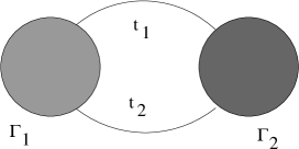
Figure 6. Joining two 1PI graphs by a pair of edges.

We can proceed similarly to give the relation between classes in the Grothendieck ring. This is in fact easier than the case of CSM classes.

Proposition 5.6.

With notation as in Corollaries 5.3 and 5.4, we have

(5.6) $$\begin{array}[]{rl}[X_{\hat{\Gamma}}]=&(1+{\mathbb{T}})\cdot[X_{\Gamma}]+[{\mathbb{P}}^{0}]\\[5.69054pt] [X_{\Gamma^{\prime}}]=&{\mathbb{T}}\cdot[X_{\Gamma}]+[{\mathbb{P}}^{n-1}]+[{\mathbb{P}}^{0}].\end{array}$$

Proof.

The class of a cone in the Grothendiek ring is just

$$[C(X)]=[(X\times{\mathbb{A}}^{1})\cup\{pt\}]=[X][{\mathbb{A}}^{1}]+[{\mathbb{A}}^{0}].$$

The result then follows immediately. ∎

As we have already noticed in our computation of the class in the Grothendieck ring and of the CSM class in the special case of the banana graphs, the formulae look nicer when written in terms of the hypersurface complement, rather than of the hypersurface itself. The same happens here. When we reformulate the above in terms of the complements of the hypersurfaces in projective space we find the following immediate consequence of additivity and of the formulae obtained previously.

Corollary 5.7.

With notation as in Corollaries 5.3 and 5.4, assume that $c({\mathbb{P}}^{n-1}\smallsetminus X_{\Gamma})=g(H)\cap[{\mathbb{P}}^{n-1}]_{*}$. Then

(5.7) $$\begin{array}[]{rl}c({\mathbb{P}}^{n}\smallsetminus X_{\hat{\Gamma}})=&(1+H)g(H)\cap[{\mathbb{P}}^{n}]_{*}\\[5.69054pt] c({\mathbb{P}}^{n}\smallsetminus X_{\Gamma^{\prime}})=&g(H)\cap[{\mathbb{P}}^{n}]_{*}\end{array}$$

Similarly, the classes in the Grothendieck group satisfy

(5.8) $$\begin{array}[]{rl}[{\mathbb{P}}^{n}\smallsetminus X_{\hat{\Gamma}}]=&(1+{\mathbb{T}})\cdot[{\mathbb{P}}^{n-1}\smallsetminus X_{\Gamma}]\\[5.69054pt] [{\mathbb{P}}^{n}\smallsetminus X_{\Gamma^{\prime}}]=&{\mathbb{T}}\cdot[{\mathbb{P}}^{n-1}\smallsetminus X_{\Gamma}].\end{array}$$

Figure 7. Graph obtained from $\Gamma_{4}$ by adding loops and subdividing edges.

We give two explicit examples obtained from the banana graphs by applying the operations discussed above.

Example 5.8.

Attach a looping edge to the banana graph $\Gamma_{4}$ of Figure 3 and then subdivide the new edge. This gives the graph in Figure 7. The CSM class of the hypersurface $X_{\Gamma_{4}}$ is

$$(3H+3H^{2}+5H^{3})\cap[{\mathbb{P}}^{3}]_{*}$$

by Theorem 4.8. According to Corollary 5.4, adding a loop gives a graph whose hypersurface has CSM class

$$((3H+3H^{2}+5H^{3})+((1+H)^{4}-H^{4})H+H^{4})\cap[{\mathbb{P}}^{4}]_{*}=(4H+7H^{2}+11H^{3}+5H^{4})\cap[{\mathbb{P}}^{4}]_{*}.$$

Subdividing the new edge (or any other edge) produces a hypersurface whose CSM class is given by

$$((1+H)(4H+7H^{2}+11H^{3}+5H^{4})+H^{5})\cap[{\mathbb{P}}^{5}]_{*}=(4H+11H^{2}+18H^{3}+16H^{4}+6H^{5})\cap[{\mathbb{P}}^{5}]_{*}.$$

This is the CSM class corresponding to the graph in the picture. In the Grothendieck group of varieties, the class of the complement of the hypersurface $X_{\Gamma_{4}}$ is

$${\mathbb{T}}^{3}+3{\mathbb{T}}^{2}+{\mathbb{T}}-1.$$

It follows immediately that the class of the complement of the hypersurface of the graph in Figure 7 is then

$${\mathbb{T}}({\mathbb{T}}+1)({\mathbb{T}}^{3}+3{\mathbb{T}}^{2}+{\mathbb{T}}-1)={\mathbb{T}}^{5}+4{\mathbb{T}}^{4}+4{\mathbb{T}}^{3}-{\mathbb{T}}.$$

Example 5.9.

Splitting one edge in a banana graph (see Figure 8) produces a particularly simple class in the Grothendieck group for the complement of the corresponding hypersurface. The class for the ‘banana split’ graph is

$${\mathbb{T}}^{n}+n{\mathbb{T}}^{n-1}+n{\mathbb{T}}^{n-2}-(-1)^{n}.$$

Figure 8. Banana split graph.

6. Banana graphs in Noncommutative QFT

Recently there has been growing interest in investigating the renormalization properties and the perturbative theory for certain quantum field theories on noncommutative spacetimes. These arise, for instance, as effective limits of string theory [16], [31]. In particular, in dimension $D=4$, when the underlying ${\mathbb{R}}^{4}$ is made noncommutative by deformation to ${\mathbb{R}}^{4}_{\theta}$ with the Moyal product, it is known that the $\phi^{4}$ theory behaves in a very interesting way. In particular, the Grosse–Wulkenhaar model was proved to be renormalizable to all orders in perturbation theory (for an overview see [21]). We do not recall here the main aspects of noncommutative field theory, as they are beyond the main purpose of this paper, but we mention the fact, which is very relevant to us, that a parametric representation for the Feynman integrals exists also in the noncommutative setting (cf. [22], [32]). When the underlying spacetime becomes noncommutative, the usual Feynman graphs are replaced by ribbon graphs, which account for the fact that, in this case, in the Feynman rules the contribution of each vertex depends on the cyclic ordering of the edges, cf. [21]. For example, in the ordinary commutative case, among the banana graphs $\Gamma_{n}$ we consider in this paper the only ones that can appear as Feynman graphs of the $\phi^{4}$ theory are the one loop case (with two external edges at each vertex), the two loop case (with one external edge at each vertex) and the three loop case as a vacuum bubble. Excluding the vacuum bubble because of the presence of the polynomial $P_{\Gamma}(t)$, we see that the effect of making the underlying spacetime noncommutative turns the remaining two graphs into the graphs of Figure 9. Notice how the two loop ribbon graph now has two distinct versions, only one of which is a planar graph. The usual Kirchhoff polynomial $\Psi_{\Gamma}(t)$ of the Feynman graph, as well as the polynomial $P_{\Gamma}(t,p)$, are replaced by new polynomials involving pairs of spanning trees, one in the graph itself and one in another associated graph which is a dual graph in the planar case and that is obtained from an embedding of the ribbon graph on a Riemann surface in the more general case. Unlike the commutative case, these polynomials are no longer homogeneous, hence the corresponding graph hypersurface only makes sense as an affine hypersurface. The relation of the hypersurface for the noncommutative case and the one of the original commutative case (also viewed as an affine hypersurface) is given by the following statement.

Proposition 6.1.

Let $\tilde{\Gamma}$ be a ribbon graph in the noncommutative $\phi^{4}$-theory that corresponds in the ordinary $\phi^{4}$-theory to a graph $\Gamma$ with $n$ internal edges. Then instead of a single graph hypersurface $X_{\Gamma}$ one has a one-parameter family of affine hypersurfaces $X_{\tilde{\Gamma},s}\subset{\mathbb{A}}^{n}$, where the parameter $s\in{\mathbb{R}}_{+}$ depends upon the deformation parameter $\theta$ of the noncommutative ${\mathbb{R}}^{4}_{\theta}$ and on the parameter $\Omega$ of the harmonic oscillator term in the Grosse–Wulkenhaar model. The hypersurface corresponding to the value $s=0$ has a singularity at the origin $0\in{\mathbb{A}}^{n}$ whose tangent cone is the (affine) graph hypersurface $X_{\Gamma}$.

Proof.

This follows directly from the relation between the graph polynomial for the ribbon graph $\tilde{\Gamma}$ given in [22] and the Kirchhoff polynomial $\Psi_{\Gamma}$. It suffices to see that (a constant multiple of) the Kirchhoff polynomial is contained in the polynomial for $\tilde{\Gamma}$ for all values of the parameter $s$, and that it gives the part of lowest order in the variables $t_{i}$ when $s=0$. ∎

In the specific examples of the banana graphs $\tilde{\Gamma}_{2}$ and $\tilde{\Gamma}_{3}$ of Figure 9, the polynomials have been computed explicitly in [22] and they are of the form

(6.1) $$\Psi_{\tilde{\Gamma}_{2}}=(1+4s^{2})(t_{1}+t_{2}+t_{1}^{2}t_{2}+t_{1}t_{2}^{2}),$$

where the parameter $s=(4\theta\Omega)^{-1}$ is a function of the deformation parameter $\theta\in{\mathbb{R}}$ of the Moyal plane and of the parameter $\Omega$ in the harmonic oscillator term in the Grosse–Wulkenhaar action functional (see [21]). One can see the polynomial $\Psi_{\Gamma_{2}}(t)=t_{1}+t_{2}$ appearing as lowest order term. Similarly for the two graphs $\tilde{\Gamma}_{3}$ that correspond to the banana graph $\Gamma_{3}$ one has ([22])

(6.2) $$\begin{array}[]{rl}\Psi_{\tilde{\Gamma}_{3}}(t)=&(1+8s^{2}+16s^{4})(t_{1}t_{2}+t_{2}t_{3}+t_{1}t_{3}+t_{1}^{2}t_{2}t_{3}+t_{1}t_{2}^{2}t_{3}+t_{1}t_{2}t_{3}^{2})\\[5.69054pt] +&16s^{2}(t_{2}^{2}+t_{1}^{2}t_{3}^{2})\end{array}$$

for the planar case, while for the non-planar case one has

(6.3) $$\begin{array}[]{rl}\Psi_{\tilde{\Gamma}_{3}}(t)=&(1+8s^{2}+16s^{4})(t_{1}t_{2}+t_{2}t_{3}+t_{1}t_{3}+t_{1}^{2}t_{2}t_{3}+t_{1}t_{2}^{2}t_{3}+t_{1}t_{2}t_{3}^{2})\\[5.69054pt] +&4s^{2}(t_{2}^{2}+t_{1}^{2}t_{3}^{2}+t_{1}^{2}+t_{2}^{2}t_{3}^{2}+t_{3}^{2}+t_{1}^{2}t_{2}^{2}+1+t_{1}^{2}t_{2}^{2}t_{3}^{2}).\end{array}$$

In both cases, one readily recognizes the polynomial $\Psi_{\Gamma_{3}}(t)=t_{1}t_{2}+t_{2}t_{3}+t_{1}t_{3}$ as the lowest order part at $s=0$. Notice how, when $s\neq 0$ one finds other terms of order less than or equal to that of the polynomial $\Psi_{\Gamma_{3}}(t)$, such as $t_{2}^{2}$ in (6.2) and $1+t_{1}^{2}+t_{2}^{2}+t_{3}^{2}$ in (6.3). Notice also how, at the limit value $s=0$ of the parameter, the two polynomials for the two different ribbon graphs corresponding to the third banana graph $\Gamma_{3}$ agree.

For each value of the parameter $s=(4\theta\Omega)^{-1}$ one obtains in this way an affine hypersurface, which is a curve in ${\mathbb{A}}^{2}$ or a surface in ${\mathbb{A}}^{3}$, and that has the corresponding affine $X_{\Gamma_{n}}$ as tangent cone at the origin in the case $s=0$. The latter is a line in the $n=2$ case and a cone on a nonsingular conic in the case $n=3$.

Figure 9. Banana graphs in noncommutative $\phi^{4}$-theory

As a further example of why it is useful to compute invariants such as the CSM classes for the graph hypersurfaces, we show that the CSM class of the hypersurface defined by the polynomial (6.2) detects the special values of the deformation parameter $s=(4\theta\Omega)^{-1}$ where the hypersurface $X_{\tilde{\Gamma}_{3}}$ becomes more singular and gives a quantitative estimate of the amount by which the singularities change.

The CSM class is naturally defined for projective varieties. In the case of an affine hypersurface defined by a non-homogeneous equation, one can choose to compactify it in projective space by adding an extra variable and making the equation homogeneous and then computing the CSM class of the corresponding projective hypersurface. However, in doing so one should be aware of the fact that the CSM class of an affine variety, defined by choosing an embedding in a larger compact ambient variety, depends on the choice of the embedding. An intrinsic definition of CSM classes for non-compact varieties which does not depend on the embedding was given in [2], [1]. However, for our purposes here it suffices to take the simpler viewpoint of making the equation homogeneous and then computing CSM classes. If we adopt this procedure, then by numerical calculations performed with the Macaulay2 program of [4] we obtain the following result.

Proposition 6.2.

Let $X_{\tilde{\Gamma}_{3}}\subset{\mathbb{P}}^{3}$ denote the affine surface defined by the equation (6.2) and let $\bar{X}_{\tilde{\Gamma}_{3}}\subset{\mathbb{P}}^{3}$ be the hypersurface obtained by making the equation (6.2) homogeneous. For general values of the parameter $s=(4\theta\Omega)^{-1}$ the CSM class is given by

(6.4) $$c(\bar{X}_{\tilde{\Gamma}_{3}})=14H^{3}+4H.$$

For the special value $s=1/2$ of the parameter, the CSM class becomes of the form

(6.5) $$c(\bar{X}_{\tilde{\Gamma}_{3}})|_{s=1/2}=5H^{3}+5H^{2}+4H,$$

while in the limit $s\to 0$ one has

(6.6) $$c(\bar{X}_{\tilde{\Gamma}_{3}})|_{s=0}=11H^{3}+4H.$$

It is also interesting to notice that, when we consider the second equation (6.3) for the non-planar ribbon graph associated to the third banana graph $\Gamma_{3}$, we see an example where the graph hypersurfaces of the non-planar graphs of noncommutative field theory no longer satisfy the positivity property of Conjecture 1.5 that appears to hold for the graph hypersurfaces of the commutative field theories. In fact, as in the case of the equation for the planar graph (6.2), we now find the following result.

Proposition 6.3.

Let $X_{\tilde{\Gamma}_{3}}\subset{\mathbb{P}}^{3}$ denote the affine surface defined by the equation (6.3) and let $\bar{X}_{\tilde{\Gamma}_{3}}\subset{\mathbb{P}}^{3}$ be the hypersurface obtained by making the equation (6.3) homogeneous. For general values of the parameter $s=(4\theta\Omega)^{-1}$ the CSM class is given by

(6.7) $$c(\bar{X}_{\tilde{\Gamma}_{3}})=33H^{3}-9H^{2}+6H.$$

The special case $s=1/2$ is given by

(6.8) $$c(\bar{X}_{\tilde{\Gamma}_{3}})|_{s=1/2}=9H^{3}-3H^{2}+6H$$

Notice that, in the case of ordinary Feynman graphs of commutative scalar field theories, all the examples where the CSM classes of the corresponding hypersurfaces have been computed explicitly (either theoretically or numerically) are planar graphs. Although it seems unlikely that planarity will play a role in the conjectured positivity of the coefficients of the CSM classes in the ordinary case, the example above showing that CSM classes of graph hypersurfaces of non-planar ribbon graphs in noncommutative field theories can have negative coefficients makes it more interesting to check the case of non-planar graphs in the ordinary case as well. It is well known that, for an ordinary graph to be non-planar, it has to contain a copy of either the complete graph $K_{5}$ on five vertices or the complete bipartite graph $K_{3,3}$ on six vertices. Either one of these graphs corresponds to a graph polynomial that is currently beyond the reach of the available Macaulay2 routine and a theoretical argument that provides a more direct approach to the computation of the corresponding CSM class does not seem to be easily available. It remains an interesting question to compute these CSM classes, especially in view of the fact that the original computations of [15] of Feynman integrals of graphs appear to indicate that the non-planarity of the graph is somehow related to the presence of more interesting periods (e.g. multiple as opposed to simple zeta values). It would be interesting to see whether it also has an effect on invariants such as the CSM class.

References

- [1] P. Aluffi, Classes de Chern des variétés singulières, revisitées. C. R. Math. Acad. Sci. Paris 342 (2006), no. 6, 405–410.
- [2] P. Aluffi, Limits of Chow groups, and a new construction of Chern-Schwartz-MacPherson classes. Pure Appl. Math. Q. 2 (2006), no. 4, 915–941.
- [3] P. Aluffi, Modification systems and integration in their Chow groups. Selecta Math. (N.S.) 11 (2005), no. 2, 155–202.
- [4] P. Aluffi, Computing characteristic classes of projective schemes. J. Symbolic Comput. 35 (2003), no. 1, 3–19.
- [5] P. Aluffi, Chern classes for singular hypersurfaces. Trans. Amer. Math. Soc. 351 (1999), no. 10, 3989–4026.
- [6] P. Aluffi, MacPherson’s and Fulton’s Chern classes of hypersurfaces, Internat. Math. Res. Notices, Vol.11 (1994) 455–465.
- [7] P. Aluffi, L.C. Mihalcea, Chern classes of Schubert cells and varieties, arXiv:math/0607752. To appear in Journal of Algebraic Geometry.
- [8] P. Belkale, P. Brosnan, Matroids, motives, and a conjecture of Kontsevich, Duke Math. Journal, Vol.116 (2003) 147–188.
- [9] J. Bjorken, S. Drell, Relativistic Quantum Mechanics, McGraw-Hill, 1964, and Relativistic Quantum Fields, McGraw-Hill, 1965.
- [10] S. Bloch, Motives associated to graphs, Japan J. Math., Vol.2 (2007) 165–196.
- [11] S. Bloch, E. Esnault, D. Kreimer, On motives associated to graph polynomials, Commun. Math. Phys., Vol.267 (2006) 181–225.
- [12] S. Bloch, D. Kreimer, Mixed Hodge structures and renormalization in physics, arXiv:0804.4399.
- [13] J.-P. Brasselet, D. Lehmann, J. Seade, T. Suwa, Milnor classes of local complete intersections, Trans. Amer. Math. Soc., Vol.354(2002) N.4, 1351–1371.
- [14] J.P. Brasselet, M.H. Schwartz, Sur les classes de Chern d’un ensemble analytique complexe, in “The Euler-Poincaré characteristic”, Astérisque, Vol.83, pp.93–147, Soc. Math. France, 1981.
- [15] D. Broadhurst, D. Kreimer, Association of multiple zeta values with positive knots via Feynman diagrams up to 9 loops, Phys. Lett. B, Vol.393 (1997) 403–412.
- [16] A.Connes, M.Douglas, A.Schwarz, Noncommutative geometry and matrix theory: compactification on tori. JHEP 9802 (1998) 3–43.
- [17] A. Connes, D. Kreimer, Renormalization in quantum field theory and the Riemann–Hilbert problem I. The Hopf algebra structure of graphs and the main theorem, Comm. Math. Phys., Vol.210 (2000) 249–273.
- [18] W. Fulton, Intersection theory. Ergebnisse der Mathematik und ihrer Grenzgebiete (3) 2. Springer-Verlag, 1984. xi+470 pp.
- [19] H. Gillet, C.Soulé, Descent, motives and -theory. J. Reine Angew. Math. 478 (1996), 127–176.
- [20] D.R. Grayson, M.E. Stillman, Macaulay 2, a software system for research in algebraic geometry, available at http://www.math.uiuc.edu/Macaulay2/
- [21] H. Grosse, R. Wulkenhaar, Renormalization of noncommutative quantum field theory, in “An invitation to Noncommutative Geometry” pp.129–168, World Scientific, 2008.
- [22] R. Gurau, V. Rivasseau, Parametric Representation of Noncommutative Field Theory, Commun. Math. Phys. Vol. 272 (2007) N.3, 811–835
- [23] C. Itzykson, J.B. Zuber, Quantum Field Theory, Dover Publications, 2006.
- [24] M. Kwieciński, Formule du produit pour les classes caractéristiques de Chern-Schwartz-MacPherson et homologie d’intersection, C. R. Acad. Sci. Paris Sér. I Math., 314(1992) N.8, 625–628.
- [25] R.D. MacPherson, Chern classes for singular algebraic varieties. Ann. of Math. (2) 100 (1974), 423–432.
- [26] M. Marcolli, Motivic renormalization and singularities, arXiv:0804.4824.
- [27] N. Nakanishi Graph Theory and Feynman Integrals. Gordon and Breach, 1971.
- [28] A. Parusiński, A generalization of the Milnor number, Math. Ann. Vol.281 (1988) N.2, 247–254.
- [29] M.H. Schwartz, Classes caractéristiques définies par une stratification d’une variété analytique complexe. I. C. R. Acad. Sci. Paris Vol.260 (1965) 3262–3264.
- [30] M.H. Schwartz, Classes caractéristiques définies par une stratification d’une variété analytique complexe, C. R. Acad. Sci. Paris, Vol.260 (1965) 3535–3537.
- [31] N. Seiberg, E. Witten, String theory and noncommutative geometry, JHEP 9909 (1999) 32–131.
- [32] A. Tanasa, Overview of the parametric representation of renormalizable non-commutative field theory, arXiv:0709.2270.