$\gamma$ measurements at LHCb

Abstract

The LHCb collaboration has studied various promising ways to determine the Unitarity Triangle angle $\gamma$. Three complementary methods will be considered. The potential of the $B\to DK^{(*)}$ decays has been studied by employing the combined Gronau-London-Wyler (GLW) and the Atwood-Dunietz-Soni (ADS) methods, making use of a large sample of simulated data. $\gamma$ can also be extracted with a time-dependent analysis of $B_{s}\to D_{s}K$ decays, provided that the $B_{s}$ mixing phase is measured independently. In addition, the combined measurement of the $B^{0}\to\pi^{+}\pi^{-}$ and $B^{0}_{s}\to K^{+}K^{-}$ time-dependent CP asymmetries allows the determination of $\gamma$, up to U-spin flavour symmetry breaking corrections. For each method the expected sensitivities to the angle $\gamma$ are presented.

I Introduction

LHCb aims to study CP violation and rare $B$-meson decays with high precision, using the Large Hadron Collider (LHC), where all species of $B$-mesons are produced in 14 $\mathrm{TeV}$ $pp$ collisions bib:lhcb1 ; bib:lhcb2 . In these events the $b\bar{b}$ pairs are frequently produced in the same forward (or backward) direction. The LHCb detector is a single-arm spectrometer with a forward coverage from 10 $\mathrm{mrad}$ to 300 $\mathrm{mrad}$ in the horizontal plane (i.e., the bending plane of the magnet). The acceptance lies between 10-250 $\mathrm{mrad}$ in the vertical plane (non-bending plane). The detector layout in the bending plane is shown in Fig. 1.

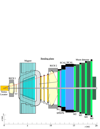
Figure 1: The LHCb setup with the different sub-detectors shown in the horizontal (bending) plane.

II Event Selection

LHCb will collect large samples of all types of $B$ mesons and baryons. These samples will allow the precise measurement of all the three ($\alpha$, $\beta$ and $\gamma$) angles of the Unitarity triangle and of the $B_{s}$ mixing phase. Here, three complementary methods to extract the Unitarity Triangle angle $\gamma$ will be considered.

As it will become clear in the next sections, the three complementary methods considered for the extraction of the Unitarity Triangle angle $\gamma$ use different techniques to determine $\gamma$. However similar approaches are used in the event selection and in the selection at the trigger level. In all cases, samples of signal and background events are simulated through the LHCb apparatus; the selection is then optimized in order to maximize the signal efficiency and minimize the background contribution. The main selection criteria used take into account that the large $B$ mass produces decay products with high $p_{T}$ and that the long $B$ lifetime produces tracks with large impact parameter with respect to the primary vertex. Furthermore particle identification cuts are used for the $\pi/K$ identification and cuts on the significance of the flight distance of the $B$ are used in order to have a $B$ detached from the primary vertex.

All the following results are for an integrated luminosity of 2 fb^-1, which corresponds to one nominal year of data taking.

III Extracting $\gamma$ from $B\to DK$ decays

Interfering tree diagrams in the $B^{\pm}\to\tilde{D}K^{\pm}$ decays allow the determination of the Unitarity Triangle angle $\gamma$. Here, $\tilde{D}$ can be a $D^{0}$ or a $\overline{D^{0}}$ and the $D^{0}$ and the $\overline{D^{0}}$ are reconstructed in a common final state.

In LHCb bib:guy this is done by employing the combined Gronau-London-Wyler (GLW) bib:glw and the Atwood-Dunietz-Soni (ADS) bib:ads methods. In the first method the information of the CP even eigenstates, where a $\tilde{D}$ decays to $\pi^{+}\pi^{-}$ or $K^{+}K^{-}$ is used. Note that reconstruction of the CP odd eigenstates, which include neutral particles, is rather challenging in LHCb and is not considered in this analysis. The ADS method exploits the interference between the favoured and double Cabibbo suppressed decay modes of the neutral D mesons to state such as $K\pi$ or $K\pi\pi\pi$. Using the ADS method the following equations can be written for the decay rates for the neutral $B^{0}\to D^{0}(\to K\pi)K^{*0}$ channels bib:kazu (very similar equation can be written for the charged decays, see also bib:patel ) :

$$\Gamma(B^{0}\to(K^{+}\pi^{-})_{D}K^{*0}) = N_{K\pi}(1+(r_{B}r_{D})^{2}+2r_{B}r_{D}\cdot$$ (1)

$$\cos(\delta_{B}+\delta_{D}+\gamma))\;\;\;,$$

$$\Gamma(B^{0}\to(K^{-}\pi^{+})_{D}K^{*0}) = N_{K\pi}(r_{B}^{2}+r_{D}^{2}+2r_{B}r_{D}\cdot$$ (2)

$$\cos(\delta_{B}-\delta_{D}+\gamma))\;\;\;,$$

$$\Gamma(\overline{B^{0}}\to(K^{-}\pi^{+})_{D}\overline{K^{*0}}) = N_{K\pi}(1+(r_{B}r_{D})^{2}+2r_{B}r_{D}\cdot$$ (3)

$$\cos(\delta_{B}+\delta_{D}-\gamma))\;\;\;,$$

$$\Gamma(\overline{B^{0}}\to(K^{+}\pi^{-})_{D}\overline{K^{*0}}) = N_{K\pi}(r_{B}^{2}+r_{D}^{2}+2r_{B}r_{D}\cdot$$ (4)

$$cos(\delta_{B}-\delta_{D}-\gamma))\;\;\;,$$

where

$$r_{B}=\frac{|A(B^{0}\to D^{0}K^{*0})|}{|A(B^{0}\to\overline{D^{0}}K^{*0})|}$$

is the ratio of the magnitudes between the two amplitudes of the B-decay and similarly

$$r_{D}=\frac{|A(D^{0}\to K^{+}\pi^{-})|}{|A(\overline{D^{0}}\to K^{+}\pi^{-})|}\;\;\;.$$

Furthermore $\delta_{B}$ represents the strong phase difference between the two B-decays while $\delta_{D}$ represents the strong phase difference between the two D-decays. $N_{K\pi}$ gives the overall normalization and represents the total number of $B^{0}\to(K\pi)_{D}K^{*0}$ events. It can be seen that there are two favoured rates (1) and (3) and two suppressed rates (2) and (4). Further information can be added by including the decays to CP-eigenstates, such as $\pi^{+}\pi^{-}$ or $K^{+}K^{-}$ and so:

$$\Gamma(B^{0}\to D_{CP}K^{*0}) = N_{CP}(1+r_{B}^{2}+$$ (5)

$$2r_{B}\cos(\delta_{B}+\gamma))\;\;\;,$$

$$\Gamma(\overline{B^{0}}\to D_{CP}\overline{K^{*0}}) = N_{CP}(1+r_{B}^{2}+$$ (6)

$$2r_{B}\cos(\delta_{B}-\gamma))\;\;\;.$$

Here, $N_{CP}$ represents the total number of $B^{0}\to D_{CP}K^{*0}$ events. Note that $r_{D}$ is known and is equal to 0.060 $\pm$ 0.003 bib:pdg and $N_{CP}$ can be calculated from $N_{K\pi}$ taking into account the different efficiencies and branching ratios. Furthermore, for what concerns $r_{B}$, for the neutral $B$, values smaller than 0.6 with 95% probability have been measured at Babar bib:babarneutro , while for the charged $B$ the latest world average value is $r_{B}=0.10\pm 0.02$ bib:ut . $\delta_{B}$ is unknown for the neutral $B$-meson, while its value is fixed at 130^∘ for the charged $B$-meson bib:babar ; bib:belle . $\delta_{D}$ is assumed to be in the range [-25^∘; +25^∘] due to a limit set by the CLEO-c collaboration bib:cleoc . In total there are 5 unknowns ($\gamma$, $r_{B}$, $\delta_{B}$, $\delta_{D}$ and $N_{K\pi}$) and 6 observables.

III.1 Sensitivity to $\gamma$

As a result of the event selection, the annual yields together with the total efficiencies and with the background to signal ratios are listed in Table 1  bib:kazu ; bib:patel .

Channel	$\epsilon_{tot}$ [%]	S	$B_{b\bar{b}}/S$
$B^{0}\to\overline{D^{0}}(K^{+}\pi^{-})K^{*0}$	0.33	3350	$<$ 2.0
$B^{0}\to D^{0}(K^{+}\pi^{-})K^{*0}$	0.33	536	$<$ 12.8
$B^{0}\to D_{CP}(K^{+}K^{-})K^{*0}$	0.46	474	$<$ 4.1
$B^{0}\to D_{CP}(\pi^{+}\pi^{-})K^{*0}$	0.36	134	$<$ 14
$B^{+}\to\overline{D^{0}}(K^{+}\pi^{-})K^{+}$	0.50	28000	0.63
$B^{+}\to\overline{D^{0}}(K^{-}\pi^{+})K^{+}$	0.50	100	7.8
$B^{+}\to\overline{D^{0}}(K^{+}K^{-})K^{+}$	0.51	3000	1.2
$B^{+}\to\overline{D^{0}}(\pi^{+}\pi^{-})K^{+}$	0.58	1000	3.6

Table 1: Summary of event yield ($S$), experimental efficiency ($\epsilon_{tot}$), and background to signal ratios.

Both for the charged and neutral $B$-meson decays a standalone Monte Carlo (MC) simulation was used to generate the event yields and fit the unknown parameters. All the unknown parameters have been scanned as shown in Table 2. The input value of $\gamma$ has been fixed at 60^∘.

Parameter	Scan range
	$B^{0}\to D^{0}K^{*0}$	$B^{\pm}\to D^{0}K^{\pm}$
$\delta_{B}$	[-180∘ ; +180∘]	fixed at 130∘
$\delta_{D}$	[-25∘ ; +25∘]	[-25∘ ; +25∘]
$r_{B}$	[0.0 ; 0.6]	[0.0 ; 0.2]

Table 2: Scan ranges of the input parameters of the toy used for the extraction of $\gamma$ for both the charged and the neutral $B$-mesons. Note that while $\delta_{B}$ has been scanned in the full range for the neutral $B$-meson, its value was fixed at 130^∘ for the charged $B$-meson bib:babar ; bib:belle . $\delta_{D}$ has been scanned in the range [-25^∘; +25^∘] due to a limit set by the CLEO-c collaboration bib:cleoc . For what concerns $r_{B}$, for the neutral $B$, values smaller than 0.6 with 95% probability have been measured at Babar bib:babarneutro , while for the charged $B$ the latest world average value is $r_{B}=0.10\pm 0.02$ bib:ut .

For the charged $B$-meson with one year of data at nominal luminosity (2fb^-1), the angle $\gamma$ can be determined with a precision in the range $8.2^{\circ}-9.6^{\circ}$, depending on the value of the strong phase $\delta_{D}$ bib:patel . For the neutral $B$ the angle $\gamma$ can be determined with a precision smaller than $10^{\circ}$, depending on the value of the strong phase $\delta_{B}$ and for $r_{B}$ values bigger than 0.3 bib:kazu .

IV Extracting $\gamma$ from $B^{0}_{s}\to D_{s}K$ decays

The relations between the $B^{0}$-meson mass eigenstates $|B_{H,L}\rangle$ and their flavour eigenstates $|B^{0}\rangle$ and $\overline{|B^{0}}\rangle$, can be expressed in terms of linear coefficients $p$ and $q$:

$$|B_{H,L}\rangle=p|B^{0}\rangle\mp q\overline{|B^{0}}\rangle\;\;\;.$$ (7)

The difference in mass and decay rates are defined as:

$$\Delta m=m_{H}-m_{L}\;\;\;\;,\;\;\;\Delta\Gamma=\Gamma_{H}-\Gamma_{L}\;\;\;.$$ (8)

The average mass and decay rate are defined as:

$$m=\frac{m_{H}+m_{L}}{2}\;\;\;\;,\;\;\;\Gamma=\frac{\Gamma_{H}+\Gamma_{L}}{2}\;\;\;.$$ (9)

The decay rate at a time $t$ of an originally produced $|B^{0}\rangle$ to a final state $f$ is given by:

$$\Gamma_{B^{0}\to f}(t)=|\langle f|T|B^{0}(t)\rangle|^{2}\;\;\;,$$ (10)

where T is the transition matrix element. The time evolution of the flavour eigenstates $|B^{0}\rangle$ and $|\overline{B^{0}}\rangle$ is then given by the four decay equations:

$$\Gamma_{B\to f}(t) = \left|A_{f}\right|^{2}(1+|\lambda_{f}|^{2})\frac{e^{-\Gamma t}}{2}\cdot$$

$$(\cosh{\frac{\Delta\Gamma t}{2}}+D_{f}\sinh{\frac{\Delta\Gamma t}{2}}+$$

$$C_{f}\cos{\Delta mt}-S_{f}\sin{\Delta mt})\;\;\;,$$

$$\Gamma_{\overline{B}\to f}(t) = \left|A_{f}\right|^{2}\left|\frac{p}{q}\right|^{2}(1+|\lambda_{f}|^{2})\frac{e^{-\Gamma t}}{2}\cdot$$

$$(\cosh{\frac{\Delta\Gamma t}{2}}+D_{f}\sinh{\frac{\Delta\Gamma t}{2}}$$

$$-C_{f}\cos{\Delta mt}+S_{f}\sin{\Delta mt})\;\;\;,$$

$$\Gamma_{\overline{B}\to\overline{f}}(t) = \left|\overline{A}_{\overline{f}}\right|^{2}(1+|\overline{\lambda}_{\overline{f}}|^{2})\frac{e^{-\Gamma t}}{2}\cdot$$

$$(\cosh{\frac{\Delta\Gamma t}{2}}+D_{\overline{f}}\sinh{\frac{\Delta\Gamma t}{2}}$$

$$+C_{\overline{f}}\cos{\Delta mt}-S_{\overline{f}}\sin{\Delta mt})\;\;\;,$$

$$\Gamma_{B\to\overline{f}}(t) = \left|\overline{A}_{\overline{f}}\right|^{2}\left|\frac{p}{q}\right|^{2}(1+|\overline{\lambda}_{\overline{f}}|^{2})\frac{e^{-\Gamma t}}{2}\cdot$$

$$(\cosh{\frac{\Delta\Gamma t}{2}}+D_{\overline{f}}\sinh{\frac{\Delta\Gamma t}{2}}$$

$$-C_{\overline{f}}\cos{\Delta mt}+S_{\overline{f}}\sin{\Delta mt})\;\;\;,$$

where

$$D_{f} = \frac{2Re{\lambda_{f}}}{1+|\lambda_{f}|^{2}}\;\;\;,$$

$$C_{f} = \frac{1-|\lambda_{f}|^{2}}{1+|\lambda_{f}|^{2}}\;\;\;,$$

$$S_{f} = \frac{2Im{\lambda_{f}}}{1+|\lambda_{f}|^{2}}\;\;\;.$$ (12)

$A_{f}$ and $\overline{A}_{\overline{f}}$ are the decay amplitudes (e.g. $A_{f}=\langle f|T|B^{0}\rangle$) and

$$\lambda_{f}=\frac{q}{p}\frac{\overline{A}_{f}}{A_{f}}\;\;\;,\;\;\;\lambda_{\overline{f}}=\frac{q}{p}\frac{\overline{A}_{\overline{f}}}{A_{\overline{f}}}\;\;\;.$$ (13)

For the $B_{s}^{0}\to D_{s}^{\mp}K^{\pm}$ decay channels (see Feynman diagrams in Fig. 2) a $B^{0}_{s}$, as well as a $\overline{B^{0}_{s}}$, can decay directly to $D_{s}^{-}K^{+}$ or $D_{s}^{+}K^{-}$.

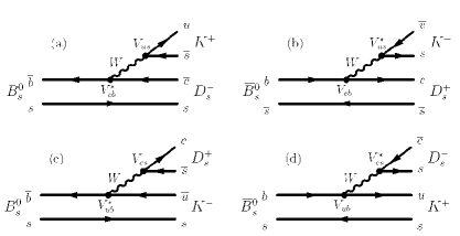
Figure 2: Feynman diagrams for the $B_{s}^{0}\to D_{s}^{-}K^{+}$ (a), $\overline{B_{s}^{0}}\to D_{s}^{+}K^{-}$ (b), $B_{s}^{0}\to D_{s}^{+}K^{-}$ (c), $\overline{B_{s}^{0}}\to D_{s}^{-}K^{+}$ (d) decays.

In addition, these relations hold for the decay amplitudes: $|A_{f}|=|\overline{A}_{\overline{f}}|$ and $|A_{\overline{f}}|=|\overline{A}_{f}|$. Assuming $|\frac{q}{p}|=1$, it is possible to write $|\lambda_{f}|=|\overline{\lambda}_{\overline{f}}|$. The terms $\lambda_{f}$ and $\overline{\lambda}_{\overline{f}}$ are calculated as

$$\lambda_{D^{-}_{s}K^{+}} = \left(\frac{q}{p}\right)_{B_{s}}\frac{\overline{A}_{D^{-}_{s}K^{+}}}{A_{D^{-}_{s}K^{+}}}=\left(\frac{V_{tb}^{*}V_{ts}}{V_{tb}V_{ts}^{*}}\right)\left(\frac{V_{ub}V_{cs}^{*}}{V_{cb}^{*}V_{us}}\right)\cdot$$

$$\left|\frac{A_{2}}{A_{1}}\right|e^{i\Delta_{s}}=|\lambda_{D^{-}_{s}K^{+}}|e^{i(\Delta_{s}-(\gamma+\phi_{s}))}\;,$$

$$\overline{\lambda}_{D^{+}_{s}K^{-}} = \left(\frac{p}{q}\right)_{B_{s}}\frac{A_{D^{+}_{s}K^{-}}}{\overline{A}_{D^{+}_{s}K^{-}}}=\left(\frac{V_{tb}V_{ts}^{*}}{V_{tb}^{*}V_{ts}}\right)\left(\frac{V_{ub}^{*}V_{cs}}{V_{cb}V_{us}^{*}}\right)\cdot$$

$$\left|\frac{A_{2}}{A_{1}}\right|e^{i\Delta_{s}}=|\lambda_{D^{-}_{s}K^{+}}|e^{i(\Delta_{s}+\gamma+\phi_{s})}\;,$$

where $|A_{2}/A_{1}|$ is the ratio of the hadronic amplitudes, which is expected to be of order unity, $\Delta_{s}$ is the strong phase difference between $A_{1}$ and $A_{2}$ and $\gamma+\phi_{s}$ is the weak phase. The $\phi_{s}$ angle originates from $B^{0}_{s}$ mixing and can be measured directly using the $B_{s}^{0}\to J/\psi\phi$ decay bib:lfernandez .

IV.1 Sensitivity to $\gamma+\phi_{s}$

As a result of the event selection, the annual yields together with the total efficiencies and with the background to signal ratios are listed in Table 3.

	S	$\epsilon_{tot}$ [%]	$B_{b\bar{b}}/S$
$B_{s}^{0}\to D_{s}^{\mp}K^{\pm}$	6200	0.32	$<$ 0.7

Table 3: Summary of event yield ($S$), experimental efficiency ($\epsilon_{tot}$), and background to signal ratios.

In a toy MC study multidimensional probability functions (PDFs) are constructed. These are supposed to mimic the outcome of an analysis of data acquired at LHCb. So first the behaviour of the experiment is described building different PDFs. In the toy in use for the sensitivity studies of the $B^{0}_{s}\to D_{s}K$ channels several PDFs describing the mass distribution, the proper time acceptance, the flavour tagging and the particle identification response have been built both for the signal events and for the background events according to the studies done with the full Geant 4 simulation bib:geant . The final PDF is built as the product of all the different PDFs and finally a likelihood fit to the generated data is performed to extract the parameters and their errors. In this toy not only the $B^{0}_{s}\to D_{s}K$ decay channels are considered, but also the topologically similar $B^{0}_{s}\to D_{s}\pi$ decay channels. The $B^{0}_{s}\to D_{s}\pi$ decay channel has a larger branching ratio and consequently a higher annual yield (140000 events) and it allows for the determination of the $\Delta m_{s}$ parameter. A summary of the input parameters that are used is given in Tab. 4.

Parameter	Input value
$\sigma(m_{B^{0}_{s}})$ (MeV)	14
$\Delta\Gamma_{s}/\Gamma_{s}$	0.1
$\Delta m_{s}(ps^{-1})$	17.5
mistag fraction $\omega$	0.328
tagging efficiency $\epsilon_{tag}$	0.5812
$|\lambda_{f}|$	0.37
$\gamma+\phi_{s}$ (∘)	60
$\Delta_{T1/T2}$ (∘)	0
$B^{0}_{s}\to D_{s}^{-}\pi^{+}$ annual yield	140k
$B^{0}_{s}\to D_{s}^{\mp}K^{\pm}$ annual yield	6.2k
$B^{0}_{s}\to D_{s}^{-}\pi^{+}$ B/S ratio	0.2
$B^{0}_{s}\to D_{s}^{\mp}K^{\pm}$ B/S ratio	0.7

Table 4: Input parameter values for the toy MC simulation program.

The final sensitivity results are shown in Tab. 5. It can be seen that with one year of data taking at nominal luminosity a sensitivity on $\gamma+\phi_{s}$ of 10.3^∘ can be obtained. A more detailed study can be found in bib:scohen .

	$\Delta m_{s}(ps^{-1})$	$|\lambda_{f}|$	$\Delta_{T1/T2}$ (∘)	$\gamma+\phi_{s}$ (∘)
Input value	17.5	0.37	0	60
Fitted value	17.5	0.372	0	60.4
$\sigma$ (1y)	0.007	0.061	10.3	10.3
$\sigma$ (5y)	0.003	0.027	4.6	4.6

Table 5: Summary of the sensitivity results for the toy for $B^{0}_{s}\to D_{s}^{\mp}K^{\pm}$ and $B^{0}_{s}\to D_{s}^{-}\pi^{+}$ events.

V Extracting $\gamma$ from $B^{0}\to\pi^{+}\pi^{-}$ and $B^{0}_{s}\to K^{+}K^{-}$

In this section the way to extract $\gamma$ through the combined measurement of the $B^{0}\to\pi^{+}\pi^{-}$ and $B^{0}_{s}\to K^{+}K^{-}$ CP asymmetries and under the assumption of invariance of the strong interaction under the $d$ and $s$ quarks exchange (U-spin symmetry) bib:fleis is described. In Fig. 3 the $B_{(s)}^{0}\to h^{+}h^{\prime-}$ tree diagrams are shown.

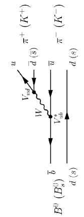
Figure 3: The $B_{(s)}^{0}\to h^{+}h^{\prime-}$ tree diagram.

For a neutral $B$-meson decaying into a CP eigenstate $f$, the time-dependent CP asymmetry is given by:

$${\cal A}_{CP}(t) = \frac{\Gamma(\overline{B^{0}}_{d/s}(t)\to f)-\Gamma(B^{0}_{d/s}(t)\to f)}{\Gamma(\overline{B^{0}}_{d/s}(t)\to f)+\Gamma(B^{0}_{d/s}(t)\to f)}$$ (15)

$$= \frac{-C_{CP}\cos\Delta mt+S_{CP}\sin\Delta mt}{\cosh\frac{\Delta\Gamma}{2}t-A_{CP}^{\Delta\Gamma}\sinh\frac{\Delta\Gamma}{2}t},$$

where $\Gamma(\overline{B^{0}}_{d/s}(t)\to f)$ and $\Gamma(B^{0}_{d/s}(t)\to f)$ are the decay rates of the initial $\overline{B}$ and $B$ states respectively, and $\Delta m$ and $\Delta\Gamma$ are the mass and width differences between the two mass eigenstates.

As shown in bib:fleis $C_{CP}$ and $S_{CP}$ for the $B^{0}\to\pi^{+}\pi^{-}$ and $B^{0}_{s}\to K^{+}K^{-}$ can be written as functions of the Unitarity Triangle angle $\gamma$, and of the two hadronic parameters $d$ and $\theta$ (which parametrize respectively the magnitude and phase of the penguin-to-tree amplitude ratio), as follows

$$C_{\pi\pi} = \frac{2d\sin\theta\sin\gamma}{1-2d\cos\theta\cos\gamma+d^{2}}\;\;,$$

$$S_{\pi\pi} = \frac{\sin{(\phi_{d}+2\gamma})-2d\cos{\theta}\sin{(\phi_{d}+\gamma})+d^{2}\sin{\phi_{d}}}{1-2d\cos{\theta}\cos{\gamma}+d^{2}}\;\;,$$

$$C_{KK} = -\frac{2d^{\prime}\sin{\theta^{\prime}}\sin{\gamma}}{1+2d^{\prime}\cos{\theta^{\prime}}\cos{\gamma}+d^{\prime 2}}\;\;,$$

$$S_{KK} = \frac{\sin{(\phi_{s}+2\gamma})+2d^{\prime}\cos{\theta^{\prime}}\sin{(\phi_{s}+\gamma})+d^{\prime 2}\sin{\phi_{s}}}{1+2d^{\prime}\cos{\theta^{\prime}}\cos{\gamma}+d^{\prime 2}}\;\;,$$

where $\phi_{d}$ and $\phi_{s}$ are the $B^{0}_{d}/\overline{B^{0}_{d}}$ and $B^{0}_{s}/\overline{B^{0}_{s}}$ mixing phases which in LHCb will be measured from $B_{d}^{0}\to J/\psi K_{S}$ decay and from $B_{s}^{0}\to J/\psi\phi$ respectively bib:lfernandez . This system of four equations and five unknowns ($d,d^{\prime},\theta,\theta^{\prime}$ and $\gamma$) can be solved with the help of the U-spin symmetry, as a consequence $d=d^{\prime}$ and $\theta=\theta^{\prime}$. This results in an over-constrained system of three unknowns and four equations.

V.1 Sensitivity to the CP asymmetries and to $\gamma$

As a result of the event selection, the annual yields together with the total efficiencies and with the background to signal ratios are listed in Table 6.

Event type	$BR$	S	$\epsilon_{tot}$ [%]	$B_{b\bar{b}}/S$	$B_{sp}/S$
	($\times 10^{-6}$)
$B^{0}_{d}\to\pi^{+}\pi^{-}$	4.8	35700	0.93	0.46	0.08
$B^{0}_{d}\to K^{+}\pi^{-}$	18.5	137600	0.93	0.14	0.02
$B^{0}_{s}\to\pi^{+}K^{-}$	4.8	9800	1.02	1.92	0.54
$B^{0}_{s}\to K^{+}K^{-}$	18.5	35900	0.97	$<$ 0.06	0.06

Table 6: Summary of event yields ($S$), Branching ratios, experimental efficiency ($\epsilon_{tot}$), and background to signal ratios, considering both the $b\bar{b}$ combinatorial background and the specific background.

As for the $B^{0}_{s}\to D_{s}K$ decays a toy MC is used to mimic the outcome of an analysis of data acquired at LHCb. In this toy, used for the CP sensitivity studies of the $B_{(s)}^{0}\to h^{+}h^{\prime-}$ channels, several PDFs describing the mass distribution, the proper time acceptance, the flavour tagging and the particle ID response have been built both for the signal events and for the background events according to the studies done with the full Geant 4 simulation bib:sens . The final PDF is built as the product of all the different PDFs and a likelihood fit to the generated data is performed to extract the parameters and their errors.

The extraction of $\gamma$ is then performed using a Bayesian approach in three different U-spin scenarios:

• Assuming perfect U-spin symmetry: $d=d^{\prime}$ and $\theta=\theta^{\prime}$ .

• With a weaker assumption on the U-spin symmetry: $d=d^{\prime}$ and no constraint on $\theta$ and $\theta^{\prime}$.

• With an even weaker assumption on the U-spin symmetry: $\xi=d^{\prime}/d=$ [0.8,1.2] and no constraint on $\theta$ and $\theta^{\prime}$.

In the three different cases the sensitivity on $\gamma$ is taken considering the 68% probability interval of the resulting PDF distribution for $\gamma$.

Fig. 4 shows an example of a resulting PDF for $\gamma$ obtained assuming perfect U-spin symmetry. The 68% and 95% probability intervals are visible. The 68% probability interval corresponds to a sensitivity of 4^∘. The sensitivity in the second and in the third scenarios increases and varies between 7^∘ and 10^∘.

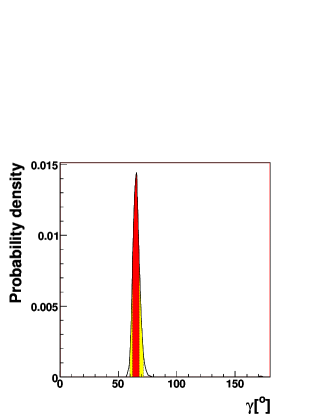
Figure 4: $\gamma$ probability density obtained in case of perfect U-spin symmetry. The 68% and 95% probability intervals are visible. The 68% probability interval corresponds to a sensitivity of 4^∘. The plot has been obtained using tools developed by the UTfit Collaboration bib:utfit .

It is important to note that the extraction of $\gamma$ by means of the $B^{0}\to\pi^{+}\pi^{-}$ and $B^{0}_{s}\to K^{+}K^{-}$ decays uses not only tree diagrams but also loop diagrams and is therefore sensitive to new physics.

VI Conclusions

In these proceedings three complementary methods for the extraction of the Unitarity Triangle angle $\gamma$ have been discussed.

The potential of the $B\to DK^{(*)}$ decays has been studied by employing the combined Gronau-London-Wyler (GLW) and the Atwood-Dunietz-Soni (ADS) methods. For the charged $B$-meson, with one year of data at nominal luminosity, the angle $\gamma$ can be determined with a precision in the range $8^{\circ}-10^{\circ}$, depending on the value of the strong phase $\delta_{D}$ bib:patel . For the neutral $B$, the angle $\gamma$ can be determined with a precision smaller than $10^{\circ}$, depending on the value of the strong phase $\delta_{B}$ and for $r_{B}$ values bigger than 0.3 bib:kazu .

It has been shown that the angle $\gamma$ can also be extracted with a time-dependent analysis through the $B_{s}\to D_{s}K$ decays, provided that the $B_{s}$ mixing phase is measured independently. With one year of data taking at nominal luminosity, a sensitivity on $\gamma+\phi_{s}$ of 10^∘ can be obtained.

The combined measurement of the $B^{0}\to\pi^{+}\pi^{-}$ and $B^{0}_{s}\to K^{+}K^{-}$ time-dependent CP asymmetries allows the determination of the Unitarity Triangle angle $\gamma$, up to U-spin flavour symmetry breaking corrections. Here a sensitivity of 10^∘, with one year of data taking at nominal luminosity, can also be obtained, but the final results depend on the assumption on the breaking of the U-spin symmetry. This method uses not only tree diagrams but also loop diagrams and is therefore sensitive to new physics.

Other methods, including $B\to D(KK\pi\pi)K$ and $B\to D(K_{s}\pi^{+}\pi^{-})K$ decays, to extract $\gamma$ at LHCb have been studied. More details can be found in bib:15 ; bib:13 .

References

- (1) LHCb Collaboration, LHCb Technical Proposal, CERN-LHCC/1998-004.
- (2) LHCb Collaboration, LHCb Technical Design Report, CERN-LHCC/2003-030.
- (3) G. Wilkinson, CERN-LHCb/2005-066.
-
(4)
M. Gronau and D. London, Phys. Lett. B253,(1991) 483.
M. Gronau and D. Wyler, Phys. Lett. B265, (1991) 172. - (5) M. Atwood, I. Dunietz and A. Soni, Phys. Rev. Lett. 78 (1997) 3257.
- (6) K. Akiba et al., CERN-LHCb/2007-050.
-
(7)
M. Patel, CERN-LHCb/2006-066.
M. Patel, CERN-LHCb/2008-011. - (8) Particle Data Group, S. Eidelman et al., Phys. Lett. B592 (2004) 677.
- (9) Babar Collaboration, ArXiv 0805.2001.
- (10) V. Sordini(results obtained by the UTFit collaboration), The CKM angle - B-factories results review, Rencontres de Moriond Electroweak, 2008.
- (11) Babar Collaboration, hep-ex/0607104.
- (12) A. Poluetkov et al., Belle Collaboration, Phys. Rev. D70, 072003 (2004).
- (13) J. Rosner et al., Phys. Rev. Lett. 100, 221801 (2008).
- (14) L. Fernandez, CERN-LHCb/2006-047.
- (15) See http://www-spires.dur.ac.uk/cgi-bin/spiface/hep/www?j=NUIMA,A506,250.
- (16) S. Cohen et al., CERN-LHCb/2007-041.
- (17) R. Fleisher, Phys Rev. Lett. B 459, 306 (1999).
- (18) A. Carbone et al., CERN-LHCb/2007-059.
- (19) See http://www.utfit.org
- (20) J. Libby, CERN-LHCb 2007-141.
- (21) J. Libby et al., CERN-LHCb 2007-098.