Quantum Cloning without Interference

Abstract

We study the role of interference in the process of quantum cloning. We show that in order to achieve better than classical cloning of a qubit no interference is needed. In particular, a large class of symmetric universal 1$\to$ 2 qubit cloners exists which achieve the optimal average fidelity $5/6$ for such machines, without using any interference. We also obtain optimal average fidelities for interference–free cloning in asymmetric situations, and discuss the relation of the quantum cloners found to the Bužek–Hillery quantum cloner.

I Introduction

The celebrated no-cloning theorem Wootters and Zurek (1982) states that unknown quantum states cannot be perfectly copied, i.e. no quantum mechanical evolution exists which would transform a quantum state $\psi$ according to $\psi\rightarrow\psi\otimes\psi$ for any unknown $\psi$. This theorem is at the basis of the security of quantum key distribution systems, and has thus tremendous technological implications. From the theoretical point of view, it is a simple consequence of the linearity of quantum mechanical time evolution. A corresponding theorem for classical probability distributions can be proved just as easily: Propagating classical probability distributions linearly (e.g. phase space densities according to the Liouville equation) does not allow to transform any unknown probability distribution $p$ according to $p\rightarrow p\otimes p$. So how could you download a perfect copy of this article?

Classical and quantum information differ fundamentally by the fact that for classical systems we have (at least in principle) unrestricted access to the distributed quantities themselves (e.g. positions and momenta of particles in phase space), whereas for quantum systems we do not. In every–day language, we understand under classical copying measuring those quantities, and then preparing another system with the same values of those quantities. Indeed, a photocopy machine measures the position of bits of ink on the page, assumes that their momenta are zero (but could in principle also measure them), and then prepares an arbitrarily large number of other pages with the same positions of bits of inks with zero momentum. If we work with an ensemble of initial documents, differing slightly in the positions of bits of ink, such that it is worth talking about a probability distribution $p$, the latter will obviously be copied perfectly by the copy machine as well if it copies each member of the ensemble perfectly — but the transformation is manifestly non–linear.

According to quantum mechanics, all information about a quantum system is encoded in the wavefunction $\psi$, and $\psi$ never attributes a sharp value to both positions and momenta of the particles involved. More importantly, the apparent failure of “local hidden variable” descriptions of quantum mechanical correlations confronted with experiments testing Bell-type inequalities Aspect et al. (1982); Weihs et al. (1998); Aspect (1999); Rowe et al. (2001) suggests that in a quantum mechanical system physical observables do not even have an objective value till the observable is measured. Quantum cloning aims therefore directly at reproducing the wavefunction rather than, say, the coordinates and momenta of individual particles. If we want to compare classical and quantum copying on equal footing, we should consider directly linear transformations (stochastic maps) of the initial probability distributions in the classical case, and this is what we are going to do below.

Shortly after the publication of the no–cloning theorem, Bužek and Hillery (BH) showed that pretty good approximate cloning is possible Bužek and Hillery (1996). They invented a 1 $\rightarrow$ 2 quantum copying machine which takes a first qubit $A$ in an unknown pure state $|\psi\rangle=\alpha|0\rangle+\beta|1\rangle$ and a second qubit $B$ in a fixed known initial pure state $|0\rangle$ (an “empty page”) as input and produces two mixed states $\rho_{A}^{\prime}=\rho_{B}^{\prime}=\frac{5}{6}|\psi\rangle\langle\psi|+\frac{1}{6}|\psi^{\perp}\rangle\langle\psi^{\perp}|$, where $|\psi^{\perp}\rangle=\alpha^{*}|1\rangle-\beta^{*}|0\rangle$ is the state orthogonal to $|\psi\rangle$. A single ancilla qubit is necessary to perform the transformation. The BH machine is manifestly symmetric, i.e. the fidelities $F_{j}$ obtained as overlap of the final mixed states with the initial pure state of $A$, $F_{j}=\langle\psi|\rho_{j}^{\prime}|\psi\rangle$, $j=A,B$, are the same. It is also universal, in the sense that it copies all initial states $|\psi\rangle$ with the same fidelity $F_{j}=5/6$. Later it was shown that $5/6$ is indeed the optimal fidelity for symmetric universal $1\rightarrow 2$ cloners of a qubit Gisin and Massar (1997); Bruß et al. (1998), and that this is the largest fidelity compatible with the non–signaling constraint imposed by special relativity Gisin (1998).

For non–universal cloners, the fidelities $F_{j}(\theta,\phi)=\langle\psi(\theta,\phi)|\rho_{j}^{\prime}|\psi(\theta,\phi)\rangle$ depend on the initial states $|\psi(\theta,\phi)\rangle$, parametrized by polar and azimuthal angles $\theta$ and $\phi$ on the Bloch sphere. It is then convenient to introduce average fidelities $\overline{F}_{A}=\overline{F}_{B}$,

$$\overline{F}_{j}=\frac{1}{4\pi}\int_{0}^{2\pi}d\phi\int_{0}^{\pi}d\theta\,F_{j}(\theta,\phi)\sin\theta\,.$$ (1)

The best possible classical cloning of a qubit with symmetric average fidelities leads to $\overline{F}_{A}=\overline{F}_{B}=2/3$ Horodecki et al. (1999). The cloning is classical in the sense introduced above, i.e. the cloner acts with a classical stochastic map on the vector of probabilities corresponding to the initial state, while it has no access to the quantum coherences. We will provide a new and simple demonstration of this result below. The optimal classical fidelities are very easily matched by quantum cloning. A universal symmetric quantum cloner with fidelities $\overline{F}_{A}=\overline{F}_{B}=2/3$ can be constructed trivially by measuring the first qubit in an orthogonal basis chosen randomly and uniformly over the Bloch sphere, and preparing the second qubit in the state found in the measurement Scarani et al. (2005). Another trivial symmetric universal cloning machine leaves the original qubit unperturbed, produces the new one in a random pure state, and swaps the two with probability 1/2. It has fidelities $\overline{F}_{A}=\overline{F}_{B}=3/4$.

As always, when a quantum protocol offers a higher performance than the best possible classical scenario, it is natural to ask which quantum resource is at the origin of this difference. “Entanglement” and “Interference” are two obvious candidates Bennett and DiVincenzo (2000). In Scarani et al. (2005) it was argued that quantum cloners without coherent interaction between original qubit and copy should have fidelities limited by the one obtainable from the second “trivial” cloning strategy described above. Bruß and Macchiavello studied the entanglement at the output of a universal quantum cloner (QC) and found that bipartite entanglement between two outputs vanishes for $N\to M$ quantum cloners ($N$ identical input qubits, $M$ output qubits) in the “classical” limit $M\to\infty$ ($N$ fixed) of infinitely many copies, and in fact as soon as $M\geq N+2$. Bruß and Macchiavello (2003). The fact that classical cloning discards the quantum coherences whereas quantum cloning need not, leads naturally to the hypothesis that interference should play an important role in quantum cloning. Put the other way round, it seems likely that a cloner which uses no interference at all should not be able to outperform classical cloning. Surprisingly, we show in this article that the contrary is true: A large continuous class of quantum cloners exists which use strictly zero interference, but which outperform classical cloning, and in fact give the maximal possible average fidelity $5/6$ in the symmetric case.

Evidently, in order to study this question, the concept of interference needs to be made precise. A quantitative measure of interference was introduced in Braun and Georgeot (2006), and was used to study interference in quantum algorithms. This led to the hypothesis that an exponential amount of interference is needed in any unitary quantum algorithm which offers an exponential speed up over the corresponding classical algorithm. The hypothesis was supported by further numerical evidence in a study of disturbed versions of Grover’s and Shor’s algorithms Braun and Georgeot (2008). In Arnaud and Braun (2007) we demonstrated that the interference in a randomly chosen quantum algorithm is with high probability close to the maximum possible value, whereas in Lyakhov et al. (2007) we showed that interference plays at most a minor role in the transfer of quantum information through spin chains.

Below we briefly review the interference measure. We will then formulate quantum cloners very generally in terms of a dynamical matrix Życzkowski and Bengtsson (2004), and rewrite the interference measure using the dynamical matrix. The average fidelities are linear functions in the matrix elements, and it turns out that vanishing interference leads to linear constraints. Finding the optimal average fidelity becomes an instance of semi-definite programming, which we solve both for given $\overline{F}_{A}$ or $\overline{F}_{B}$, and for $\overline{F}_{A}=\overline{F}_{B}$. The latter case leads to one specific quantum cloner, very similar to the BH quantum cloner, and in particular with the same optimal average fidelities. We show, however, that starting from that machine a whole continuous class of other machines can be constructed with the same optimal average fidelities and vanishing interference.

A final remark is in order concerning the applicability of our results to quantum broadcasting. Sometimes the term “quantum cloning” is restricted to machines which leave the outputs in a product state. “Quantum broadcasting” does not make any such restriction Barnum et al. (1996). In the following we will not make this distinction, i.e. we do not restrict ourselves to machines with factorizing outputs such that these machines might as well be called quantum broadcasters.

II Interference measure

The main physical intuition behind the interference measure is that it should measure the coherence of a propagation, as well as equipartition: A classical stochastic map (i.e. a process which is not coherent at all), should not give rise to interference, whereas a unitary evolution might. However, a pure permutation of basis states would normally not be considered as creating interference, even if completely coherent. Clearly, initial states need to be “split” and superposed. The more states contribute with appreciable amplitude to a final state, the larger the interference. This is the “equipartition” property. In Braun and Georgeot (2006) we derived an interference measure by studying the change of final state probabilities as function of phases in the initial states. This led to an interference measure which, while probably not unique, does measure both coherence and equipartition. It maps any propagator $P$ of a density matrix $\rho$, $\rho^{\prime}=P\rho$, to a real number between 0 and $N-1$, where $N$ is the dimension of the Hilbert space on which $\rho$ and $\rho^{\prime}$ act. Note that $P$ is a super-operator, which, when specified in the computational basis $\{|i\rangle\}$, propagates $\rho$ with matrix elements $\rho_{ij}=\langle i|\rho|j\rangle$ according to

$$\rho_{ij}^{\prime}=\sum_{k,l}P_{ij,kl}\rho_{kl}\,.$$ (2)

In terms of $P$, the interference ${\cal I}$ is given by Braun and Georgeot (2006)

$${\cal I}(P)=\sum_{i,k,l}|P_{ii,kl}|^{2}-\sum_{i,k}|P_{ii,kk}|^{2}\,.$$ (3)

Clearly, if $P$ only propagates probabilities (i.e. reduces to a classical stochastic map), $P_{ii,kl}\propto\delta_{kl}\forall k,l$, where $\delta_{kl}$ is the Kronecker-delta, ${\cal I}(P)$ vanishes. The squares in (3) assure the measurement of equipartition. This becomes most obvious for unitary propagation, $\rho^{\prime}=U\rho U^{\dagger}$, in which case ${\cal I}$ reduces to ${\cal I}=\left(N-\sum_{i,k}|U_{ik}|^{4}\right)$, where the double sum is nothing but the sum of inverse participation ratios of the column vectors of $U$.

III Quantum cloning in terms of the dynamical matrix

III.1 Dynamical matrix

We formulate 1$\to$ 2 qubit quantum cloning very generally in terms of the dynamical matrix $D$ Choi (1975); Życzkowski and Bengtsson (2004). $D$ is related to $P$ by a simple reshuffling of indices, $D_{ij\atop kl}=P_{ik,jl}$, and therefore contains all information about the propagation of the two–qubit system (original qubit and copy). In terms of $D$, eq.(2) reads

$$\rho_{ij}^{\prime}=\sum_{k,l}D_{ik\atop jl}\rho_{kl}\,.$$ (4)

The advantage of this is that if one considers $ik$ and $jl$ as single indices $I$ and $J$ (taking values $0,\ldots,15$ for $ik=00,01,\ldots 03,10,11,\ldots,33$, and similarly for $jl$), $D_{ik\atop jl}\equiv D_{IJ}$, the matrix $D$ acquires certain useful properties, inherited from the properties of $\rho^{\prime}$. It can be shown that $D$ is hermitian ($D_{IJ}=D_{JI}^{*}$) and block positive ($\langle\psi|D|\psi\rangle\geq 0$ $\forall|\psi\rangle=|u\rangle\otimes|v\rangle$, where $|u\rangle$ and $|v\rangle$ are arbitrary pure single qubit states). Block-positivity implies immediately that all diagonal matrix elements of $D$ must satisfy $0\leq D_{ij\atop ij}\leq 1$. Furthermore,

$$\sum_{i=0}^{3}D_{ij\atop ij}=1\,\forall\,j$$ (5)

assures the correct normalization of $\rho^{\prime}$ Życzkowski and Bengtsson (2004). Given the linear nature of the propagation of the density matrix, eq.(4), the average over all initial states for the fidelities $\overline{F}_{A}$ and $\overline{F}_{B}$ can be performed once and for all, and leads to

$$\overline{F}_{A} = \frac{1}{6}\Big{(}2D_{00\atop 00}+D_{00\atop 22}+D_{02\atop 02}+2D_{10\atop 10}+D_{10\atop 32}+D_{12\atop 12}$$ (6)

$$+D_{20\atop 20}+D_{22\atop 00}+2D_{22\atop 22}+D_{30\atop 30}+D_{32\atop 10}+2D_{32\atop 32}\Big{)}\,,$$

$$\overline{F}_{B} = \frac{1}{6}\Big{(}2D_{00\atop 00}+D_{00\atop 12}+D_{02\atop 02}+D_{10\atop 10}+D_{12\atop 00}+2D_{12\atop 12}$$ (7)

$$+2D_{20\atop 20}+D_{20\atop 32}+D_{22\atop 22}+D_{30\atop 30}+D_{32\atop 20}+2D_{32\atop 32}\Big{)}\,.$$

Therefore, only 12 matrix elements of $D$ determine the average fidelity of the $A$ and $B$ clones. Equations (6,7) can be rewritten in the form

$$\overline{F}_{A}={\cal A}\cdot D,\,\,\,\,\overline{F}_{B}={\cal B}\cdot D\,$$ (8)

with two hermitian matrices ${\cal A}$ and ${\cal B}$ easily extracted from eqs. (6,7). The multiplication in eq.(8) is understood as the scalar product between two $16\times 16$ matrices, i.e.

$${\cal A}\cdot D=\sum_{I,K=0}^{15}{\cal A}_{IK}\cdot D_{IK}\,.$$ (9)

As for the interference, eq.(3) is rewritten as

$${\cal I}(D)=\sum_{i,k,l}|D_{ik\atop il}|^{2}-\sum_{i,k}|D_{ik\atop ik}|^{2}\,.$$ (10)

In order to have zero interference, it is then clear that we must have

$$D_{ik\atop il}=0\,\,\forall k\neq l\,.$$ (11)

In other words, when $D$ is written as a matrix (with indices $I$, $K$ introduced above), the off-diagonal matrix elements of the diagonal blocks of $D$ must vanish.

III.2 Classical propagation

As discussed in the Introduction, we understand under classical cloning of a probability distribution the propagation of the probabilities with a stochastic classical map,

$$\rho_{ii}^{\prime}=\sum_{k}D_{ik\atop ik}\rho_{kk}\,,$$ (12)

i.e. only the diagonal matrix elements $D_{II}$ contribute. As we have furthermore eq.(5), we obtain the average classical fidelities

$$\overline{F}_{A}^{cl} = \frac{1}{6}\left(3+D_{00\atop 00}+D_{10\atop 10}-D_{02\atop 02}-D_{12\atop 12}\right)$$ (13)

$$\overline{F}_{B}^{cl} = \frac{1}{6}\left(3+D_{00\atop 00}+D_{20\atop 20}-D_{02\atop 02}-D_{22\atop 22}\right)\,.$$ (14)

Since $0\leq D_{00\atop 00}+D_{10\atop 10}\leq 1$, and $0\leq D_{02\atop 02},D_{12\atop 12}\leq 1$, (as well as $0\leq D_{00\atop 00}+D_{20\atop 20}\leq 1$, and $0\leq D_{02\atop 02},D_{22\atop 22}\leq 1$ concerning $\overline{F}_{B}^{cl}$) we obtain immediate bounds for $\overline{F}_{A}^{cl}$ and $\overline{F}_{B}^{cl}$,

$$\frac{1}{3}\leq\overline{F}_{A}^{cl},\overline{F}_{B}^{cl}\leq\frac{2}{3}\,.$$ (15)

The upper bound reproduces the one found in Horodecki et al. (1999). Thus, unknown pure states of a single qubit cannot be cloned classically with average fidelity better than $2/3$. Note that the upper bound is saturated by a classical identity map ($D_{ik\atop ik}=\delta_{ik}$), which copies perfectly the probabilities, but not the quantum coherences.

IV Optimization

The average fidelities $\overline{F}_{A}$ and $\overline{F}_{B}$ are linear functions and therefore convex in the matrix elements $D_{ik\atop jl}$. There are 12 real independent matrix elements $D_{ij\atop ij}$ on the diagonal, and six $4\times 4$ sub-blocks with non-vanishing complex matrix elements in the upper block triangle, such that $D$ contains 204 real independent variables. If we are interested in a symmetric cloner with $\overline{F}_{A}=\overline{F}_{B}$, or if we want to find the maximum or minimum value of $\overline{F}_{A}$ for given $\overline{F}_{B}$ (or vice versa), we add another linear constraint and effectively reduce the number of variables by 1. The optimization is over all dynamical matrices satisfying the above mentioned constraints (hermiticity, block positivity and partial traces equal one, as well as vanishing off-diagonal matrix elements in the diagonal blocks in order to have vanishing interference). The large number of independent variables in the optimization problem calls for a numerical solution. Fortunately, the problem falls into the class of convex optimization problems, as both the function to be optimized and the allowed domain for $D$ is convex: it is very easy to show that the set of matrices which are block-positive is convex, and all other constraints are linear, i.e. do not change the convexity of the allowed domain. Furthermore, we note that if we impose the stronger constraint of positivity, the problem reduces to an instance of semi-definite programming (i.e. optimization of a convex function over a positive hermitian matrix, with eventual additional linear constraints). Routines for solving semi-definite programming problems are readily available. While one might worry that imposing positivity instead of block-positivity leads to a lack of generality, we show that for a symmetric cloner with zero interference the maximum allowed average fidelity $5/6$ is reached in the space of positive matrices, such that extending the space of matrices to those which are block-positive but not positive does not improve the result. In the following we will call ${\cal D}$ the convex set of all positive dynamical matrices giving rise to zero interference.

We used the “sedumi” routine of the YALMIP package under Matlab to solve the semi-definite programming problem, and found that for the symmetric case $\overline{F}_{A}=\overline{F}_{B}$ the dynamical matrix $D^{\rm opt}$ whose only non–vanishing matrix elements $D^{\rm opt}_{IJ}$ are the diagonal ${\rm diag}\left(\frac{2}{3},\frac{1}{4},0,\frac{1}{4},\frac{1}{6},\frac{1}{4},\frac{1}{6},\frac{1}{4},\frac{1}{6},\frac{1}{4},\frac{1}{6},\frac{1}{4},0,\frac{1}{4},\frac{2}{3},\frac{1}{4}\right)$, the elements $D_{0\,6}^{\rm opt}=D_{6\,0}^{\rm opt}=D_{0\,10}^{\rm opt}=D_{10\,0}^{\rm opt}=D_{4\,14}^{\rm opt}=D_{14\,4}^{\rm opt}=D_{8\,14}^{\rm opt}=D_{14\,8}^{\rm opt}=\frac{1}{3}$, and $D_{4\,8}^{\rm opt}=D_{8\,4}^{\rm opt}=D_{6\,10}^{\rm opt}=D_{10\,6}^{\rm opt}=\frac{1}{6}$, leads to maximum average fidelities $\overline{F}_{A}=\overline{F}_{B}=5/6$. This is the maximum average fidelity possible for a symmetric universal cloner Gisin and Massar (1997); Bruß et al. (1998); Gisin (1998). In particular, the maximum average fidelities are larger than the allowed classical value $2/3$, and we have therefore demonstrated that better than classical quantum cloning is possible without using interference. Further below we will investigate this machine in more detail, and compare it in particular to the BH QC. It is easy to check that the found QC is universal, i.e. all pure initial states are copied with the same fidelity $F_{A}=F_{B}=5/6$. The minimal possible average fidelity of $\overline{F}_{A}$ for unrestricted $\overline{F}_{B}$ (and vice versa) is found to be $1/3$.

In the case of given $\overline{F}_{A}$ (or $\overline{F}_{B}$), we show in Fig.1 the maximum and minimum averaged fidelities $\overline{F}_{B}$ (or $\overline{F}_{A}$) as a function of $\overline{F}_{A}$ (or $\overline{F}_{B}$) for the full allowed range of the latter. We see that $\overline{F}_{A}$ can reach unity, if at the same time the other qubit is completely randomized ($\overline{F}_{B}=1/2$). The figure also shows that there is a whole continuous range of asymmetric QCs where both $\overline{F}_{A}$ and $\overline{F}_{B}$ are larger than the classical upper-bound$2/3$. The curves $\overline{F}_{A}\left(\overline{F}_{B}\right)$ and $\overline{F}_{B}\left(\overline{F}_{A}\right)$ enclose the domain af all possible QCs with positive dynamical matrix D. The domain is convex as $\overline{F}_{A}$ and $\overline{F}_{B}$ are linear functions of the $D_{ik\atop jl}$ which form the convex domain $\cal D$.

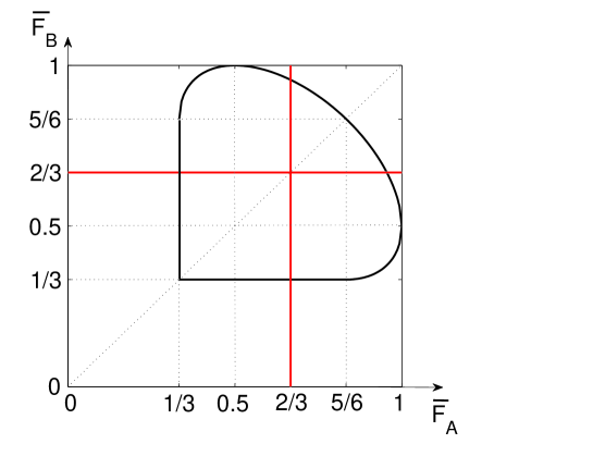
Figure 1: (Color online) The maximal and minimal average fidelity $\overline{F}_{B}$ of an interference free cloner as function of $\overline{F}_{A}$ (black line) enclose the convex domain of all possible interference–free cloners with positive dynamical matrix $D$. The maximum allowed classical fidelity for a symmetric cloner is $2/3$ (red lines).

V More general interference–free symmetric QCs

Semidefinite programming guarantees that a local optimum is also a global optimum. However, this does not exclude that other machines may exist with the same fidelity. Indeed, we shall show now that a high dimensional continuous class of symmetric QCs exists which all reach maximum average fidelity without making use of interference.

First observe that the dynamical matrix $D^{\rm opt}$ has eigenvalues 1 (doubly degenerate), $1/4$ (8 times degenerate), and 0 (6 times degenerate). Since $D^{\rm opt}$ is real and symmetric, its eigenvectors form a real orthogonal matrix $O$. The idea is then to add a hermitian perturbation $W$ to $D^{\rm opt}$ in the subspace of eigenvectors of $D^{\rm opt}$ corresponding to the non–vanishing eigenvalues, and which leaves the partial traces unchanged. If the perturbation is small enough, the positivity of $D^{\rm opt}$ cannot be jeopardized immediately. Furthermore, a perturbation can be easily constructed such that it is orthogonal to both ${\cal A}$ and ${\cal B}$ in the sense of the scalar product (9). Let $w_{IJ}$ be the matrix elements of $W$ ($0\leq I,J\leq 15)$ in the eigenbasis of $D^{\rm opt}$. Transformed back to the computational basis, $\widetilde{W}=OWO^{T}$, we find ${\cal A}\cdot\widetilde{W}$=${\cal B}\cdot\widetilde{W}$=$5(w_{00}+w_{11})/12$. Thus we have unmodified success probability $\overline{F}_{A}$ for

$$w_{11}=-w_{00}\,.$$ (16)

From the requirement of unchanged partial traces we get

$$w_{00}=w_{11} = 0$$ (17)

$$w_{3\,3}+w_{5\,5}+w_{7\,7}+w_{9\,9} = 0$$ (18)

$$w_{2\,2}+w_{4\,4}+w_{6\,6}+w_{8\,8} = 0\,.$$ (19)

The only thing which remains to be imposed is that transformed back to the computational basis the perturbation still has vanishing off–diagonal matrix elements on the diagonal blocks, in order to keep the interference at zero. This requires $w_{0\,1}$, $w_{0\,2}$, $w_{0\,3}$, $w_{0\,4}$, $w_{0\,5}$, $w_{0\,6}$, $w_{0\,7}$, $w_{1\,4}$, $w_{1\,5}$, $w_{1\,6}$, $w_{1\,7}$, $w_{1\,8}$, $w_{1\,9}$, $w_{2\,3}$, $w_{4\,5}$, $w_{6\,7}$, $w_{8\,9}$ to vanish. We are left with a large class of dynamical matrices $\widetilde{D}^{\rm opt}$ which can be written as a $4\times 4$ matrices of $4\times 4$ complex sub-blocks $\widetilde{D}^{\rm opt}_{I\,J}$ with $\widetilde{D}^{\rm opt}_{I\,J}=\left(\widetilde{D}^{\rm opt}_{J\,I}\right)^{{\dagger}}$ and $I,J\in\left\{0,\ldots,3\right\}$ where $\widetilde{D}^{\rm opt}_{0\,0}={\rm diag}\left(\frac{2}{3},\frac{1}{4}+w_{9\,9},0,\frac{1}{4}+w_{8\,8}\right)$, $\widetilde{D}^{\rm opt}_{1\,1}={\rm diag}\left(\frac{1}{6},\frac{1}{4}+w_{7\,7},\frac{1}{6},\frac{1}{4}+w_{6\,6}\right)$, $\widetilde{D}^{\rm opt}_{2\,2}={\rm diag}\left(\frac{1}{6},\frac{1}{4}+w_{5\,5},\frac{1}{6},\frac{1}{4}+w_{4\,4}\right)$, $\widetilde{D}^{\rm opt}_{3\,3}={\rm diag}\left(0,\frac{1}{4}+w_{3\,3},\frac{2}{3},\frac{1}{4}+w_{2\,2}\right)$ and

$$\widetilde{D}^{\rm opt}_{0\,1}=\left(\begin{array}[]{cccc}0&0&\frac{1}{3}&0\\ \frac{w_{0\,9}^{*}}{\sqrt{6}}&w_{7\,9}^{*}&0&w_{6\,9}^{*}\\ 0&0&0&0\\ \frac{w_{0\,8}^{*}}{\sqrt{6}}&w_{7\,8}^{*}&0&w_{6\,8}^{*}\\ \end{array}\right),\,\,\,\widetilde{D}^{\rm opt}_{0\,2}=\left(\begin{array}[]{cccc}0&0&\frac{1}{3}&0\\ \frac{w_{0\,9}^{*}}{\sqrt{6}}&w_{5\,9}^{*}&0&w_{4\,9}^{*}\\ 0&0&0&0\\ \frac{w_{0\,8}^{*}}{\sqrt{6}}&w_{5\,8}^{*}&0&w_{4\,8}^{*}\\ \end{array}\right)\,,$$ (20)

$$\widetilde{D}^{\rm opt}_{0\,3}=\left(\begin{array}[]{cccc}0&\sqrt{\frac{2}{3}}w_{1\,3}&0&\sqrt{\frac{2}{3}}w_{1\,2}\\ 0&w_{3\,9}^{*}&\sqrt{\frac{2}{3}}w_{0\,9}^{*}&w_{2\,9}^{*}\\ 0&0&0&0\\ 0&w_{3\,8}^{*}&\sqrt{\frac{2}{3}}w_{0\,8}^{*}&w_{2\,8}^{*}\\ \end{array}\right),\,\,\,\widetilde{D}^{\rm opt}_{1\,2}=\left(\begin{array}[]{cccc}\frac{1}{6}&0&0&0\\ 0&w_{5\,7}^{*}&0&w_{4\,7}^{*}\\ 0&0&\frac{1}{6}&0\\ 0&w_{5\,6}^{*}&0&w_{4\,6}^{*}\\ \end{array}\right)\,,$$ (21)

$$\widetilde{D}^{\rm opt}_{1\,3}=\left(\begin{array}[]{cccc}0&0&\frac{1}{3}&0\\ 0&w_{3\,7}^{*}&0&w_{2\,7}^{*}\\ 0&\frac{w_{1\,3}}{\sqrt{6}}&0&\frac{w_{1\,2}}{\sqrt{6}}\\ 0&w_{3\,6}^{*}&0&w_{2\,6}^{*}\\ \end{array}\right),\,\,\,\widetilde{D}^{\rm opt}_{2\,3}=\left(\begin{array}[]{cccc}0&0&\frac{1}{3}&0\\ 0&w_{3\,5}^{*}&0&w_{2\,5}^{*}\\ 0&\frac{w_{1\,3}}{\sqrt{6}}&0&\frac{w_{1\,2}}{\sqrt{6}}\\ 0&w_{3\,4}^{*}&0&w_{2\,4}^{*}\\ \end{array}\right)\,.$$ (22)

They depend on 64 real parameters, which, when taken small enough, leave $\widetilde{D}^{\rm opt}$ positive. We have thus found a large continuous class of symmetric interference–free QCs with maximum average fidelity $5/6$. It turns out that all these machines are also universal. This is a consequence of imposing zero interference, as is easily checked by relaxing this condition (see the discussion of vanishing matrix elements $w_{ij}$ after eq.(19)).

VI Comparison with the Bužek–Hillery QC

The comparison with the BH QC is not as straightforward as it may seem. The reason is that BH only specify what happens to a state $|\psi\rangle\otimes|0\rangle$, but the fate of $|\psi\rangle\otimes|1\rangle$ remains unspecified. In other words, only part of the dynamical matrix is defined, and in order to compare our interference–free QCs with the one by BH on the basis of the dynamical matrix, we would have to extend the definition of the BH QC to deal with the input state $|1\rangle$ for the second qubit as well. If we choose a natural extension,

$$|0\rangle_{a}|1\rangle_{b}|Q\rangle_{x} \rightarrow |0\rangle_{a}|1\rangle_{b}|Q_{2}\rangle_{x}+\left(|0\rangle_{a}|0\rangle_{b}+|1\rangle_{a}|1\rangle_{b}\right)|Y_{2}\rangle_{x}$$

$$|1\rangle_{a}|1\rangle_{b}|Q\rangle_{x} \rightarrow |1\rangle_{a}|0\rangle_{b}|Q_{3}\rangle_{x}+\left(|0\rangle_{a}|0\rangle_{b}+|1\rangle_{a}|1\rangle_{b}\right)|Y_{3}\rangle_{x}\,,$$ (23)

where the subscript $x$ denotes states of the cloner, unitarity imposes the same constraints as in eq.(3.3) in Bužek and Hillery (1996), but extended to $i=0,\ldots,3$. With an appropriate choice of overlaps between the states of the cloner, one can show that the BH QC is a member of the continuous class of QCs with dynamical matrices $\widetilde{D}^{\rm opt}$ found above. Alternatively, we can compare the QCs on the basis of the output reduced density matrices $\rho_{A}^{\prime}$ and $\rho_{B}^{\prime}$ obtained for mapping states $|\psi\rangle\otimes|0\rangle$. Doing so, we find that all optimal symmetric interference–free QCs with dynamical matrices $\widetilde{D}^{\rm opt}$ give the same single–qubit reduced matrix as the BH QC,

$${\rho_{A}^{\prime}}={\rho_{B}^{\prime}}=\left(\begin{array}[]{cc}\frac{2}{3}\left|\alpha\right|^{2}+\frac{1}{6}&\frac{2}{3}\alpha\beta^{*}\\ \frac{2}{3}\alpha^{*}\beta&\frac{5}{6}-\frac{2}{3}\left|\alpha\right|^{2}\\ \end{array}\right)\,,$$ (24)

with $\rho_{A}^{\prime}={\rm Tr}_{B}\left[\rho_{AB}^{\prime}\right]$, $\rho_{B}^{\prime}={\rm Tr}_{A}\left[\rho_{AB}^{\prime}\right]$ and $\rho_{AB}^{\prime}=\widetilde{D}^{\rm opt}|\psi\rangle\langle\psi|\otimes|0\rangle\langle 0|$.

VII Conclusion

We have found a large class of 1 $\to$ 2 qubit cloners, which outperform classical symmetric cloning of qubits in terms of the average fidelities, but do not use any interference in the effective map of the two qubits. In particular we find QCs which reproduce the optimal average fidelities 5/6 of symmetric universal QCs without using interference. The well–known Bužek–Hillery QC turns out to be a member of this general class of interference–free QCs. How is it possible that interference–free quantum cloning outperforms classical quantum cloning? The answer is clear from the structure of the dynamical matrices $D$: Classical cloning corresponds to a diagonal $D$, quantum cloning to a potentially full matrix $D$. Interference–free quantum cloning is situated somewhere in between — only the off–diagonals of the diagonal blocks need to vanish. In other words, interference–free propagation of the density matrix does not map any coherences (i.e. off-diagonal elements of the density matrix) to probabilities, but may well map coherences to other coherences. The latter process influences the fidelities, and the corresponding matrix elements can be used to optimize the fidelities beyond classically possible values. It is intriguing to find that for optimal quantum cloning (in the case of a $1\to 2$ qubit cloner) just this happens: only probabilities are mapped to probabilities, whereas coherences never modify the probabilities. It would be interesting to find out if this generalizes to higher dimensional or multiple–copy quantum cloning. It is also worthwhile noting that we have considered here the interference in the effective propagation of the two qubit system (original and copy). More general settings could be envisaged, for example including the copying machine as well. Additional information about the copying machine is needed then, however, and the results may depend on the dimension of the Hilbert space of the machine itself.

Acknowledgments: We thank CALMIP (Toulouse) and IDRIS (Orsay) for the use of their computers. This work was supported by the Agence National de la Recherche (ANR), project INFOSYSQQ, and the EC IST-FET project EUROSQIP. B. Roubert is supported by a grant from the DGA, with M. Jacques Blanc–Talon as scientific liaison officer.

References

- Wootters and Zurek (1982) W. K. Wootters and W. H. Zurek, Nature 299, 802 (1982).
- Aspect et al. (1982) A. Aspect, J. Dalibard, and G. Roger, Phys. Rev. Lett. 49, 1804 (1982).
- Weihs et al. (1998) G. Weihs, T. Jennewein, C. Simon, H. Weinfurter, and A. Zeilinger, Phys. Rev. Lett. 81, 5039 (1998).
- Aspect (1999) A. Aspect, Nature 398, 189 (1999).
- Rowe et al. (2001) M. A. Rowe, D. Kielpinski, V. Meyer, C. A. Sackett, W. M. Itano, C. Monroe, and D. J. Wineland, Nature 409, 791 (2001).
- Bužek and Hillery (1996) V. Bužek and M. Hillery, Phys. Rev. A 54, 1844 (1996).
- Gisin and Massar (1997) N. Gisin and S. Massar, Phys. Rev. Lett. 79, 2153 (1997).
- Bruß et al. (1998) D. Bruß, D. P. DiVincenzo, A. Ekert, C. A. Fuchs, C. Macchiavello, and J. A. Smolin, Phys. Rev. A 57, 2368 (1998).
- Gisin (1998) N. Gisin, J. Phys. A 242, 1 (1998).
- Horodecki et al. (1999) M. Horodecki, P. Horodecki, and R. Horodecki, Phys. Rev. A 60, 1888 (1999).
- Scarani et al. (2005) V. Scarani, S. Iblisdir, N. Gisin, and A. Acin, Reviews of Modern Physics 77, 1225 (pages 32) (2005).
- Bennett and DiVincenzo (2000) C. H. Bennett and D. P. DiVincenzo, Nature 404, 247 (2000).
- Bruß and Macchiavello (2003) D. Bruß and C. Macchiavello, Foundations of Physics 33, 1617 (2003).
- Braun and Georgeot (2006) D. Braun and B. Georgeot, Phys. Rev. A 73, 022314 (2006).
- Braun and Georgeot (2008) D. Braun and B. Georgeot, Physical Review A (Atomic, Molecular, and Optical Physics) 77, 022318 (2008).
- Arnaud and Braun (2007) L. Arnaud and D. Braun, Physical Review A (Atomic, Molecular, and Optical Physics) 75, 062314 (2007).
- Lyakhov et al. (2007) A. O. Lyakhov, D. Braun, and C. Bruder, Physical Review A (Atomic, Molecular, and Optical Physics) 76, 022321 (2007).
- Życzkowski and Bengtsson (2004) K. Życzkowski and I. Bengtsson, Open Syst. Inf. Dyn. 11 11, 3 (2004).
- Barnum et al. (1996) H. Barnum, C. M. Caves, C. A. Fuchs, R. Jozsa, and B. Schumacher, Phys. Rev. Lett. 76, 2818 (1996).
- Choi (1975) M.-D. Choi, Linear Alg. Appl. 10, 285 (1975).