Pure cross-diffusion models:
Implications for traveling wave solutions

Abstract

An analysis of traveling wave solutions of pure cross-diffusion systems, i.e., systems that lack reaction and self-diffusion terms, is presented. Using the qualitative theory of phase plane analysis the conditions for existence of different types of wave solutions are formulated. In particular, it is shown that family of wave trains is a generic phenomenon in pure cross-diffusion systems. The results can be used for construction and analysis of different mathematical models describing systems with directional movement.

Keywords:

PDE systems, cross-diffusion, traveling waves, traveling trains, taxis

AMS (MOS) subject classification:

34C05, 34C25, 35Q80, 92C17

1 Introduction

Using so-called cross-diffusion terms in mathematical models in natural sciences, in particular in biology, is nowadays a routine trick to incorporate into classical models additional effects such as taxis movement, crowding, pursuit, or evasion (for a review see [18]). Two particular examples, which received especial attention amongst other models, are the Keller–Segel model of chemotactic movement [17, 12, 10] (taxis is defined as behavioral response to a directional stimulus), and the Lotka–Volterra type cross-diffusion model to describe predator pursuit of an evading prey [13, 11, 7, 9].

A distinct feature of many studies on cross-diffusion models (PDE systems where diffusion matrix is not diagonal) is that usually a particular model is analyzed, where terms of reaction and diffusion coefficients are given in fixed explicit form; notable exceptions are given by [3, 10, 5]. It also appears that almost all the models considered contain reaction terms, only one exception we know of notwithstanding [8], although it might be argued that systems without reaction terms possess numerous solutions which may be relevant in biological modeling.

Taking a step further, in this note we consider the systems that lack the self-diffusion terms; PDE systems we analyze possess only cross-diffusion (as, e.g., in [6, 14], but with nonlinear cross-diffusion coefficients). We dub such systems without reaction and self-diffusion terms pure cross-diffusion systems. In particular, we study the PDE system in the following form:

$$\begin{split}u_{t}&=d_{1}(f(u,v)v_{x})_{x},\\ v_{t}&=d_{2}(g(u,v)u_{x})_{x},\end{split}$$ (1)

where $u=u(x,t),\,v=v(x,t),\,-\infty<x<\infty,\,t\geqslant 0,$ $d_{1},d_{2}$ are real constants, and $f(u,v),\,g(u,v)$ are arbitrary functions whose properties will be specified later. Qualitatively system (1) describes mutually dependent movement of conserved entities $u$ and $v$ on gradients of their respective counterparts. Of particular interest for us are the traveling wave solutions of system (1), which, e.g., can describe a replacement process of one species by another species. As usual, a wave solution of (1) is a bounded solution having the form $u(x,t)=u(x+ct)=u(\xi),\,v(x,t)=v(x+ct)=v(\xi)$, where $c$ is the wave speed. On substituting these traveling wave forms into (1) we obtain the ODE wave system

$$\begin{split}cu_{\xi}&=d_{1}(f(u,v)v_{\xi})_{\xi},\\ cv_{\xi}&=d_{2}(g(u,v)u_{\xi})_{\xi}.\end{split}$$ (2)

Note that we can integrate system (2), and therefore, (2) is essentially two dimensional, as the original PDE system. Each wave solution of (1) has its counterpart as a bounded orbit of (2), which, due to the particular structure of (2), is an orbit on a phase plane. There is a known correspondence between wave solutions of (1) and bounded orbits of (2): A wave front in, e.g., $u$ component corresponds to a heteroclinic orbit of (2) that connects singular points with different $u$ coordinates; A wave impulse in, e.g., $u$ component corresponds to a heteroclinic orbit of (1) that connects singular points with identical $u$ coordinates or to a homoclinic curve of a singular point; A wave train corresponds to a closed orbit of system (2).

In the next section we show that, under some natural restrictions on functions $f(u,v)$ and $g(u,v)$, all possible traveling wave solutions of (1) can be classified. In particular, a family of wave trains of (1) is a generic phenomenon intrinsic to (1). Section 3 provides some examples and extensions. Section 4 is devoted to discussion and conclusions.

2 Wave solutions of the separable models

In this note we confine ourselves to a particular case of (1), whereby the functions $f(u,v)$ and $g(u,v)$ can be represented as products of functions that depend on one variable:

$$f(u,v)=f_{1}(u)f_{2}(v),\,g(u,v)=g_{1}(u)g_{2}(v).$$ (3)

Here the functions $f_{i}(x),\,g_{i}(x),\,i=1,2$ are smooth or rational. The models of the form (1) for which (3) holds will be termed separable pure cross diffusion models, or separable models for short.

The rationale behind the choice of the from of the functions $f$ and $g$ as in (3) is twofold. Firstly, such assumption allows complete analysis of possible structures of the corresponding wave system, and thus, exhaustive classification of possible wave solutions of (1) as was done for different models in [5, 4]. Secondly, such forms are abundant in the modeling literature being the consequence of a biased random walk on the lattice (see, e.g., [16]).

For the separable model and after integration and rearrangement wave system (2) takes the form

$$\begin{split}u_{\xi}&=cd_{2}(v-\eta)/g(u,v),\\ v_{\xi}&=cd_{1}(u-\mu)/f(u,v),\end{split}$$ (4)

where $c\eta,\,c\mu$ are constants of integration that in general depend on boundary conditions, and which are considered here as new parameters of the system (see also [5]). After the change of independent variable

$$d\zeta=\frac{cd\xi}{d_{1}d_{2}f(u,v)g(u,v)}\,,$$

which is well defined and smooth for any $(u,v)$ except where $f(u,v)g(u,v)=0$ or where $f(u,v)$ or $g(u,v)$ are not defined (see [1]), we obtain

$$\begin{split}u_{\zeta}&=d_{1}f_{1}(u)f_{2}(v)(v-\eta),\\ v_{\zeta}&=d_{2}g_{1}(u)g_{2}(v)(u-\mu).\end{split}$$ (5)

In the case if $f(u,v)$ or $g(u,v)$ are rational, the change of independent variable is chosen such that the resulting wave system is well defined for all $u$, $v$ (for examples see the next section). Therefore, without loss of generality, we assume that our wave system has the form

$$\begin{split}u_{\zeta}&=d_{1}\varphi_{1}(u)\varphi_{2}(v)(v-\eta),\\ v_{\zeta}&=d_{2}\psi_{1}(u)\psi_{2}(v)(u-\mu).\end{split}$$ (6)

which is defined for all $u,\,v$.

First we note that system (6) is integrable. Function

$$H(u,v)=d_{1}\int(v-\eta)\frac{\varphi_{2}(v)}{\psi_{2}(v)}\,dv-{d_{2}}\int(u-\mu)\frac{\psi_{1}(u)}{\varphi_{1}(u)}\,du+\mbox{const}$$

represents its integral. We remark that under the assumption $\varphi_{1}(u)=\mbox{const},\,\psi_{2}(v)=\mbox{const}$ system (6) is hamiltonian, and $H(u,v)$ is its Hamiltonian, which automatically yields that the singular points of (6) can be only topological saddles or centers.

We assume that the following conditions of non-degeneracy are fulfilled (these conditions are natural as far as we consider $\eta,\,\mu,\,c$ the only parameters in the system (6)):

$$\begin{split}(C1)&\quad\mbox{$\varphi_{1}(u)$ and $\psi_{1}(u)$ have no common roots;}\\ (C2)&\quad\mbox{$\varphi_{2}(v)$ and $\psi_{2}(v)$ have no common roots;}\\ (C3)&\quad\mbox{$\varphi_{i}(x)$ and $\psi_{i}(x),\,i=1,2,$ have no multiple roots.}\end{split}$$

System (6) always has singular point $(\mu,\,\eta)$. Coordinates of other singular points are $(\mu,\hat{v}_{i}),\,(\hat{u}_{i},\,\eta),\,(\hat{u}_{i},\hat{v}_{i})$, where $\hat{u}_{i}$ and $\hat{v}_{i}$ are the solutions of one of the systems:

$$\varphi_{1}(u)=0,\quad\psi_{2}(v)=0,$$ (7)

or

$$\varphi_{2}(v)=0,\quad\psi_{1}(u)=0.$$ (8)

To infer the possible types of the singular points of (6) consider the Jacobi matrix of (6): $DF(u,v)=(a_{ij})_{2\times 2},\,i,j=1,2$:

$$\begin{split}a_{11}&=d_{1}(v-\eta)\varphi_{2}(v)(\varphi_{1}(u))^{\prime}_{u},\\ a_{12}&=d_{1}\varphi_{1}(u)((v-\eta)(\varphi_{2}(v))^{\prime}_{v}+\varphi_{2}(v)),\\ a_{21}&=d_{2}\phi_{2}(v)((u-\mu)(\psi_{1}(u))^{\prime}_{u}+\psi_{1}(u)),\\ a_{22}&=d_{2}(u-\mu)\psi_{1}(u)(\psi_{2}(v))^{\prime}_{v}.\end{split}$$ (9)

Direct substitution of singular point coordinates into (9) and evaluation of trace and determinant of $DF$ implies the following proposition.

Proposition 1.

Let us assume that conditions $(C1)$–$(C3)$ hold. We also assume that $\hat{u}_{i}$ ($\hat{v}_{i}$) do not coincide with $\mu$ ($\eta$, respectively). Then

1. Singular points of (6) satisfying (7) or (8) can be saddles or nodes only;

2. Singular points of (6) where one or both coordinates are $\eta$ or $\mu$ can be centers or saddles only.

Remark 1.

If we relax condition $(C3)$ retaining $(C1)$ and $(C2)$ then we have to add to the list of possible singular points of (6) saddle-node points.

Remark 2.

To prove that singular points that have eigenvalues with zero real part in linear approximation are indeed centers we can use integrability of system (6) and Theorem 2 in [2, p. 75].

From Proposition 1, integrability of system (6), and special structure of the wave system (6) follows that the structure of the phase plane, and, consequently, of the bounded orbits of (6) are completely determined by the types and mutual positions of singular points of (6). The phase plane is divided into orbit cells that represent either a rectangular cell with orbit structure determined by the types of the corner singular points (as in [5]), or a cell filled with closed orbits surrounding singular point of the center type (an example of such phase plane is given in Fig. 1). The former case corresponds to fronts or impulses of the initial system (1), and the latter to the wave train solutions of system (1).

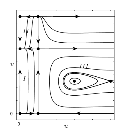
Figure 1: A typical structure of the phase plane of the wave system of the separable model (1). Here the bold dots represent singular points of (6), the arrows show direction of the vector field. The plane is divided into orbit cells that contain families of bounded orbits: $I$ is a cell that corresponds to impulse-front solutions; $II$ is a cell that corresponds to front-front solutions; $III$ is a cell that corresponds to traveling train solutions, the homoclinic surrounding the closed orbits corresponds to impulse-impulse solutions

Summarizing, we obtain the basic result of the present note:

Theorem 1.

The separable pure cross-diffusion system (1), satisfying $(C1)$–$(C3)$ can only possess traveling wave solutions of the following kinds: i. impulse-front solutions; ii. front-front solutions; iii. impulse-impulse solutions; iv. family of wave train solutions.

The family of wave train solutions exits in domain $\Omega$ if $f(u,v)$ and $g(u,v)$ are analytical in $\Omega$ and $d_{1}d_{2}f(u,v)g(u,v)<0$ for $(u,v)\in\Omega$.

3 Examples

Example 1.

The simplest possible separable model (1) is obtained if we put

$$f_{1}(u)=f_{2}(v)=g_{1}(u)=g_{2}(v)=1.$$ (10)

The integral in this case is given by

$$d_{2}(u-\mu)^{2}-d_{1}(v-\eta)^{2}=\mbox{const}.$$

From which it follows that system (1) with (10) has no traveling wave solution if $d_{1}d_{2}>0$ and has a family of traveling trains if $d_{1}d_{2}<0$.

Remark.

Note that in case $d_{1}d_{2}<0$ system (1) is equivalent to the beam equation $u_{tt}=-Du_{xxxx},\,D>0$, which, how it is well known, possesses wave solutions.

Example 2.

Let

$$\begin{split}f_{2}(v)&=g_{1}(u)=\mbox{const}\\ f_{1}(u)&=(u-a)^{n},\,g_{2}(v)=(v-b)^{m},\,n,m\in\mathbb{N}.\end{split}$$ (11)

It is straightforward to prove

Proposition 2.

Separable model (1) with (11) has a family of wave trains if $d_{1}d_{2}<0$ and has a front-front solution, that corresponds to a heteroclinic connecting node and saddle, if $d_{1}d_{2}>0$.

Example 3.

Let

$$\begin{split}f_{1}(u)&=u^{n},\,f_{2}(v)=\frac{1}{v^{m}}\,,\\ g_{1}(u)&=\frac{1}{u^{n}}\,,\,g_{2}(v)=v^{m},\end{split}$$ (12)

where $m,n\in\mathbb{N}$. After a suitably chosen change of independent variable in the wave system (4) we obtain

$$\begin{split}u_{\zeta}&=d_{1}u^{2n}(v-\eta),\\ v_{\zeta}&=d_{2}v^{2m}(u-\mu).\end{split}$$ (13)

Having in mind biological applications of the pure cross-diffusion models we assume that $\mu>0,\,\eta>0$ and analyze the phase plane in the first quadrant. System (13) has two singular points: $(0,0)$ and $(\mu,\,\eta)$. The point $(\mu,\,\eta)$ can be a saddle (if $d_{1}d_{2}>0$) or a center ($d_{1}d_{2}<0$). If we restrict our attention only to the cases $\mu>0,\,\eta>0$, $u,v>0$, then traveling wave solutions of (1) with (13) are exactly the same as in Proposition 2.

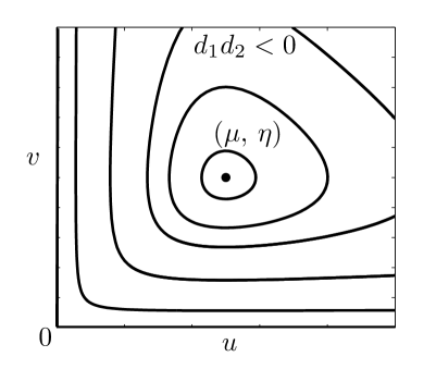
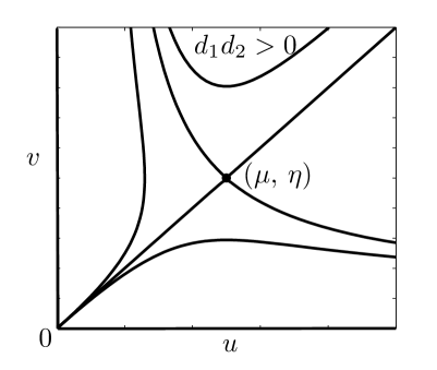
Figure 2: The structure of the first quadrant of the phase plane of the wave system (2), (12). In case $d_{1}d_{2}<0$ a family of closed orbits can be found, which corresponds to the wave trains; in case $d_{1}d_{2}>0$ there is only one bounded trajectory that connect the origin and the saddle point $(\mu,\,\eta)$

Let us illustrate this case. In Fig. 2 the first quadrant of the phase plane of the wave system of (1),(12) is shown for two topologically nonequivalent cases. The first case corresponds to the wave train in the original PDE system, and the second case corresponds to front-front solution. In Fig. 3 numerically obtained solutions of (1),(12) are presented. To approximate cross-diffusion term an “upwind” explicit scheme was used [15] which is often used for cross-diffusion systems (e.g., [19]).

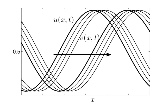
Figure 3: Numerically obtained wave train solutions of system (1),(12) at time moments $t_{0}=0$(bold curves)$<t_{1}<t_{2}<t_{3}$ through equal time intervals. The arrow shows the direction of the waves

Example 4.

We can use obtained results to prove existence of solutions of a special form when simple reaction terms are presented. For example, let us consider the following system:

$$\begin{split}u_{t}&=b_{1}u+d_{1}(u^{n}/v^{m}v_{x})_{x},\\ v_{t}&=b_{2}v+d_{2}(v^{m}/u^{n}u_{x})_{x}.\end{split}$$ (14)

If the constant $b_{1},\,b_{2},\,n,\,m$ satisfy the following equality:

$$b_{1}(1-n)=b_{2}(1-m),$$

then by the change

$$u(x,t)=e^{b_{1}t}z(z,t),\,v(x,t)=e^{b_{2}t}w(x,t)$$

system (14) can be reduced to system (1), (12). Thus system (14) has wave train solutions with amplitude changing with time. It is interesting to note that for some models of the form (14) an exact solution can be found.

Example 5.

Consider the system

$$\begin{split}u_{t}&=u+d_{1}v_{xx},\\ v_{t}&=-\gamma v+d_{2}u_{xx}.\end{split}$$ (15)

Proposition 3.

For $\gamma<1$ and $d_{1}+d_{2}>0$ system (15) has a family of wave trains.

Proof.

We will prove proposition by presenting a solution of (15) in explicit form.

Let $u(\xi)=\cos k\xi,\,v(\xi)=\sin k\xi,\,\xi=x+ct$. Then system (15) transforms to the equations

$$\begin{split}-ck\sin k\xi&=\sin k\xi-d_{1}k^{2}\sin k\xi,\\ ck\cos k\xi&=-\gamma\cos k\xi-d_{2}k^{2}\cos k\xi,\end{split}$$

from which

$$\begin{split}d_{1}k^{2}-ck-1&=0,\\ d_{2}k^{2}+ck+\gamma&=0\end{split}$$

follows. For fixed $d_{1},\,d_{2},\,\gamma$ the solution of the last system is given by

$$k=\frac{\sqrt{1-\gamma}}{d_{1}+d_{2}},\,c=-\frac{d_{2}+d_{1}\gamma}{\sqrt{(d_{1}+d_{2})(1-\gamma)}},$$

which is defined for $\gamma<1$ and $d_{1}+d_{2}>0$, which completes the proof. ∎

Example 6.

An obvious question is what kind of solutions can appear in pure cross-diffusion models if we do not demand that the functions $f(u,v)$ and $g(u,v)$ can be represented as the product of functions of one variable. Despite the fact that the separable models possess very reach structure of possible traveling wave solutions, simple extension of the models considered can be shown to yield a different type of behavior.

Consider the model (1) with the functions given by

$$\begin{split}f(u,v)&=\frac{u}{\alpha u+v},\\ g(u,v)&=\frac{v}{u+\beta v},\end{split}$$ (16)

where $\alpha$ and $\beta$ are positive constant.

The wave system, after suitable change of independent variable, reads

$$\begin{split}u_{\zeta}&=d_{1}(v-\eta)u(\alpha u+\eta),\\ v_{\zeta}&=d_{2}(u-\mu)v(u+\beta v).\end{split}$$ (17)

Assume that all the parameters, except for $d_{1},\,d_{2}$ are positive. Singular point $(\mu,\,\eta)$ is a saddle, if $d_{1}d_{2}>0$ and a center at linear approximation for $d_{1}d_{2}<0$. However, contrast to model in Example 3, and due to the fact that the wave system is now non-integrable, we cannot make conclusion on the type of the singular point in the case $d_{1}d_{2}<0$. If we calculate the first Lyapunov value $l_{1}$ [2], we obtain $l_{1}=d_{1}d_{2}\mu\eta(\alpha\beta-1)(\alpha\mu^{2}-\beta\eta^{2})$, which shows that for parameter values where $l_{1}\neq 0$ this singular point can be either stable or unstable nonlinear focus.

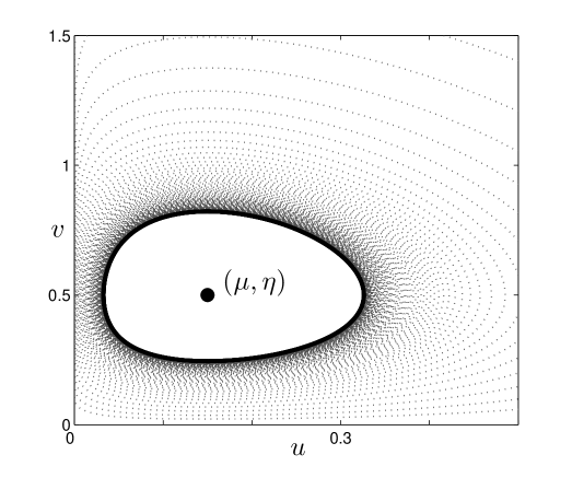
Figure 4: Limit cycle in the wave system (17). Parameter values $d_{1}=-1,\,d_{2}=1,\,\alpha=0.7,\,\beta=0.2,\,\mu=0.3,\,\eta=0.5$

Numerical experiments show that at least for some parameter values there is a limit cycle surrounding the singular point (see Fig. 4). Thus, in this example, there is a wave train solution of the initial pure cross-diffusion system.

4 Conclusions

In the present note we have shown that pure cross-diffusion models possess very rich structure of possible traveling wave solutions even in a rather simplified, though still realistic, case of separable models, when the nonlinear cross-diffusion coefficients in system (1) can be represented by product of functions depending on one variable.

A distinct feature of pure cross diffusion models is the presence, under some additional condition, of the family of wave train solutions (such solutions were not found for several classed of cross-diffusion models describing taxis, see [5, 4]). As numerical experiments show, such wave trains can be observed at least for some time interval. Together with families of wave trains, other typical cases of traveling waves can be observed. In particular, impulse-front, front-front, and impulse-impulse solutions are also a possibility.

We emphasize that the separable model (1), even when the values of parameters $\mu,\eta,c$ are fixed, possesses, in general, a family of traveling wave solutions; there are infinitely many bounded orbits of (2) that correspond to traveling wave solutions.

The presented results can be used for construction and analysis of different mathematical models describing systems where directional movement is of particular importance.

References

- [1] A. A. Andronov, E. A. Leontovich, I. I. Gordon, and A. G. Maier. Qualitative theory of second-order dynamic systems. Translated from Russian by D. Louvish. A Halsted Press Book, 1973.
- [2] N. N. Bautin and E. A. Leontovich. Methods and means for a qualitative investigation of dynamical systems on the plane. Nauka, 2d edition, 1990. In Russian.
- [3] F. S. Berezovskaya and G. P. Karev. Bifurcations of travelling waves in population taxis models. Uspekhi Fizicheskikh Nauk, 169(9):1011–1024, 1999.
- [4] F. S. Berezovskaya, A. S. Novozhilov, and G. P. Karev. Traveling fronts, impulses and trains in some taxis models. Neural, Parallel and Scientific Computations, 15(4):561–571, 2007.
- [5] F. S. Berezovskaya, A. S. Novozhilov, and G. P. Karev. Families of traveling impulses and fronts in some models with cross-diffusion. Nonlinear Analysis: Real World Applications, 2008, in press.
- [6] J. H. E. Cartwright, E. Hernandez-Garcia, and O. Piro. Burridge – Knopoff Models as Elastic Excitable Media. Physical Review Letters, 79(3):527–530, 1997.
- [7] B. Dubey, B. Das, and J. Hussain. A predator-prey interaction model with self and cross-diffusion. Ecological Modelling, 141(1-3):67–76, 2001.
- [8] K. P. Hadeler. Cross Diffusion and Coexistence of two species on a gradient. Canadian Applied Mathematics Quarterly, 15(2):169–180, 2007.
- [9] D. Horstmann. Remarks on some Lotka–Volterra type cross-diffusion models. Nonlinear Analysis: Real World Applications, 8(1):90–117, 2007.
- [10] D. Horstmann and A. Stevens. A constructive approach to traveling waves in chemotaxis. Journal of Nonlinear Science, 14(1):1–25, 2004.
- [11] J. Jorne. The diffusive Lotka-Volterra oscillating system. Journal of Theoretical Biology, 65(1):133–139, 1977.
- [12] E. F. Keller and L. A. Segel. Model for Chemotaxis. Journal of Theoretical Biology, 30(2):225–234, 1971.
- [13] E. H. Kerner. Further considerations on statistical mechanics of biological assosiation. Bulletin of Mathematical Biophysics, 21:217–255, 1959.
- [14] Yu. A. Kuznetsov, M. Y. Antonovsky, V. N. Biktashev, and E. A. Aponina. A cross-diffusion model of forest boundary dynamics. Journal of Mathematical Biology, 32(3):219–232, 1994.
- [15] K. W. Morton and D. F. Mayers. Numerical Solution of Partial Differential Equations: An Introduction. Cambridge University Press, 2005.
- [16] H. G. Othmer and A. Stevens. Aggregation, blowup, and collapse: The ABC’s of taxis in reinforced random walks. Siam Journal on Applied Mathematics, 57(4):1044–1081, 1997.
- [17] C. S. Patlak. Random walk with persistence and external bias. Bulletin of Mathematical Biology, 15(3):311–338, 1953.
- [18] M. A. Tsyganov, V. N. Biktashev, J. Brindley, A. V. Holden, and G. R. Ivanitsky. Waves in systems with cross-diffusion as a new class of nonlinear waves. Uspekhi Fizicheskikh Nauk, 177(3):275–300, 2007.
- [19] M. A. Tsyganov, J. Brindley, A. V. Holden, and V. N. Biktashev. Properties of population taxis waves in a predator prey system with pursuit and evasion. Physica D, 197:18–33, 2004.