A Radar for the Internet

Abstract

In contrast with most internet topology measurement research, our concern here is not to obtain a map as complete and precise as possible of the whole internet. Instead, we claim that each machine’s view of this topology, which we call ego-centered view, is an object worth of study in itself. We design and implement an ego-centered measurement tool, and perform radar-like measurements consisting of repeated measurements of such views of the internet topology. We conduct long-term (several weeks) and high-speed (one round every few minutes) measurements of this kind from more than one hundred monitors, and we provide the obtained data. We also show that these data may be used to detect events in the dynamics of internet topology.

1 Introduction.

Since the end of the nineties, constructing maps of the internet using traceroute-like measurements received much attention, see for instance [13, 26, 18, 3, 20, 14, 21, 7, 29, 16, 27]. Such measurements are however partial and they may contain significant bias [19, 6, 8, 9, 17, 4]. As a consequence, much effort is nowadays devoted to the collection of more accurate data [26, 3, 5, 28], but this task is challenging.

In order to avoid these issues and obtain some insight on internet topology dynamics, we use here a radically different approach: we focus on what a given machine sees of the topology around itself, which we call an ego-centered view (it basically is a routing tree measured in a traceroute-like manner). These ego-centered measurements may be performed very efficiently (typically in minutes, and inducing low network load); it is therefore possible to repeat them in periodic rounds, and obtain in this way information on the dynamics of the topology, at a time-scale significantly higher than previous approaches (see for instance [23, 8]).

Taking advantage of these strengths, we conduct massive radar-like measurements of the internet. We provide both the measurement tool and the collected data, and show that they reveal interesting features of the observed topology.

2 Measurement framework.

One may use traceroute directly to collect ego-centered views by probing a set of destinations. This approach however has serious drawbacks. First, as detailed in [11] and illustrated in Figure 1, the measurement load is highly unbalanced between nodes and there is much redundancy in the obtained data (intuitively, one probes links close to the monitor much more than others). Even worse, this implies that the obtained information is not homogeneous, and thus much more difficult to analyse rigorously (for instance, the dynamics may seem higher close to the monitor). Finally, though the measurement would intuitively produce a routing tree, the obtained view actually differs significantly from a tree (see for instance [28]). Again, this makes the analysis (visualisation of the data, for instance) more intricate.

Finally, the direct traceroute approach has multiple severe drawbacks. In this section we first design an ego-centered measurement tool remedying to this. We then include it in a radar measurement scheme.

2.1 Ego-centered measurements.

As already discussed in various contexts [12, 11, 10, 24, 22, 27], one may avoid the issues described above by performing tree-like measurements in a backward way: given a set of destinations to probe, one first discovers the last link on the path to each of them, then the previous link on each of these paths, and so on; when two (or more) paths reach the same node then the probing towards all corresponding destinations, except one, stops . However, as illustrated in Figure 1, naive such measurements encounter serious problems because of routing changes and other events. We provide a solution in the tracetree algorithm below: the tree nodes are not ip addresses anymore, but pairs composed of an ip address (or a star if a timeout occurred) and the ttl at which it was observed (see Figure 1 for an illustration). This is sufficient to ensure that the obtained view is a tree, while keeping the algorithm very simple. It sends only one packet for each link, and thus is optimal. Moreover, each link is discovered exactly once, which gives an homogeneous view of the topology and balances the measurement load.

Input: set $D$ of destinations, with $d\in D$ at distance $ttl_{d}$.

$to\_probe$ $\leftarrow$  empty queue, $to\_receive$ $\leftarrow$  $\emptyset$, $seen$ $\leftarrow$  $\emptyset$

foreach $d\in D$ do add $(d,ttl_{d})$ to $to\_probe$

while $to\_probe$ not empty or $to\_receive\not=\emptyset$ do  $\alpha$ if $to\_probe$ not empty then  pop $(d,ttl)$ from $to\_probe$ and send a probe to it

add $(d,ttl,current\_time())$ to $to\_receive$

  // here necessarily $to\_receive\not=\emptyset$

$\beta$       if answer $p$ to a probe to $(d,ttl)$ received then  // $p$ sent by $p.source$, reply to a probe to $(d,ttl)$

if $(d,ttl,\_)\in to\_receive$ then  // else timeout

remove $(d,ttl,\_)$ from $to\_receive$;

print $p.source$ $ttl$ $d$

if $(p.source,ttl)\not\in seen$ then  add $(p.source,ttl)$ to $seen$

push $(d,ttl-1)$ in $to\_probe$ if $ttl>1$

      for $(d,ttl,t)\in to\_receive$ if timeout exceeded do  remove $(d,ttl,t)$ from $to\_receive$

print * $ttl$ $d$

push $(d,ttl-1)$ in $to\_probe$ if $ttl>1$

   

Algorithm 1 tracetree algorithm.

Figure 1: Typical outputs of various measurements schemes. (1) – Real topology. $a$ is the monitor, $n$, $o$, and $p$ are the destinations. We suppose that $l$ does not answer to probes, that $b$ is a per-destination load balancer, forwarding traffic for $n$ to $d$, and traffic for $o$ to $f$, and that $e$ is a per-packet load balancer forwarding packets alternately to $i$ and $h$. Such situations are frequent in practice. (2) – Measurement with traceroute. Three routes are collected, leading to a higher load on links close to the monitor (represented by thicker lines here). (3) – Naive tree measurement. Because of a route change due to per-packet load balancer $e$, one obtains a disconnected part. (4) – Measurement with tracetree. Nodes are pairs of ip addresses and ttl, with redundancy in the addresses; one necessarily obtains a tree. (5–7) – Main steps of the filtering process. (5) – Pairs with same ip address are merged and loops are removed; (6) – Appropriate stars are merged and a bfs tree is computed; (7) – Leaves which are not the last node on a path towards a destination are iteratively removed. This is the final output of the filter.

From such trees with (ip,ttl) nodes, one obtains a tree on ip addresses by applying the following filter (illustrated in Figure 1) : first merge all nodes of the tree which correspond to a same ip; remove loops (links from an ip to itself); iteratively remove the stars with no successor; merge all the stars which are successor of a same node into a unique star; construct a bfs tree of the obtained graph which leads to a tree on ip addresses ; iteratively remove the leaves which are not the last nodes encountered when probing any destination.

The key point is that the obtained tree is a possible ip routing tree from the monitor to the destinations (similar to a broadcast tree). The obtained tree contains almost as much information as the original tracetree output and has the advantage of being much more simple to analyse. We evaluated the impact of this filtering on our observations, and found that it was negligible: Detailing this is out of the scope of this paper.

Many non-trivial points would deserve more discussion. For instance, one may apply a greedy sending or receiving strategy (by replacing line $\alpha$ or $\beta$ in Algorithm 1 by a while, respectively); identifying reply packets is non-trivial, as well as extracting the relevant information from the read packets; introducing a delay may be necessary to stay below the maximal icmp sending rate of the monitor; one may consider answers received after the timeout but before the end of the measurement (whereas we ignore them); one may use other protocols than icmp (the classical traceroute uses udp or icmp packets); the initial order of the destinations may have an impact on the measurement; there may be many choices for the bfs tree in the filter; etc. However, entering in such details is far beyond the scope of this paper, and we refer to the code and its documentation [2] for full details.

2.2 Radar.

With the tracetree tool and its filtered version, we have the ground material to conduct radar measurements: given a monitor and a set of destinations, it suffices to run periodic ego-centered measurements, which we call measurement rounds. The measurement frequency must be high enough to capture interesting dynamics, but low enough to keep the network load reasonable. We will discuss this in the next section.

The only remaining issue is the estimation of distances towards destinations, which is a non-trivial task in general [22]. This plays a key role here, since over-estimated distances lead to several packets hitting destinations. Under-estimated distances, instead, miss the last links towards the destinations.

One may however suppose that the distance between the monitor and any destination generally is stable between consecutive rounds of radar measurement. Then, the distances at a given round are the ones observed during the previous round. If the distance happens to be under-estimated (we do not see the destination at this distance), then we set it to a default maximal value (generally equal to $30$) and start the measurement from there (and we update the corresponding distance for the next round).

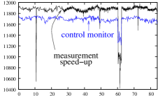
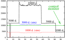
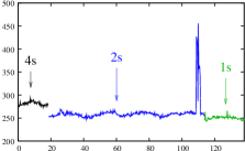
  $x$ = hours; $y$ = # ip   $x$ = hours; $y$ = # ip   $x$ = hours; $y$ = round duration (s)

Figure 2: Impact of measurement parameters. The $x$ axis of all plots represents the time (in hours) since the beginning of the measurement. Left: impact of inter-round delay. Number of distinct ip addresses viewed at each round. The bottom plot corresponds to a control monitor with the base parameters; the other monitor starts with the base parameters, and about $27$ hours later we reduce the inter-round delay from $10$ minutes to $1$ (each ego-centered measurement takes around $4$ minutes). Center: impact of the number of destinations. Number of distinct ip addresses viewed at each round. The plot close to $y=10\,000$ corresponds to a control monitor with the base parameters. The other plain-line plot is produced by a monitor which starts with the base parameters, thus with a destination set $D$ of size $3\,000$, changes to a set $D^{\prime}$ of $10\,000$ destinations containing $D$, goes back to $D$, and finally turns to a subset $D^{\prime\prime}$ of size $1\,000$ of $D$. In addition, the dotted plots are simulations of what we would have seen from this monitor with $D$ during the measurement using $D^{\prime}$ (obtained by dropping all nodes and links which are on paths towards destinations that are not in $D$), and what we would have seen with $D^{\prime\prime}$ during the measurements using $D$ or $D^{\prime}$ (obtained similarly). Right: impact of timeout value. Round duration (in seconds). The monitor starts with a timeout value of $4\,s$, then we change it to $2\,s$, and finally to $1\,s$.

3 Measurement and data.

First notice that many parameters (including the monitor and destination set) may have a deep impact on the obtained data. Estimating this impact is a challenging task since testing all combinations of parameters is totally out of reach. In addition, the continuous evolution of the measured object makes it difficult to compare several measurements: the observed changes may be due to parameter modifications or to actual changes in the topology.

To bypass these issues while keeping the study rigorous, we propose the following approach. We first choose a set of seemingly reasonable parameters, which we call base parameters (see Section 3.1). Then we conduct measurements with these parameters from several monitors in parallel. On some monitors, called control monitors, we keep these parameters constant; on others, called test monitors, we alternate periods with base parameters and periods where we change (generally one of) these parameters. Control monitors make it possible to check that the changes observed from test monitors are due to changes of parameters, not to events on the network. The alternation of periods with base parameters and modified ones also makes it possible to confirm this, and to observe the induced changes in the observations. In many cases, it is also possible to simulate what one would have seen in principle if the parameters had stayed unchanged, which gives further insight (we will illustrate this below).

We use a wide set of more than one hundred monitors scattered around the world, provided by PlanetLab [25] and other structures (small companies and individual dsl links) [2]. In order to be as general as possible, and to simplify the destination setup, we use destinations chosen by sampling random valid ip addresses and keeping those answering to ping at the time of the list construction. Other selection procedures would of course make sense (this raises interesting perspectives).

3.1 Our base parameters and data set.

In all the paper, the base parameters consist of a set of $3\,000$ destinations for each monitor, a maximal ttl of $30$, a $2$ seconds timeout and a $10$ minutes delay between rounds. All our measurements were conducted with variations of these parameters; wherever it is not explicitly specified, the parameters were the base ones. We ran measurements continuously during several weeks, with some interruptions due to monitors and/or local network shutdowns. The obtained data is available at [2].

3.2 Influence of parameters.

Using the methodology sketched above, we show here how to rigorously evaluate the influence of various parameters. We focus on a few representative ones only, the key conclusion being that the base parameters described above fit our needs very well.

Figure 2 (left) shows the impact of the inter-round delay: on the rightmost part the delay was significantly reduced, leading to an increase in the observation’s time resolution (i.e. more points per unit of time). It is clear from the figure that this has no significant impact on the observed behavior. In particular, the variations in the number of ip addresses seen, though they have a higher resolution after the speed-up, are very similar before and after it. Moreover, the control monitor shows that the base time scale is relevant, since improving it does not reveal significantly higher dynamics.

Figure 2 (middle) shows the impact of the number of destinations. As expected, increasing this number leads to an increase in the number of observed ip addresses. The key point however is that increasing the number of destinations may lead to a relative loss of efficiency: simulations of what we would have seen with $3\,000$ or $1\,000$ destinations display a smaller number of ip addresses than direct measurements with these numbers of destinations (the control monitor proves that this is not due to a simultaneous topology change). This is due to the fact that probing towards $10\,000$ destinations induces too high a network load: since some routers answer to icmp packets with a limited rate only [15], overloading them makes them invisible to our measurements. Importantly, this does not occur in simulations of $1\,000$ destination measurements from ones with $3\,000$, thus showing that the load induced with $3\,000$ destinations is reasonable, to this regard.

Figure 2 (right) shows the impact of the timeout value. As expected, decreasing the timeout leads to a decrease in the round duration. However, it also causes more replies to probe packets to be ignored because we receive them after the timeout. A good value for the timeout is a compromise between the two. We observe that the round duration is only slightly larger with a timeout of $2s$ than with a timeout of $1s$ (contrary to the change between a timeout of $4$ and $2s$). The base value of the timeout (2s) seems therefore appropriate, because it is rather large and does not lead to a long round duration.

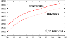
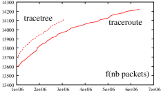
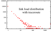
  $x$ = # rounds; $y$ = # ip   $x$ = # packets; $y$ = # ip   $x$ = # times probed; $y$ = # links

Figure 3: Comparison between traceroute and tracetree. Left and center: number of distinct ip addresses viewed since the beginning with a traceroute measurement (plain lines) and a tracetree measurement simulated from it (dotted lines); left: as a function of the number of rounds; center: as a function of the number of packets sent. To improve readability, we cut the part of the plots corresponding to the $20$ first rounds and to the $10^{6}$ first packets, respectively. Right: typical link load distribution with a traceroute ego-centered measurement. For each value $x$ on the horizontal axis, we give the number of links which are discovered $x$ times during a traceroute ego-centered measurement with 3 000 destinations (base value).

We also considered other observables (like the number of stars seen at each round, and the number of packets received after the timeout), for measurements obtained from various monitors and towards various destinations; in all cases, the conclusion was the same: the base parameters proposed above meet our requirements.

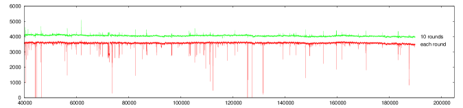
Figure 4: Bottom: number of distinct ip addresses observed during each round of measurement. Top: number of distinct ip addresses observed during series of ten consecutive rounds.

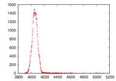
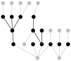
  $x$ = # ip ; $y$ = # series     $x$ = components size; $y$ = # components

Figure 5: Left: Distribution of the values of the upper plot in Figure 4. Center: typical islands of appearing nodes. Each node is an ip address; the black ones are the ones observed during the second half of the measurement only, the others being already present in the first half. The square nodes were present in all the ($2\,200$) rounds of measurement. Links are directed from bottom to top, i.e. from the monitor to destinations. The number of rounds necessary to discover all $13$ new nodes in the left drawing was $669$ rounds ($1\,306$ to $1\,974$), but only $2$ rounds ($2\,021$ and $2\,022$) were sufficient for the $9$ right ones. Notice that $7$ connected components of new nodes are displayed: $4$ of size $1$, $1$ of size $4$, $1$ of size $5$, and $1$ of size $9$. Right: distribution of new node component sizes. For each possible size $x$ (horizontal axis), the number of connected components of new nodes of size $x$ is given.

3.3 Comparison with traceroute.

As explained in Section 2.1, a key goal of our tracetree measurement tool is to perform significantly better than direct use of traceroute in our context. To evaluate this, we compare the difference in the obtained information with traceroute and tracetree, as well as the load they induce on the network (Figure 3, left and center). First notice that the plot as a function of the number of rounds with traceroute is higher than the one with tracetree, as expected: any traceroute round gathers slightly more data than the corresponding tracetree round (below $1\,\%$, here). It is however much more interesting to compare them in terms of the number of packets sent (reflecting the load induced on the network and our ability to increase the measurement frequency). The plots show that, to this regard, tracetree is much more efficient than direct traceroute measurements: here, tracetree reaches $14\,100$ distinct ip addresses with around $3$ millions packets, while traceroute needs around $4.5$ millions packets.

Recall moreover that the load induced by tracetree is balanced among links, which is not the case for traceroute, see Figure 3 (right). We can see that some links are probed a very high number of times at each round (typically up to $3\,000$ times if we use $3\,000$ destinations). See [12, 11, 10] for detailed studies of such effects.

Finally, in addition to the key advantage of providing homogeneous tree ego-centered views of the topology, the tracetree tool also is much more efficient than traceroute in terms of the number of packets sent, thus making it possible to repeatedly run it in radar measurements with a reasonable network cost.

4 Towards event detection.

One key interest of our measurements is that they make it possible to observe the dynamics of the ip internet topology from an ego-centered perspective, at a time scale of a few minutes only. In particular, detecting events in this dynamics, i.e. major changes in the topology, is very appealing from a security and modeling point of view.

A most natural direction to try and detect events is to observe the number of distinct ip addresses seen at each round, as plotted in Figure 4. Clear events indeed appear in such plots, under the form of downward peaks. However, this provides little information, if any: these peaks may be caused by temporary partial or total connectivity losses at the monitor (or close to it), not by important events at the internet level. On the other hand, one may notice that no significant upward peak appears in this plot. Notice that this is a non-trivial fact: from a topological point of view, such peaks would be possible; the fact that they do not occur reflects non-trivial properties of the topology and its dynamics, which we leave for further study.

Interestingly, the plot of the number of distinct ip addresses seen during ten consecutive rounds, Figure 4, has very different characteristics. It exhibits upward peaks (the distribution of observed values, presented in Figure 5, left, confirms that these peaks are statistically significant outliers). These peaks reveal important changes in the ip addresses observed in consecutive rounds, and thus important routing changes: though the number of observed ip addresses is roughly the same before and after these events, the ego-centered views have changed.

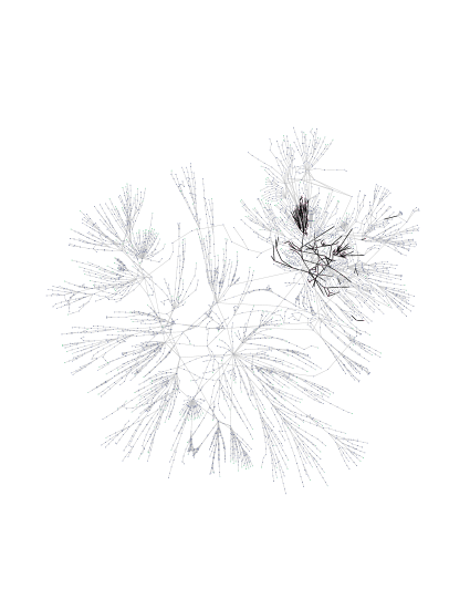
Figure 6: Representation of the event at round 106231 in Figure 4: the graph is obtained by merging 100 rounds before the event together with a single round after the event. Edges in bold black are edges that were seen in the round after the event but not in the 100 rounds before.

To illustrate this, we present in Figure 6 a graph obtained by merging ego-centered views measured before and after such an upward peak. We can clearly see that this peak corresponds to a large number of new edges appearing in a specific part of the network, confirming the occurrence of a significant event.

Another approach consists in detecting events occurring during a measurement from round $i$ to round $j$ by comparing it to the measurement from round $i-k$ to round $i$, which serves as a reference: we consider the ip addresses seen during the period of interest which were not observed in the reference period. We call these ip addresses the new addresses. Our observations show that it is natural to observe such new addresses during any measurement. However, one may expect that events of interest will lead to the appearance of connected groups of such addresses; we therefore propose to compute the connected components composed of new addresses  as a way to observe these events.

We display such components in Figure 5 (center), together with their neighborhood. This figure shows clearly that, in some cases, the observed components are non-trivial islands of newly observed nodes, revealing local events in the network. Figure 5 (right) however shows that such non-trivial islands are quite rare: most connected components of new nodes are very small, often reduced to a single node ($949$ over a total of $1\,457$ components, in our example). Despite this, some large components appear (the largest one in our example has size $17$, and $15$ components have size at least $10$), thus revealing underlying events of interest.

Another important characteristic of connected components of new addresses is the number of rounds needed to discover all their nodes, defined as the round number at which their last node was discovered minus the round number at which their first node was, plus one. Indeed, short discovery times indicate that all the new nodes under concern probably appeared because of a same event. Large times, instead, show that several events (located close to each other in the network) occurred. The examples in Figure 5 (center) show that both cases occur.

The distribution of the number of rounds needed to discover each component of new nodes (not represented here) is very heterogeneous, with many components discovered very rapidly and others much more slowly. This gives little information, however, as the discovery time may depend strongly on the component size. Studying the correlations between the two (not represented here) confirms this, but it also shows that some large connected components are discovered very rapidly.

The two approaches we described point out specific moments at which events occurred; one may then observe the data more closely, in order to investigate the nature of these events. We leave this for further research.

5 Conclusion and perspectives.

In this paper, we propose, implement, and illustrate a new measurement approach which makes it possible to study the dynamics of ip-level internet topology at a time scale of a few minutes. We provide a rich dataset consisting in radar measurements from more than one hundred monitors towards thousands of destinations, conducted for several weeks in continuous.

The most important direction for further research is of course the analysis of collected data. A particularly appealing goal is the detection of events in the dynamics of the observed topology; this raises difficult fundamental questions, such as the characterization of normal dynamics, or the identification of relevant time scales for the observation.

Other promising directions include visualizing the observed dynamics, and conducting more radar measurements to gain a deeper insight (for instance, one could conduct simultaneous measurements from several monitors to observe the dynamics from different viewpoints).

Acknowledgments. We warmly thank the PhD students and other colleagues of the LIP6, in particular Guillaume Valadon, Renata Teixeira, and Brice Augustin who provided great insight during this work. Likewise, we thank Benoît Donnet, who helped much with the references and also provided useful comments. Many interesting discussions within the METROSEC project [1] also played a key role in our work.

We also thank all the people who provided monitors to us, in particular the PlanetLab staff [25], Frédéric Aidouni, Julien Aussibal, Prof. Hiroshi Esaki (WIDE), Jean-Charles de Longueville (Hellea) and Sébastien Wacquiez (Enix); no such work would be possible without their help.

This work was funded in part by the METROSEC and AGRI projects.

References

- [1] Metrosec project. http://www2.laas.fr/METROSEC/.
- [2] Supplementary material (programs and data). http://www-rp.lip6.fr/~latapy/Radar/.
- [3] traceroute@home project. http://trhome.sourceforge.net/.
- [4] D. Achlioptas, A. Clauset, D. Kempe, and C. Moore. On the bias of traceroute sampling. In Proc. ACM STOC, 2005.
- [5] B. Augustin, T. Friedman, and R. Teixeira. Multipath Tracing with Paris Traceroute. In Proc. Workshop on End-to-End Monitoring, E2EMON, May 2007.
- [6] P. Barford, A. Bestavros, J. Byers, and M. Crovella. On the marginal utility of network topology measurements. In Proc. ACM SIGCOMM Internet Measurement Workshop (IMW), Nov. 2001.
- [7] S. Branigan, H. Burch, W. R. Cheswick, and F. Wojcik. What can you do with traceroute? IEEE Internet Computing, 5(5), Sept./Oct. 2001.
- [8] Q. Chen, H. Chang, R. Govindan, S. Jamin, S. Shenker, and W. Willinger. The origin of power laws in internet topologies revisited. In Proc. IEEE INFOCOM, Jun. 2002.
- [9] L. Dall’Asta, J. I. Alvarez-Hamelin, A. Barrat, A. Vázquez, and A. Vespignani. Exploring networks with traceroute-like probes: Theory and simulations. Theor. Comput. Sci., 355(1):6–24, 2006.
- [10] B. Donnet, P. Raoult, and T. Friedman. Efficient route tracing from a single source. cs.NI 0605133, arXiv, May 2006.
- [11] B. Donnet, P. Raoult, T. Friedman, and M. Crovella. Efficient algorithms for large-scale topology discovery. In Proc. ACM SIGMETRICS, Jun. 2005.
- [12] B. Donnet, P. Raoult, T. Friedman, and M. Crovella. Deployment of an algorithm for large-scale topology discovery. IEEE Journal on Selected Areas in Communications, Sampling the Internet: Techniques and Applications, 24(12):2210–2220, Dec. 2006.
- [13] M. Faloutsos, P. Faloutsos, and C. Faloutsos. On power-law relationships of the internet topology. In Proc. ACM SIGCOMM, 1999.
- [14] F. Georgatos, F. Gruber, D. Karrenberg, M. Santcroos, A. Susanj, H. Uijterwaal, and R. Wilhelm. Providing active measurements as a regular service for ISPs. In Proc. of Passive and Active Measurement Workshop, 2001. See also the RIPE NCC TTM service: http://www.ripe.net/test-traffic/.
- [15] R. Govindan and V. Paxson. Estimating router ICMP generation delays. In Proc. of Passive and Active Measurement Workshop, March 2002.
- [16] R. Govindan and H. Tangmunarunkit. Heuristics for internet map discovery. In Proc. IEEE INFOCOM, Mar. 2000.
- [17] J. L. Guillaume and M. Latapy. Relevance of massively distributed explorations of the internet topology: Simulation results. In Proc. IEEE INFOCOM, Mar. 2005.
- [18] B. Huffaker, D. Plummer, D. Moore, and k. claffy. Topology discovery by active probing. In Proc. Symposium on Applications and the Internet, Jan. 2002.
- [19] A. Lakhina, J. Byers, M. Crovella, and P. Xie. Sampling biases in IP topology measurements. In Proc. IEEE INFOCOM, Apr. 2003.
- [20] M. Luckie. IPv6 scamper, 2005. WAND Network Research Group. See http://www.wand.net.nz/~mjl12/ipv6-scamper/.
- [21] A. McGregor, H.-W. Braun, and J. Brown. The NLANR network analysis infrastructure. IEEE Communications Mag., 38(5):122–128, May 2000. See also the NLANR AMP project: http://watt.nlanr.net/.
- [22] T. Moors. Streamlining traceroute by estimating path lengths. In Proc. IEEE International Workshop on IP Operations and Management (IPOM), Oct. 2004.
- [23] R. Oliveira, B. Zhang, and L. Zhang. Observing the evolution of internet AS topology. In Proc. ACM SIGCOMM, 2007.
- [24] J.-J. Pansiot. Local and dynamic analysis of internet multicast router topology. Annales des télécommunications, 62:408–425, 2007.
- [25] PlanetLab Consortium. PlanetLab project, 2002. See http://www.planet-lab.org.
- [26] Y. Shavitt and E. Shir. DIMES: Let the internet measure itself. ACM SIGCOMM Computer Communication Review, 35(5):71 – 74, October 2005.
- [27] N. Spring, D. Wetherall, and T. Anderson. Scriptroute: A public internet measurement facility. In Proc. 4th USENIX Symposium on Internet Technologies and Systems, 2002. see also http://www.cs.washington.edu/research/networking/scriptroute/.
- [28] F. Viger, B. Augustin, X. Cuvellier, C. Magnien, M. Latapy, T. Friedman, and R. Teixeira. Detection, understanding, and prevention of traceroute measurement artifacts. Computer Networks, 52, 2008.
- [29] D. G. Waddington, F. Chang, R. Viswanathan, and B. Yao. Topology discovery for public IPv6 networks. ACM SIGCOMM Computer Communication Review, 33(3):59–68, Jul. 2003.