arXiv:0807.1597 [hep-lat]

Stochastic quantization at finite chemical potential

Abstract

A nonperturbative lattice study of QCD at finite chemical potential is complicated due to the complex fermion determinant and the sign problem. Here we apply the method of stochastic quantization and complex Langevin dynamics to this problem. We present results for U(1) and SU(3) one link models and QCD at finite chemical potential using the hopping expansion. The phase of the determinant is studied in detail. Even in the region where the sign problem is severe, we find excellent agreement between the Langevin results and exact expressions, if available. We give a partial understanding of this in terms of classical flow diagrams and eigenvalues of the Fokker-Planck equation.

1 Introduction

A nonperturbative understanding of QCD at nonzero baryon density remains one of the outstanding problems in the theory of strong interactions. Besides the theoretical challenge, there is a clear phenomenological interest in pursuing these studies, due to the ongoing developments in heavy ion collision experiments, at RHIC, LHC and the planned FAIR facility at GSI.

The standard nonperturbative tool to study quarks and gluons, lattice QCD, cannot be applied in a straightforward manner, because the complexity of the fermion determinant prohibits the use of approaches based on importance sampling. This is commonly referred to as the sign problem. Since the start of the millenium a number of new methods has been devised. These include reweighting [1, 2, 3, 4], Taylor series expansion in $\mu/T$ [5, 6, 7, 8], imaginary chemical potential and analytical continuation [9, 10, 11, 12], and the use of the canonical ensemble [13, 14] and the density of states [15]. Except for the last two, these approaches are approximate by construction and aimed at describing the QCD phase diagram in the region of small chemical potential and temperatures around the crossover between the confined and the deconfined phase. In this paper we discuss an approach which is manifestly independent of those listed above: stochastic quantization and complex Langevin dynamics. How well this method will work is not known a priori. However, one of the findings of our study is that excellent agreement is found in the case of simple models, where comparison with results obtained differently is available. In particular we find that the range of applicability is not restricted to small chemical potential and, importantly, does not depend on the severity of the sign problem. The first results we present for lattice QCD at nonzero density are encouraging, although a systematic analysis has not yet been performed.

This paper is organized as follows. In the following section we briefly describe the idea behind stochastic quantization and the necessity to use complex Langevin dynamics in the case of nonzero chemical potential. In Secs. 3 and 4 we apply this technique to U(1) and SU(3) one link models. In both cases a comparison with exact results can be made. We study the phase of the determinant in detail. In the case of the U(1) model, we employ the possibility to analyse classical flow diagrams and the Fokker-Planck equation to gain further understanding of the results. In Sec. 5 we turn to QCD, using the full gauge dynamics but treating the fermion determinant in the hopping expansion. Our findings and outlook to the future are summarized in Sec. 6. The Appendix contains a brief discussion of the Fokker-Planck equation in Minkowski time for the one link U(1) model.

2 Stochastic quantization and complex Langevin dynamics

The main idea of stochastic quantization [16, 17] is that expectation values are obtained as equilibrium values of a stochastic process. To implement this, the system evolves in a fictitious time direction $\theta$, subject to stochastic noise, i.e.  it evolves according to Langevin dynamics. Consider for the moment a real scalar field $\phi(x)$ in $d$ dimensions with a real euclidean action $S$. The Langevin equation reads

$$\frac{\partial\phi(x,\theta)}{\partial\theta}=-\frac{\delta S[\phi]}{\delta\phi(x,\theta)}+\eta(x,\theta),$$ (2.1)

where the noise satisfies

$$\langle\eta(x,\theta)\rangle=0,\;\;\;\;\;\;\;\;\langle\eta(x,\theta)\eta(x^{\prime},\theta^{\prime})\rangle=2\delta(x-x^{\prime})\delta(\theta-\theta^{\prime}).$$ (2.2)

By equating expectation values, defined as

$$\langle O[\phi(x,\theta)]\rangle_{\eta}=\int D\phi\,P[\phi,\theta]O[\phi(x)],$$ (2.3)

where $O$ is an arbitrary operator and the brackets on the left-hand side denote a noise average, it can be shown that the probability distribution $P[\phi,\theta]$ satisfies the Fokker-Planck equation

$$\frac{\partial P(\phi,\theta)}{\partial\theta}=\int d^{d}x\,\frac{\delta}{\delta\phi(x,\theta)}\left(\frac{\delta}{\delta\phi(x,\theta)}+\frac{\delta S[\phi]}{\delta\phi(x,\theta)}\right)P[\phi,\theta].$$ (2.4)

In the case of a real action $S$, the stationary solution of the Fokker-Planck equation, $P[\phi]\sim\exp\left(-S[\phi]\right)$, will be reached in the large time limit $\theta\to\infty$, ensuring convergence of the Langevin dynamics to the correct equilibrium distribution. When the action is complex, as is the case in QCD at finite chemical potential, the situation is not so easy. It is still possible to consider Langevin dynamics based on Eq. (2.1) [18, 19, 20, 21]. However, due to the complex force on the right-hand side, fields will now be complex as well: $\phi\to\mbox{Re\,}\phi+i\mbox{Im\,}\phi$. As a result, proofs of the convergence towards the (now complex) weight $e^{-S}$ are problematic.

In the past, complex Langevin dynamics has been applied to effective three-dimensional spin models with complex actions, related to lattice QCD at finite $\mu$ in the limit of strong coupling and large fermion mass [22, 23, 24] (for applications to other models, see e.g. Ref. [25]). Our work has also partly been inspired by the recent application of stochastic quantization to solve nonequilibrium quantum field dynamics [26, 27, 28]. In that case the situation is even more severe. Nevertheless, numerical convergence towards a solution can be obtained under certain conditions, both for simple models and four-dimensional field theories. For an illustration we present some original results in the appendix.

Here we consider models with a partition function whose form is motivated by or derived from QCD at finite chemical potential. The QCD partition function reads

$$Z=\int DU\,e^{-S_{B}}\det M,$$ (2.5)

where $S_{B}(U)$ is the bosonic action depending on the gauge links $U$ and $\det M$ is the complex fermion determinant, satisfying

$$\det M(\mu)=[\det M(-\mu)]^{*}.$$ (2.6)

Specifically, for Wilson fermions the fermion matrix has the schematic form

$$M=1-\kappa\sum_{i=1}^{3}\left(\Gamma_{+i}U_{x,i}T_{i}+\Gamma_{-i}U_{x,i}^{\dagger}T_{-i}\right)-\kappa\left(e^{\mu}\Gamma_{+4}U_{x,4}T_{4}+e^{-\mu}\Gamma_{-4}U_{x,4}^{\dagger}T_{-4}\right).$$ (2.7)

Here $T$ are lattice translations, $\Gamma_{\pm\mu}=1\!\!1\pm\gamma_{\mu}$, and $\kappa$ is the hopping parameter. Chemical potential is introduced by multiplying the temporal links in the forward (backward) direction with $e^{\mu}$ ($e^{-\mu}$) [29]. We use Eq. (2.7) as a guidance to construct the U(1) and SU(3) one link models considered next.

3 One link U(1) model

3.1 Complex Langevin dynamics

We consider a one link model with one degree of freedom, written as $U=e^{ix}$. The partition function is written suggestively as

$$Z=\int dU\,e^{-S_{B}}\det M=\int_{-\pi}^{\pi}\frac{dx}{2\pi}\,e^{-S_{B}}\det M,$$ (3.1)

where the “bosonic” part of the action reads

$$S_{B}(x)=-\frac{\beta}{2}\left(U+U^{-1}\right)=-\beta\cos x,$$ (3.2)

while the “determinant” is constructed by multiplying the forward (backward) link with $e^{\mu}$ ($e^{-\mu}$),

$$\det M=1+\frac{1}{2}\kappa\left[e^{\mu}U+e^{-\mu}U^{-1}\right]=1+\kappa\cos(x-i\mu).$$ (3.3)

Due to the chemical potential, the determinant is complex and has the same property as the fermion determinant in QCD, i.e. $\det M(\mu)=[\det M(-\mu)]^{*}$. For an imaginary chemical potential $\mu=i\mu_{I}$, the determinant is real, as is the case in QCD.

Observables are defined as

$$\langle O(x)\rangle=\frac{1}{Z}\int_{-\pi}^{\pi}\frac{dx}{2\pi}\,e^{-S_{B}}\det M\,O(x).$$ (3.4)

In this model most expectation values can be evaluated analytically. We consider here the following observables:

• Polyakov loop:

  $$\langle U\rangle=\langle e^{ix}\rangle=\frac{1}{Z}\left[I_{1}(\beta)+\kappa I_{1}^{\prime}(\beta)\cosh\mu-\kappa I_{1}(\beta)/\beta\sinh\mu\right],$$ (3.5)

  where the partition function equals

  $$Z=I_{0}(\beta)+\kappa I_{1}(\beta)\cosh\mu,$$ (3.6)

  and $I_{n}(\beta)$ are the modified Bessel functions of the first kind.

• Conjugate Polyakov loop:

  $$\langle U^{-1}\rangle=\langle e^{-ix}\rangle=\langle e^{ix}\rangle\bigg{|}_{\mu\to-\mu}.$$ (3.7)

  At finite chemical potential, $\langle U\rangle$ and $\langle U^{-1}\rangle$ are both real, but different.

• Plaquette:

  $$\langle\cos x\rangle=\frac{\partial}{\partial\beta}\ln Z=\frac{1}{Z}\left[I_{1}(\beta)+\kappa I_{1}^{\prime}(\beta)\cosh\mu\right].$$ (3.8)

  Note that $\langle\cos x\rangle=\frac{1}{2}\langle e^{ix}+e^{-ix}\rangle$.

• Density:

  $$\langle n\rangle=\frac{\partial}{\partial\mu}\ln Z=\left\langle\frac{i\kappa\sin(x-i\mu)}{1+\kappa\cos(x-i\mu)}\right\rangle=\frac{1}{Z}\kappa I_{1}(\beta)\sinh\mu.$$ (3.9)

  At small chemical potential $\langle n\rangle$ increases linearly with $\mu$, while at large chemical potential $\langle n\rangle\to 1$ exponentially fast.

We now aim to estimate these observables using numerical techniques. Due to the complexity of the determinant, they cannot be estimated using methods based on importance sampling. Instead, we attempt to obtain expectation values using stochastic quantization.

At nonzero chemical potential, the action is complex and it becomes necessary to consider complex Langevin dynamics. We write therefore $x\to z=x+iy$, and consider the following complex Langevin equations

$$x_{n+1}= x_{n}+\epsilon K_{x}(x_{n},y_{n})+\sqrt{\epsilon}\eta_{n},$$ (3.10)

$$y_{n+1}= y_{n}+\epsilon K_{y}(x_{n},y_{n}).$$ (3.11)

Here we have discretized Langevin time as $\theta=n\epsilon$, and the noise satisfies

$$\langle\eta_{n}\rangle=0,\;\;\;\;\;\;\;\;\langle\eta_{n}\eta_{n^{\prime}}\rangle=2\delta_{nn^{\prime}}.$$ (3.12)

The drift terms are given by

$$K_{x}=-\mbox{Re\,}\frac{\partial S_{\rm eff}}{\partial x}\Bigg{|}_{x\to x+iy},\;\;\;\;\;\;\;\;K_{y}=-\mbox{Im\,}\frac{\partial S_{\rm eff}}{\partial x}\Bigg{|}_{x\to x+iy},$$ (3.13)

where the effective action reads

$$S_{\rm eff}=S_{B}-\ln\det M=-\beta\cos x-\ln\left[1+\kappa\cos(x-i\mu)\right].$$ (3.14)

Explicitly, the drift terms are

$$K_{x}= -\sin x\left[\beta\cosh y+\kappa\frac{\cosh(y-\mu)+\kappa\cos x}{D(x)}\right],$$ (3.15)

$$K_{y}= -\beta\cos x\sinh y-\kappa\sinh(y-\mu)\frac{\cos x+\kappa\cosh(y-\mu)}{D(x)},$$ (3.16)

where

$$D(x)=\left[1+\kappa\cos x\cosh(y-\mu)\right]^{2}+\left[\kappa\sin x\sinh(y-\mu)\right]^{2}.$$ (3.17)

Occasionally we will also consider this model by expanding in small $\kappa$, the hopping expansion, and take

$$S_{\rm eff}=-\beta\cos x-\kappa\cos(x-i\mu)\;\;\;\;\;\;\;\;\mbox{(hopping expansion)}.$$ (3.18)

This limit is motivated by the model of Heavy Dense Matter used in Ref. [36]. A direct application of our method to QCD in the hopping expansion is presented in Sec. 5.

In order to compute expectation values, also the observables have to be complexified. For example, after complexification $x\to z=x+iy$, the plaquette reads

$$\cos x\to\cos(x+iy)=\cos x\cosh y-i\sin x\sinh y.$$ (3.19)

All operators we consider are now complex, with the real (imaginary) part being even (odd) under $x\to-x$.

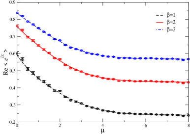
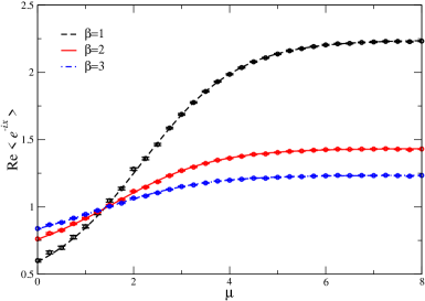
Figure 1: Real part of the Polyakov loop $\langle e^{ix}\rangle$ (left) and the conjugate Polyakov loop $\langle e^{-ix}\rangle$ (right) as a function of $\mu$ for three values of $\beta$ at fixed $\kappa=1/2$. The lines are the analytical results, the symbols are obtained with complex Langevin dynamics.

The Langevin dynamics can be solved numerically. In Fig. 1 the real parts of the Polyakov loop and the conjugate Polyakov loop are shown as a function of $\mu$ for three values of $\beta$ at fixed $\kappa=1/2$. In Fig. 2 (left) the density is shown. The lines are the exact analytical results. The symbols are obtained with the stochastic quantization. We observe excellent agreement between the analytical and numerical results. For the results shown here and below, we have used Langevin stepsize $\epsilon=5\times 10^{-5}$ and $5\times 10^{7}$ time steps. Errors are estimated with the jackknife procedure. The imaginary part of all observables shown here is consistent with zero within the error in the Langevin dynamics. This can be understood from the symmetries of the drift terms and the complexified operators, since the drift terms behave under $x\to-x$ as

$$K_{x}(-x,y;\mu)=-K_{x}(x,y;\mu),\;\;\;\;\;\;\;\;K_{y}(-x,y;\mu)=K_{y}(x,y;\mu),$$ (3.20)

while the imaginary parts are odd. Therefore, after averaging over the Langevin trajectory the expectation value is expected to reach zero within the error, which is what we observe. As an aside, we note that the symmetry of the drift terms under $y\to-y$,

$$K_{x}(x,-y;-\mu)=K_{x}(x,y;\mu),\;\;\;\;\;\;\;\;K_{y}(x,-y;-\mu)=-K_{y}(x,y;\mu),$$ (3.21)

relates positive and negative chemical potential.

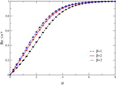
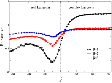
Figure 2: Left: Real part of the density $\langle n\rangle$. Right: Real part of the plaquette $\langle\cos x\rangle$ versus $\mu^{2}$. Results at positive (negative) $\mu^{2}$ have been obtained with complex (real) Langevin evolution.

At imaginary chemical potential $\mu=i\mu_{I}$ the determinant is real, so that the complexification of the Langevin dynamics is not necessary. We demonstrate the smooth connection for results obtained at imaginary $\mu$ using real Langevin dynamics and results obtained at real $\mu$ using complex Langevin dynamics for the expectation value of the plaquette $\langle\cos x\rangle$ in Fig. 2 (right). Since the plaquette is even under $\mu\to-\mu$, we show the result as a function of $\mu^{2}$, so that the left side of the plot corresponds to imaginary chemical potential, while the right side corresponds to real chemical potential. On both sides excellent agreement with the analytical expression can be observed. We also note that the errors are comparable on both sides.

3.2 Phase of the determinant

At finite chemical potential the determinant is complex and can be written as

$$\det M=|\det M|e^{i\phi}.$$ (3.22)

In order to assess the severity of the sign problem, we consider the phase of the determinant and study the behaviour of $e^{i\phi}$. An observable often used for this purpose [38, 39] is

$$\langle e^{2i\phi}\rangle=\left\langle\frac{\det M(\mu)}{\det M(\mu)^{*}}\right\rangle=\left\langle\frac{\det M(\mu)}{\det M(-\mu)}\right\rangle,$$ (3.23)

where we used Eq. (2.6). At zero chemical potential the ratio equals one, while at large $\mu$ one finds in this model that

$$\lim_{\mu\to\infty}\langle e^{2i\phi}\rangle=\frac{I_{3}(\beta)}{I_{1}(\beta)}+{\cal O}(e^{-\mu}),$$ (3.24)

for nonzero $\beta$. In expressing Eq. (3.23) as the expectation value obtained from the complex Langevin process, complex conjugation has to be performed after the complexification of the variables, as discussed above. In that case $\det M(\mu)^{*}$ as a complex number is not the complex conjugate of $\det M(\mu)$. To avoid confusion we write ${\det M(-\mu)}$ in all relevant expressions. Notice that this implies that $\phi$ itself is also complex.

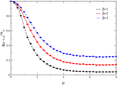
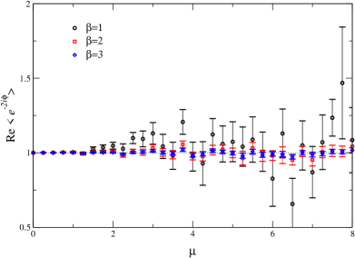
Figure 3: Left: Real part of $\langle e^{2i\phi}\rangle=\langle\det M(\mu)/\det M(-\mu)\rangle$. Right: Real part of $\langle e^{-2i\phi}\rangle=\langle\det M(-\mu)/\det M(\mu)\rangle=Z(-\mu)/Z(\mu)$.

In Fig. 3 (left) we show the real part of this observable as a function of $\mu$. The imaginary part is again zero analytically and zero within the error in the Langevin process. The lines are obtained by numerical integration of the observable with the complex weight, while the symbols are again obtained from Langevin dynamics. We note again excellent agreement between the semi-analytical and the stochastic results. In particular, there seems to be no problem in accessing the region with larger $\mu$ where the average phase factor becomes very small. The numerical error is under control in the entire range. We find therefore that the sign problem does not appear to be a problem for this method in this model.

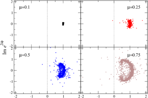
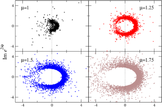
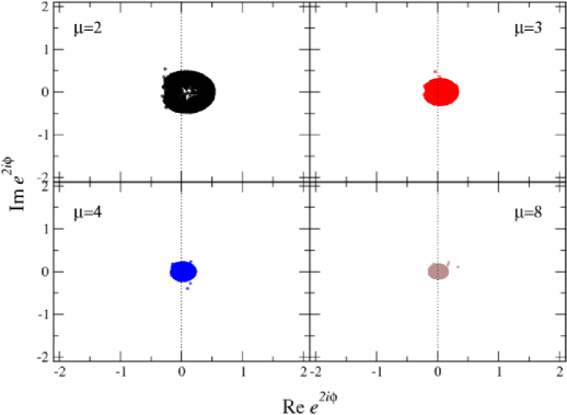
Figure 4: Scatter plot of $e^{2i\phi}=\det M(\mu)/\det M(-\mu)$ during the Langevin evolution for various values of $\mu$ at $\beta=1$, $\kappa=1/2$. Note the different scale in the middle box.

In contrast to what could be inferred from the result above, expectation values of $e^{i\phi}$ are not phase factors, due to the complexity of the action. This can be seen by considering

$$\langle e^{-2i\phi}\rangle=\left\langle\frac{\det M(-\mu)}{\det M(\mu)}\right\rangle=\frac{Z(-\mu)}{Z(\mu)}=1,$$ (3.25)

where the second and third equality follow from the cancelation of det $M(\mu)$ in the definition of the expectation value and from $Z$ being even in $\mu$. We have also computed this observable using Langevin dynamics and the result is shown in Fig. 3 (right). For the Langevin parameters used here, we observe that the numerical estimate is consistent with 1, but with quite large errors when $\mu$ increases at small values of $\beta$. We have found that increasing the Langevin time reduces the uncertainty. We conclude that at large chemical potential this ratio of determinants is the most sensitive and slowest converging observable we considered.

We observed above that the average phase factor becomes very small at large $\mu$ but that this does not manifest itself in all but one observable we consider. Insight into this feature can be gained by studying scatter plots of the phase factor during the Langevin process. In Fig. 4 we show the behaviour of $e^{2i\phi}$ during the Langevin evolution in the two-dimensional plane spanned by $\mbox{Re\,}e^{2i\phi}$ and $\mbox{Im\,}e^{2i\phi}$. At zero chemical potential, $\mbox{Re\,}e^{2i\phi}=1$ and $\mbox{Im\,}e^{2i\phi}=0$ during the entire evolution. For increasing $\mu$ one finds more and more deviations from this, with an interesting structure at intermediate values of $\mu$. Note that the resulting distribution is approximately invariant under reflection in $\mbox{Im\,}e^{2i\phi}\to-\mbox{Im\,}e^{2i\phi}$, ensuring that the imaginary part of the expectation value $\langle e^{2i\phi}\rangle$ vanishes within the error. Due to the wide distribution, the horizontal and vertical scales in the middle section of Fig. 4 are much larger than in the top and bottom part. However, the average phase factor remains well defined for all values of $\mu$, as can be seen in Fig. 3. At large $\mu$, the average phase factor becomes very small. However, the distribution is very narrow, see Fig. 4 (bottom). Therefore, although the average is close to zero, the error in the Langevin dynamics is very well under control.

3.3 Fixed points and classical flow

The excellent results obtained above can partly be motivated by the structure of the dynamics in the classical limit, i.e. in absence of the noise. As we demonstrate below, the classical flow and fixed point structure is easy to understand when $\mu=0$ and, most importantly, does not change qualitatively in the presence of nonzero chemical potential.

Classical fixed points are determined by the extrema of the classical (effective) action, i.e. by putting $K_{x}=K_{y}=0$. We first consider the “bosonic” model and take $\kappa=0$. The drift terms are

$$K_{x}(x,y)=-\beta\sin x\cosh y,\;\;\;\;\;\;\;\;K_{y}(x,y)=-\beta\cos x\sinh y.$$ (3.26)

We see that there is one stable fixed point at $(x,y)=(0,0)$ and one unstable fixed point at $(\pi,0)$. Moreover, the classical flow equation, $dz/d\theta=-\beta\sin z$, can be solved analytically, with the solution

$$\tan\frac{z(\theta)}{2}=e^{-\beta(\theta-\theta_{0})}\tan\frac{z(0)}{2},$$ (3.27)

where $z(0)$ is the initial value at $\theta=\theta_{0}$. We find therefore that the stable fixed point is reached for all $z(0)$, except when $x(0)=\pi$. On this line the solution reads

$$\tanh\frac{y(\theta)}{2}=e^{\beta(\theta-\theta_{0})}\tanh\frac{y(0)}{2},$$ (3.28)

and the flow diverges to $y\to\pm\infty$, except when starting precisely on the unstable fixed point $(\pi,0)$. Note, however, that the noise in the $x$ direction will kick the dynamics of the unstable trajectories.

We now include the determinant, starting with the hopping expansion (3.18). Putting $K_{x}=K_{y}=0$ yields again one stable fixed point at $(x,y)=(0,y_{*})$ and one unstable fixed point at $(\pi,y_{*})$, where

$$\tanh y_{*}=\frac{\kappa\sinh\mu}{\beta+\kappa\cosh\mu}.$$ (3.29)

Note that in the strong coupling limit $y_{*}=\mu$. We find therefore a simple modification of the bosonic model: in response to the chemical potential the two fixed points move in the vertical $y$ direction, but not in the $x$ direction.

We continue with the full determinant included. Consider the case with $\mu=0$ first, where real dynamics can be considered. Again we find the stable fixed point at $x=0$ and the unstable fixed point at $x=\pi$. Provided that

$$\gamma\equiv\left(\frac{1}{\beta}+\frac{1}{\kappa}\right)>1,$$ (3.30)

there are no additional fixed points. In order to satisfy this condition, we take $\kappa<1$ throughout. Using complex dynamics, while keeping $\mu=0$, we find that the stable fixed point at $(x,y)=(0,0)$ remains, but that there are now three unstable fixed points at $x=\pi$, given by $(\pi,0)$ and $(\pi,\pm y_{*})$, with $\cosh y_{*}=\gamma$. Interestingly, the fixed-point structure is therefore different for real and complex flow.

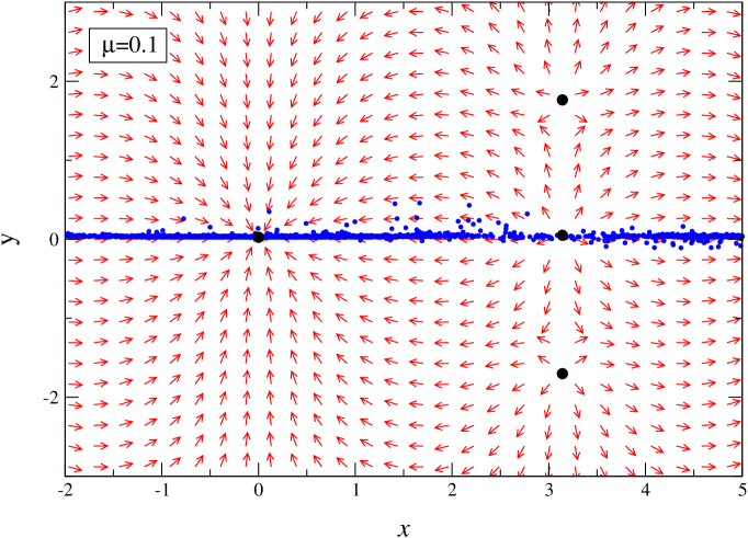
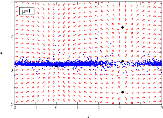
Figure 5: Classical flow diagram in the $x-y$ plane for $\beta=1$, $\kappa=1/2$, $\mu=0.1$ (top) and $\mu=1$ (bottom). The big dots indicate the fixed points at $x=0$ and $\pi$. The small circles indicate a trajectory during the Langevin evolution, each dot separated from the previous one by 500 steps. Note the periodicity $x\to x+2\pi$.

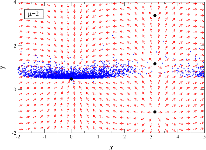
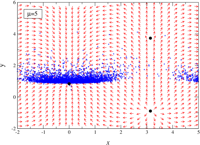
Figure 6: As in the previous figure, with $\mu=2$ (top) and $\mu=5$ (bottom).

Finally, we come to the full determinant at finite chemical potential. In this case the fixed points can only be determined numerically. We find a stable fixed point at $(x,y)=(0,y_{s})$ and unstable fixed points at $(x,y)=(\pi,y_{u})$. The $y$ coordinates of these fixed points are determined by

$$K_{y}\Big{|}_{x=0,\pi}=\mp\beta\sinh y\mp\frac{\kappa\sinh(y-\mu)}{1\pm\kappa\cosh(y-\mu)}=0,$$ (3.31)

where the upper (lower) sign applies to $y_{s}$ ($y_{u}$). At $x=0$ there is only one solution, while at $x=\pi$ we find numerically that there are three (unstable) solutions for small chemical potential, two for intermediate $\mu$ and only one for large $\mu$. Although the number of fixed points at $x=\pi$ depends on $\mu$, we find that they are always unstable such that this has no effect on the dynamics, which is attracted to the stable fixed point at $x=0$.

In Figs. 5 and 6 we show the classical flow diagrams in the $x-y$ plane. The direction of the arrows indicates $(K_{x},K_{y})$, evaluated at $(x,y)$. The lengths of the arrows are normalized for clarity. The fixed points are indicated with the larger black dots. In the bosonic model ($\kappa=0$), the analytical solution showed that the fixed point at $x=0$ is globally attractive, except when $x=\pi$. At nonzero $\kappa$ and $\mu$, the fixed point at $x=0$ appears to be globally attractive as well, except again for $x=\pi$. The small (blue) dots are part of a Langevin trajectory, each dot separated from the previous one by 500 steps. For vanishing $\mu$, the dynamics takes place in the $x$ direction only; for increasing $\mu$ it spreads more and more in the $y$ direction. An interesting asymmetry around the classical fixed point in the $y$ direction can be observed. However, the dynamics remains well contained in the $x-y$ plane.

We conclude therefore that the complex Langevin dynamics does not change qualitatively in the presence of a chemical potential, small or large. We take this as a strong indication that the method is insensitive to the sign problem.

3.4 Fokker-Planck equation

The microscopic dynamics of the Langevin equation,

$$\frac{\partial x}{\partial\theta}=-\frac{\partial S}{\partial x}+\eta,$$ (3.32)

where $\theta$ is the (continuous) Langevin time, can be translated into the dynamics of a distribution $P(x,\theta)$, via the relation

$$\langle O(x,\theta)\rangle_{\eta}=\int\frac{dx}{2\pi}P(x,\theta)O(x).$$ (3.33)

From the Langevin equation, it follows that $P(x,\theta)$ satisfies a Fokker-Planck equation,

$$\frac{\partial}{\partial\theta}P(x,\theta)=L_{\rm FP}^{c}P(x,\theta),$$ (3.34)

where $L_{\rm FP}^{c}$ is the complex Fokker-Planck operator

$$L_{\rm FP}^{c}=\frac{\partial}{\partial x}\left(\frac{\partial}{\partial x}+\frac{\partial S}{\partial x}\right).$$ (3.35)

The stationary solution of the Fokker-Planck equation is easily found by putting $L_{\rm FP}^{c}P(x)=0$ and is given by $P_{\rm st}(x)\sim\exp[-S(x)]$. In order to cast Eq. (3.34) as an eigenvalue problem, we write $P(x,\theta)=e^{-\lambda\theta}P^{(\lambda)}(x)$. The solution of the Fokker-Planck equation can then be written as

$$P(x,\theta)=\frac{e^{-S(x)}}{Z}+\sum_{\lambda}e^{-\lambda\theta}P^{(\lambda)}(x).$$ (3.36)

It is therefore interesting to study the properties of the Fokker-Planck equation and the nonzero eigenvalues $\lambda$.

In order to do so, we consider the model in the hopping expansion (3.18), with the action

$$S=-\beta\cos x-\kappa\cos(x-i\mu).$$ (3.37)

Explicitly, the Fokker-Planck equation then reads

$$\dot{P}(x,\theta)= P^{\prime\prime}(x,\theta)+\left[\beta\sin x+\kappa\sin(x-i\mu)\right]P^{\prime}(x,\theta)$$ (3.38)

$$+\left[\beta\cos x+\kappa\cos(x-i\mu)\right]P(x,\theta),$$

where primes/dots indicate $x$/$\theta$ derivatives. Using periodicity, $P(x+2\pi,\theta)=P(x,\theta)$, we decompose

$$P(x,\theta)=\sum_{n\in\mathbb{Z}}e^{-inx}P_{n}(\theta),\\ \;\;\;\;\;\;\;\;P_{n}(\theta)=\int_{-\pi}^{\pi}\frac{dx}{2\pi}\,e^{inx}P(x,\theta),$$ (3.39)

and we find

$$\dot{P}_{n}(\theta)=-n^{2}P_{n}(\theta)-nc_{+}P_{n+1}(\theta)+nc_{-}P_{n-1}(\theta),$$ (3.40)

with

$$c_{\pm}=\frac{1}{2}\left(\beta+\kappa e^{\pm\mu}\right).$$ (3.41)

We note that this equation is completely real, such that all $P_{n}(\theta)$’s are real. This is expected for the stationary solution, since from $S^{*}(x)=S(-x)$ it follows that $P^{*}_{\rm st}(x)=P_{\rm st}(-x)$ and therefore $P_{n,\rm st}^{*}=P_{n,\rm st}$. The numerical solution of Eq. (3.40) is shown in Fig. 7 for a number of modes $P_{n}(\theta)$ for $\mu=1$ (left) and 3 (right). The initial values $P_{n}(0)=1$ for all $n$. The number of modes is truncated, with $-50<n<50$. For large $\pm n$, $P_{n}(\theta)\to 0$ exponentially fast. The zero mode $P_{0}$ is $\theta$ independent and equal to 1 by construction. We have verified that the other modes converge to the values determined by the stationary solution $\sim e^{-S}$.

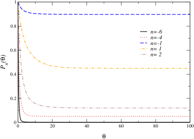
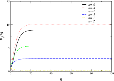
Figure 7: Solution of the complex Fokker-Planck equation: Langevin time dependence of the modes $P_{n}(\theta)$ for various values of $n$, with $\beta=1$, $\kappa=1/2$, and $\mu=1$ (left) and $\mu=3$ (right).

The convergence properties can be understood from the eigenvalues of the Fokker-Planck operator. Writing $P_{n}(\theta)=\exp(-\lambda\theta)P_{n}$ gives the eigenvalue equation

$$n^{2}P_{n}+nc_{+}P_{n+1}-nc_{-}P_{n-1}=\lambda P_{n}.$$ (3.42)

Since all $P_{n}$ are real, also all eigenvalues $\lambda$ are real. Although at first sight this may seem surprising, it is a consequence of the symmetry of the action and therefore it also holds in e.g. the full model.

The case $\lambda=0$ corresponds to the stationary solution. Here we consider $\lambda\neq 0$. First take $n=0$. It follows from Eq. (3.42) that $P_{0}=0$. As a result, the sequences for $n>0$ and $n<0$ split in two. Written in matrix form, they read

$$\left(\begin{array}[]{ccccc}1&c_{\pm}&0&0&\ldots\\ -2c_{\mp}&4&2c_{\pm}&0&\ldots\\ 0&-3c_{\mp}&9&3c_{\pm}&\ldots\\ 0&0&-4c_{\mp}&16&\ldots\\ \vdots&\vdots&\vdots&\vdots&\ddots\end{array}\right)\left(\begin{array}[]{c}P_{\pm 1}\\ P_{\pm 2}\\ P_{\pm 3}\\ P_{\pm 4}\\ \vdots\end{array}\right)=\lambda\left(\begin{array}[]{c}P_{\pm 1}\\ P_{\pm 2}\\ P_{\pm 3}\\ P_{\pm 4}\\ \vdots\end{array}\right)$$ (3.43)

Approximating this matrix by a large but finite matrix, one can easily compute the eigenvalues numerically. We find that they are all positive and that the $n>0$, $n<0$ sequences yield identical eigenvalues. In Fig. 8 (left) the four smallest nonzero eigenvalues are shown as a function of chemical potential. All eigenvalues are strictly positive and increase with $\mu$. In Fig. 8 (right) the dependence on $\beta$ is indicated. At vanishing $\beta$, the $\mu$ dependence cancels, since in that case $c_{+}c_{-}=\kappa^{2}/4$. Also as a function of $\beta$ we observe that the eigenvalues are strictly positive.

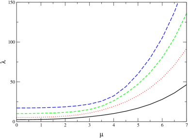
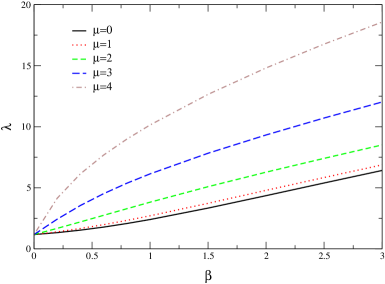
Figure 8: Left: Four smallest nonzero eigenvalues of the complex Fokker-Planck equation as a function of $\mu$ with $\beta=1$, $\kappa=1/2$. Right: Smallest nonzero eigenvalue as a function of $\beta$ for various values of $\mu$ at $\kappa=1/2$.

If the action and therefore the Langevin dynamics would be real, these results would be sufficient to explain the convergence of the observables towards the correct values as observed above, by employing Eq. (3.36) in the large $\theta$ limit. In the complex case we consider here, this is not immediately clear. Given the real Langevin equations,

$$\frac{\partial x}{\partial\theta}=K_{x}+\eta,\;\;\;\;\;\;\;\;\;\;\;\;\frac{\partial y}{\partial\theta}=K_{y},$$ (3.44)

one can also consider the real distribution $\rho(x,y,\theta)$, satisfying the Fokker-Planck equation

$$\frac{\partial}{\partial\theta}\rho(x,y,\theta)=L_{\rm FP}\rho(x,y,\theta),$$ (3.45)

with the real Fokker-Planck operator

$$L_{\rm FP}=\frac{\partial}{\partial x}\left(\frac{\partial}{\partial x}-K_{x}\right)-\frac{\partial}{\partial y}K_{y}.$$ (3.46)

After complexification, expectation values should then satisfy

$$\langle O(x+iy,\theta)\rangle_{\eta}=\int\frac{dxdy}{2\pi}\,\rho(x,y,\theta)O(x+iy).$$ (3.47)

In contrast to the complex distribution $P(x,\theta)$, the distribution $\rho(x,y,\theta)$ is real and has the interpretation as a probability distribution in the $x-y$ plane. The real and complex Fokker-Planck operators can be related, using

$$\frac{\partial}{\partial\theta}\langle O(x+iy,\theta)\rangle= \int\frac{dxdy}{2\pi}\,O(x+iy)L_{\rm FP}\rho(x,y,\theta)$$

$$= \int\frac{dxdy}{2\pi}\,O(x+iy)L_{\rm FP}^{c}\rho(x,y,\theta).$$ (3.48)

Here partial integration for finite $\theta$ is used as well as the analytic dependence of $O$ on $z=x+iy$. Eq. (3.48) suggests a relation between the spectrum of the complex and the real Fokker-Planck operator. However, we have not yet been able to show that a stationary solution of the real Fokker-Planck equation exists. We hope to come back to this issue in the future.

4 One link SU(3) model

4.1 Model

In this section we consider a one link model where the link $U$ is an element of SU(3). The partition function reads

$$Z=\int dU\,e^{-S_{B}}\det M,$$ (4.1)

with the bosonic part of the action

$$S_{B}=-\frac{\beta}{6}\left(\mbox{Tr}\,U+\mbox{Tr}\,U^{-1}\right).$$ (4.2)

For the fermion matrix we take

$$M=1+\kappa\left(e^{\mu}\sigma_{+}U+e^{-\mu}\sigma_{-}U^{-1}\right),$$ (4.3)

with $\sigma_{\pm}=\frac{1}{2}(1\!\!1\pm\sigma_{3})$. We use the Pauli matrix $\sigma_{3}$ rather than $\gamma$ matrices to avoid factors of 2. The determinant has the product form

$$\det M=\det\left(1+\kappa e^{\mu}U\right)\det\left(1+\kappa e^{-\mu}U^{-1}\right),$$ (4.4)

where the remaining determinants on the right-hand side are in colour space. In order to exponentiate the determinant, we use the identity, valid for $U\in$ SL($3,\mathbb{C}$),

$$\det\left(1+cU\right)=1+c\mbox{Tr}\,U+c^{2}\mbox{Tr}\,U^{-1}+c^{3}.$$ (4.5)

We find therefore that

$$\det M=e^{-S_{F}},\;\;\;\;\;\;\;\;S_{F}=-\ln{\cal M}^{(q)}-\ln{\cal M}^{(\bar{q})},$$ (4.6)

with the quark and anti-quark contributions

$${\cal M}^{(q)}= 1+3\kappa e^{\mu}P+3\kappa^{2}e^{2\mu}P^{-1}+\kappa^{3}e^{3\mu},$$ (4.7)

$${\cal M}^{(\bar{q})}= 1+3\kappa e^{-\mu}P^{-1}+3\kappa^{2}e^{-2\mu}P+\kappa^{3}e^{-3\mu}.$$ (4.8)

Here we introduced the Polyakov loop $P$ and its “conjugate” $P^{-1}$,

$$P=\frac{1}{3}\mbox{Tr}\,U,\;\;\;\;\;\;\;\;\;P^{-1}=\frac{1}{3}\mbox{Tr}\,U^{-1}.$$ (4.9)

Note that $PP^{-1}\neq 1$. At large $\mu$, the anti-quark contribution ${\cal M}^{(\bar{q})}\to 1$ and no longer contributes. However, the term is crucial to preserve the symmetry (2.6) and is in particular relevant at imaginary and small real $\mu$.

Observables are defined as

$$\langle O(U)\rangle=\frac{1}{Z}\int dU\,e^{-S_{B}(U)}\det M(U)\,O(U).$$ (4.10)

The observables we consider are the Polyakov loop $P$, the conjugate Polyakov loop $P^{-1}$ and the density $n$. The latter is determined by

$$\langle n\rangle=\frac{\partial\ln Z}{\partial\mu},$$ (4.11)

and reads

$$n= \frac{\partial\ln{\cal M}^{(q)}}{\partial\mu}+\frac{\partial\ln{\cal M}^{(\bar{q})}}{\partial\mu}$$

$$= 3\frac{\kappa e^{\mu}P+2\kappa^{2}e^{2\mu}P^{-1}+\kappa^{3}e^{3\mu}}{{\cal M}^{(q)}}-3\frac{\kappa e^{-\mu}P^{-1}+2\kappa^{2}e^{-2\mu}P+\kappa^{3}e^{-3\mu}}{{\cal M}^{(\bar{q})}}.\;\;\;\;$$ (4.12)

At zero chemical potential, the density vanishes while at large $\mu$ the density $n\to 3$, the maximal numbers of (spinless) quarks on the site.

In this model, expectation values can be obtained directly by numerical integration, allowing for a comparison with the results from stochastic quantization presented below. Since we only consider observables that depend on the conjugacy class of $U$, we only have to integrate over the conjugacy classes. These are parametrized by two angles $-\pi<\phi_{1},\phi_{2}\leq\pi$. The reduced Haar measure on the conjugacy classes $[U]$ reads

$$d[U]=\frac{1}{\cal N}\sin^{2}\left[\frac{1}{2}(\phi_{1}-\phi_{2})\right]\sin^{2}\left[\frac{1}{2}(\phi_{1}+2\phi_{2})\right]\sin^{2}\left[\frac{1}{2}(\phi_{2}+2\phi_{1})\right],$$ (4.13)

where ${\cal N}$ is a normalization constant. The matrix is parametrized as

$$U=\mbox{diag}\left(e^{i\phi_{1}},e^{i\phi_{2}},e^{-i(\phi_{1}+\phi_{2})}\right),$$ (4.14)

such that

$$S_{B}=-\frac{\beta}{3}\left[\cos(\phi_{1})+\cos(\phi_{2})+\cos(\phi_{1}+\phi_{2})\right],$$ (4.15)

and

$$P=\frac{1}{3}\left[e^{i\phi_{1}}+e^{i\phi_{2}}+e^{-i(\phi_{1}+\phi_{2})}\right],\;\;\;\;P^{-1}=\frac{1}{3}\left[e^{-i\phi_{1}}+e^{-i\phi_{2}}+e^{i(\phi_{1}+\phi_{2})}\right].$$ (4.16)

It is now straightforward to compute expectation values by numerical integration over $\phi_{1}$ and $\phi_{2}$.

4.2 Complex Langevin dynamics

In contrast to in the U(1) model, the Langevin dynamics is now defined in terms of matrix multiplication. We denote $U(\theta+\epsilon)=U^{\prime}$ and $U(\theta)=U$, where $\theta$ is again the Langevin time and consider the Langevin process,

$$U^{\prime}=R\,U,\;\;\;\;\;\;\;\;\;\;\;\;\;\;\;\;R=\exp\left[i\lambda_{a}\left(\epsilon K_{a}+\sqrt{\epsilon}\eta_{a}\right)\right].$$ (4.17)

Here $\lambda_{a}$ ($a=1,\ldots,8$) are the traceless, hermitian Gell-Mann matrices, normalized as $\mbox{Tr}\,\lambda_{a}\lambda_{b}=2\delta_{ab}$. The noise satisfies

$$\langle\eta_{a}\rangle=0,\;\;\;\;\;\;\;\;\;\langle\eta_{a}\eta_{b}\rangle=2\delta_{ab},$$ (4.18)

and the drift term reads

$$K_{a}=-D_{a}S_{\rm eff},\;\;\;\;\;\;\;\;\;\;\;\;S_{\rm eff}=S_{B}+S_{F}.$$ (4.19)

Differentiation is defined as

$$D_{a}f(U)=\frac{\partial}{\partial\alpha}f\left(e^{i\alpha\lambda_{a}}U\right)\Big{|}_{\alpha=0}.$$ (4.20)

In particular, $D_{a}U=i\lambda_{a}U$ and $D_{a}U^{-1}=-iU^{-1}\lambda_{a}$.

The explicit expressions for the drift terms are

$$K_{a}=K_{a}^{B}+K_{a}^{F},$$ (4.21)

with

$$K_{a}^{B}=-D_{a}S_{B}(U)= \frac{\beta}{2}\left(D_{a}P+D_{a}P^{-1}\right),$$ (4.22)

$$K_{a}^{F}=-D_{a}S_{F}(U)= 3\frac{\kappa e^{\mu}D_{a}P+\kappa^{2}e^{2\mu}D_{a}P^{-1}}{{\cal M}^{(q)}}+3\frac{\kappa e^{-\mu}D_{a}P^{-1}+\kappa^{2}e^{-2\mu}D_{a}P}{{\cal M}^{(\bar{q})}},$$

written in terms of

$$D_{a}P=\frac{i}{3}\mbox{Tr}\,\lambda_{a}U,\;\;\;\;\;\;\;\;\;\;\;\;D_{a}P^{-1}=-\frac{i}{3}\mbox{Tr}\,U^{-1}\lambda_{a}.$$ (4.24)

Let us first consider the case without chemical potential and take $U\in$ SU(3). Then it is easy to see that $K^{\dagger}_{a}=K_{a}$ and therefore $R^{\dagger}R=1\!\!1$. Moreover, since the Gell-man matrices are traceless, $\det R=1$. Therefore, if $U$ is an element of SU(3), it will remain in SU(3) during the Langevin process. The same results are found at finite imaginary chemical potential $\mu=i\mu_{I}$. At nonzero real $\mu$ on the other hand, we find that $R^{\dagger}R\neq 1\!\!1$, although $\det R=1$ still holds. Therefore $U$ will be an element of SL($3,\mathbb{C}$) during the Langevin evolution. If $U$ is parametrized as $U=\exp\left(i\lambda_{a}A_{a}/2\right)$, this implies that the gauge potentials $A_{a}$ are complex.

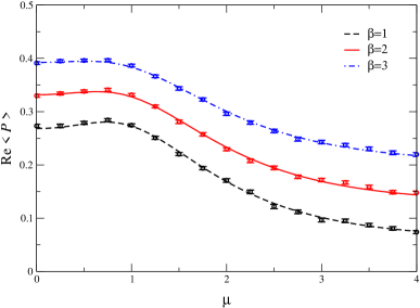
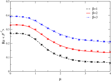
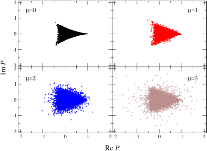
Figure 9: Real part of the Polyakov loop $\langle P\rangle$ (left) and the conjugate Polyakov loop $\langle P^{-1}\rangle$ (right) as a function of $\mu$ for three values of $\beta$ at fixed $\kappa=1/2$.

Figure 10: Scatter plot of the Polyakov loop for $\beta=1$, $\kappa=1/2$ and $\mu=0,1,2,3$.

We solved the Langevin process (4.17) numerically. The matrix $R$ is computed by exponentiating the complex traceless matrix $i\lambda_{a}\left(\epsilon K_{a}+\sqrt{\epsilon}\eta_{a}\right)$, employing Cardano’s method [37] for finding the eigenvalues. In Fig. 10 the real part of the Polyakov loop $\langle P\rangle$ and the conjugate Polyakov loop $\langle P^{-1}\rangle$ are shown as a function of $\mu$ for three values of $\beta$ at fixed $\kappa=1/2$. The lines are the ‘exact’ results obtained by numerically integrating over the angles $\phi_{1}$ and $\phi_{2}$, as discussed above. The symbols are obtained with complex Langevin dynamics, using the same Langevin stepsize and number of time steps as in the U(1) model ($\epsilon=5\times 10^{-5}$ and $5\times 10^{7}$ time steps). Errors are estimated with the jackknife procedure. Again, the imaginary part is zero analytically and consistent with zero within the error in the Langevin dynamics. Excellent agreement between the exact and the stochastic results can be seen.

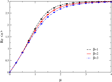
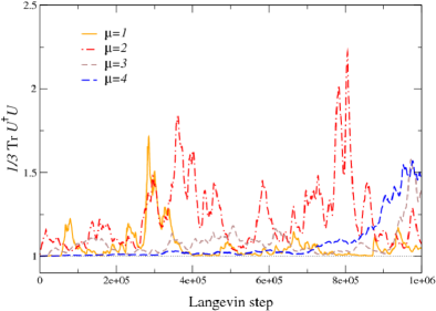
Figure 11: Left: Real part of the density $\langle n\rangle$. Right: Deviation from SU(3) during complex Langevin evolution: $\mbox{Tr}\,U^{\dagger}U/3$ as a function of Langevin step, for $\mu=1,2,3,4$ at $\beta=1,\kappa=1/2$.

Scatter plots of the Polyakov loop during the Langevin evolution are shown in Fig. 10 for four values of $\mu$ at $\beta=1$ and $\kappa=1/2$. Every point is separated from the previous one by 500 time steps. Note that the distribution is approximately symmetric under reflection $\mbox{Im\,}P\to-\mbox{Im\,}P$, ensuring that $\mbox{Im\,}\langle P\rangle=0$ within the error. We observe that the characteristic shape visible at $\mu=0$ becomes more and more fuzzy at larger $\mu$, but the average remains well defined for all values of $\mu$. The density is shown in Fig. 11 (left), with again good agreement between the exact and the stochastic results. We observe that saturation effects set in for smaller values of $\mu$ compared to the U(1) model, e.g. $n=n_{\rm max}/2=3/2$ already at $\mu\approx 1$.

During the complex Langevin evolution the matrix $U\in$ SL$(3,\mathbb{C})$. In order to quantify how much it deviates from SU(3), we may follow the evolution of

$$f(U)=\frac{1}{3}\mbox{Tr}\,U^{\dagger}U.$$ (4.25)

It is easy to show that $f(U)\geq 1$, with the equality in the case that $U\in$ SU(3). It provides therefore a good measure to quantify the deviation from SU(3). In Fig. 11 (right), we show this quantity during the Langevin evolution. We observe that the deviations from 1 are present but not too large. If $U$ is parametrized as $U=\exp\left(i\lambda_{a}A_{a}/2\right)$, this implies the imaginary parts of the gauge potentials $A_{a}$ do not become unbounded.

4.3 Phase of the determinant

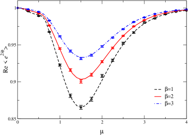
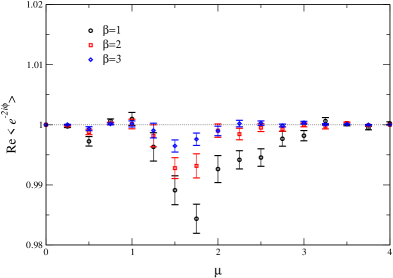
Figure 12: Left: Real part of $\langle e^{2i\phi}\rangle=\langle\det M(\mu)/\det M(-\mu)\rangle$. Right: Real part of $\langle\det M(-\mu)/\det M(\mu)\rangle$.

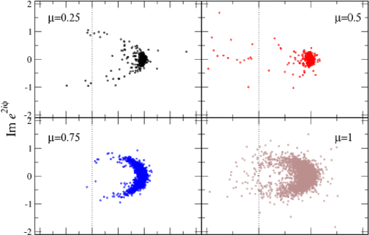
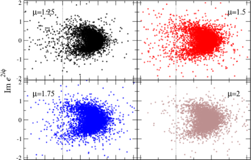
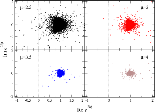
Figure 13: Scatter plot of $e^{2i\phi}=\det M(\mu)/\det M(-\mu)$ during the Langevin evolution, for $\beta=1$, $\kappa=1/2$ and $0.25\leq\mu\leq 4$.

As in the U(1) model, we study the phase of the determinant in the form

$$\langle e^{2i\phi}\rangle=\left\langle\frac{\det M(\mu)}{\det M(-\mu)}\right\rangle.$$ (4.26)

At zero chemical potential, the ratio is 1. Due to the SU(3) structure, however, the behaviour at large $\mu$ is qualitatively different. We find

$$\lim_{\mu\to\infty}\det M(\mu)= \kappa^{3}e^{3\mu}\left[1+3e^{-\mu}\left(\kappa+\kappa^{-1}\right)P^{-1}+{\cal O}(e^{-2\mu})\right],$$ (4.27)

$$\lim_{\mu\to\infty}\det M(-\mu)= \kappa^{3}e^{3\mu}\left[1+3e^{-\mu}\left(\kappa+\kappa^{-1}\right)P+{\cal O}(e^{-2\mu})\right],$$ (4.28)

such that

$$\lim_{\mu\to\infty}\frac{\det M(\mu)}{\det M(-\mu)}=1+3e^{-\mu}\left(\kappa+\kappa^{-1}\right)\left(P^{-1}-P\right)+{\cal O}(e^{-2\mu}).$$ (4.29)

As a result the average phase goes to 1 at large $\mu$ and not towards 0 as in the U(1) model. Therefore we expect the sign problem to become exponentially small in the saturation regime at large $\mu$.

We have computed the average phase factor and the results are shown in Fig. 12 (left). The lines are again the ‘exact’ results. As is clear from this plot, the sign problem is quite mild for all values of $\mu$, since the maximal deviation from 1 is less than 15%. In Fig. 12 (right) the ratio $\langle\det M(-\mu)/\det M(\mu)\rangle=Z(-\mu)/Z(\mu)$ is shown. Here we observe a small but systematic deviation from 1, more pronounced at smaller $\beta$ and intermediate $\mu$. However, we found that the deviation from 1 is reduced when continuing the Langevin evolution to larger and larger times. As in the U(1) model, this observable is the most sensitive and slowest converging quantity.

Scatter plots of the phase are presented in Fig. 13. At small chemical potential (top figure), there appears to be a similar structure as in the U(1) model, although not as pronounced. In the intermediate region (middle), the distribution is wider. At large $\mu$ (bottom), the distribution becomes narrow again, centered around $(1,0)$.

5 QCD at finite chemical potential

5.1 Hopping expansion

In this section we leave the one link models behind and consider QCD at chemical potential. The SU(3) gauge field contribution to the euclidean lattice action is

$$S_{B}[U]=-\beta\sum_{x}\mathop{\sum_{\mu,\nu}}_{\mu<\nu}\left(\frac{1}{6}\left[\mbox{Tr}\,U_{x,\mu\nu}+\mbox{Tr}\,U_{x,\mu\nu}^{-1}\right]-1\right),$$ (5.1)

with $\beta=6/g^{2}$. The plaquettes are defined as

$$U_{x,\mu\nu}=U_{x,\mu}U_{x+\hat{\mu},\nu}U^{-1}_{x+\hat{\nu},\mu}U^{-1}_{x,\nu},$$ (5.2)

and

$$U_{x,\mu\nu}^{-1}=U_{x,\nu\mu}.$$ (5.3)

The fermion matrix $M$ for Wilson fermions was already given in Eq. (2.7). The $\gamma$ matrices satisfy $\gamma_{\mu}^{\dagger}=\gamma_{\mu}$ and $\gamma_{\mu}^{2}=1\!\!1$. We use periodic boundary conditions in space and antiperiodic boundary conditions in the euclidean time direction; the temperature and the number of time slices $N_{\tau}$ are related as $T=1/N_{\tau}$ (the lattice spacing $a\equiv 1$). The fermion matrix obeys

$$M^{\dagger}(\mu)=\gamma_{5}M(-\mu)\gamma_{5},$$ (5.4)

such that the determinant obeys Eq. (2.6).

We consider the heavy quark limit, where all spatial hopping terms are ignored and only the temporal links in the fermion determinant are preserved. We write therefore

$$\det M\approx \det\left[1-\kappa\left(e^{\mu}\Gamma_{+4}U_{x,4}T_{4}+e^{-\mu}\Gamma_{-4}U_{x,4}^{-1}T_{-4}\right)\right]$$

$$= \det\left(1-2\kappa e^{\mu}U_{x,4}T_{4}\right)^{2}\det\left(1-2\kappa e^{-\mu}U_{x,4}^{-1}T_{-4}\right)^{2}$$

$$= \prod_{{\mathbf{x}}}\det\left(1+he^{\mu/T}{\cal P}_{{\mathbf{x}}}\right)^{2}\det\left(1+he^{-\mu/T}{\cal P}_{{\mathbf{x}}}^{-1}\right)^{2},$$ (5.5)

where we defined $h=(2\kappa)^{N_{\tau}}$ and the (conjugate) Polyakov loops are

$${\cal P}_{\mathbf{x}}=\prod_{\tau=0}^{N_{\tau}-1}U_{(\tau,{\mathbf{x}}),4},\;\;\;\;\;\;\;\;\;\;\;\;\;\;\;\;{\cal P}_{\mathbf{x}}^{-1}=\prod_{\tau=N_{\tau}-1}^{0}U_{(\tau,{\mathbf{x}}),4}^{-1}.$$ (5.6)

In the final line of Eq. (5.5) the determinant refers to colour space only. The $+$ sign appears because of the antiperiodic boundary conditions.

This approximation is motivated by the Heavy Dense Model considered e.g. in Refs. [30, 31, 32, 33, 34, 35, 36], in which the limit

$$\kappa\to 0,\;\;\;\;\;\;\;\;\mu\to\infty,\;\;\;\;\;\;\;\;\kappa e^{\mu}\;\;\mbox{fixed},$$ (5.7)

was taken. However, here also the backward propagating quark, with the inverse Polyakov loop, is kept in order to preserve the relation (2.6).

Using Eq. (4.5), the determinant can now be written as

$$\det M=e^{-S_{F}},\;\;\;\;\;\;\;\;\;\;\;\;S_{F}=-\sum_{\mathbf{x}}\left(2\ln{\cal M}^{(q)}_{\mathbf{x}}+2\ln{\cal M}^{(\bar{q})}_{\mathbf{x}}\right),$$ (5.8)

with the quark and anti-quark contributions

$${\cal M}^{(q)}_{\mathbf{x}}= 1+3he^{\mu/T}P_{{\mathbf{x}}}+3h^{2}e^{2\mu/T}P_{{\mathbf{x}}}^{-1}+h^{3}e^{3\mu/T},$$ (5.9)

$${\cal M}^{(\bar{q})}_{\mathbf{x}}= 1+3he^{-\mu/T}P_{{\mathbf{x}}}^{-1}+3h^{2}e^{-2\mu/T}P_{{\mathbf{x}}}+h^{3}e^{-3\mu/T},$$ (5.10)

where

$$P_{\mathbf{x}}=\frac{1}{3}\mbox{Tr}\,{\cal P}_{\mathbf{x}},\;\;\;\;\;\;\;\;\;\;\;\;P_{\mathbf{x}}^{-1}=\frac{1}{3}\mbox{Tr}\,{\cal P}_{\mathbf{x}}^{-1}.$$ (5.11)

The density is given by

$$\langle N\rangle=\sum_{\mathbf{x}}\langle n_{\mathbf{x}}\rangle=T\frac{\partial\ln Z}{\partial\mu},$$ (5.12)

and we find

$$n_{\mathbf{x}}= 2T\frac{\partial\ln{\cal M}^{(q)}_{\mathbf{x}}}{\partial\mu}+2T\frac{\partial\ln{\cal M}^{(\bar{q})}_{\mathbf{x}}}{\partial\mu}$$

$$= 6\frac{he^{\mu/T}P_{\mathbf{x}}+2h^{2}e^{2\mu/T}P^{-1}_{\mathbf{x}}+h^{3}e^{3\mu/T}}{{\cal M}^{(q)}_{\mathbf{x}}}$$ (5.13)

$$-6\frac{he^{-\mu/T}P^{-1}_{\mathbf{x}}+2h^{2}e^{-2\mu/T}P_{\mathbf{x}}+h^{3}e^{-3\mu/T}}{{\cal M}^{(\bar{q})}_{\mathbf{x}}}.$$

At zero chemical potential, the density vanishes while at large $\mu$ the density $n_{\mathbf{x}}\to 6$, the maximal numbers of quarks on a site.

5.2 Complex Langevin dynamics

The implementation of the Langevin dynamics follows closely the one discussed in the previous section on the SU(3) one link model. We denote $U_{x,\mu}(\theta+\epsilon)=U^{\prime}_{x,\mu}$ and $U_{x,\mu}(\theta)=U_{x,\mu}$, and consider the process

$$U^{\prime}_{x,\mu}=R_{x,\mu}\,U_{x,\mu},\;\;\;\;\;\;\;\;\;\;\;\;R_{x,\mu}=\exp\left[i\lambda_{a}\left(\epsilon K_{x\mu a}+\sqrt{\epsilon}\eta_{x\mu a}\right)\right],$$ (5.14)

with the noise satisfying

$$\langle\eta_{x\mu a}\rangle=0,\;\;\;\;\;\;\;\;\;\;\;\;\langle\eta_{x\mu a}\eta_{y\nu b}\rangle=2\delta_{\mu\nu}\delta_{ab}\delta_{xy}.$$ (5.15)

The drift term is

$$K_{x\mu a}=-D_{x\mu a}S[U].$$ (5.16)

Differentiation is defined as

$$D_{x\mu a}f(U)=\frac{\partial}{\partial\alpha}f\left(e^{i\alpha\lambda_{a}}U_{x,\mu}\right)\Big{|}_{\alpha=0}.$$ (5.17)

The drift term is written as

$$K_{x\mu a}=K_{x\mu a}^{B}+K_{x\mu a}^{F},$$ (5.18)

with the bosonic contribution

$$K_{x\mu a}^{B}= -D_{x\mu a}S_{B}[U]$$

$$= i\frac{\beta}{6}\sum_{\nu\neq\mu}\mbox{Tr}\,\!\left[\lambda_{a}U_{x\mu}C_{x,\mu\nu}-\overline{C}_{x,\mu\nu}U_{x\mu}^{-1}\lambda_{a}\right],$$ (5.19)

where

$$C_{x,\mu\nu}=U_{x+\hat{\mu},\nu}U^{-1}_{x+\hat{\nu},\mu}U^{-1}_{x,\nu}+U^{-1}_{x+\hat{\mu}-\hat{\nu},\nu}U^{-1}_{x-\hat{\nu},\mu}U_{x-\hat{\nu},\nu},$$ (5.20)

$$\overline{C}_{x,\mu\nu}=U_{x,\nu}U_{x+\hat{\nu},\mu}U^{-1}_{x+\hat{\mu},\nu}+U^{-1}_{x-\hat{\nu},\nu}U_{x-\hat{\nu},\mu}U_{x+\hat{\mu}-\hat{\nu},\nu}.$$ (5.21)

The fermionic contribution is

$$K_{x\mu a}^{F}=-D_{x\mu a}S_{F}[U]=\delta_{\mu 4}K^{F}_{xa},$$ (5.22)

with

$$K_{xa}^{F}=6\frac{he^{\mu/T}D_{xa}P_{{\mathbf{x}}}+h^{2}e^{2\mu/T}D_{xa}P_{{\mathbf{x}}}^{-1}}{{\cal M}^{(q)}_{{\mathbf{x}}}}+6\frac{he^{-\mu/T}D_{xa}P_{{\mathbf{x}}}^{-1}+h^{2}e^{-2\mu/T}D_{xa}P_{{\mathbf{x}}}}{{\cal M}^{(\bar{q})}_{{\mathbf{x}}}}.$$ (5.23)

The derivatives are

$$D_{xa}P_{{\mathbf{x}}}= D_{(\tau{\mathbf{x}})a}P_{{\mathbf{x}}}=\frac{i}{3}\mbox{Tr}\,\prod_{\tau^{\prime}=0}^{\tau-1}U_{(\tau^{\prime}{\mathbf{x}})4}\lambda_{a}\prod_{\tau^{\prime\prime}=\tau}^{N_{\tau}-1}U_{(\tau^{\prime\prime}{\mathbf{x}})4},$$ (5.24)

$$D_{xa}P_{{\mathbf{x}}}^{-1}= D_{(\tau{\mathbf{x}})a}P_{{\mathbf{x}}}^{-1}=-\frac{i}{3}\mbox{Tr}\,\prod_{\tau^{\prime}=N_{\tau}-1}^{\tau}U_{(\tau^{\prime}{\mathbf{x}})4}^{-1}\lambda_{a}\prod_{\tau^{\prime\prime}=\tau-1}^{0}U_{(\tau^{\prime\prime}{\mathbf{x}})4}^{-1}.$$ (5.25)

We have solved Eq. (5.14) numerically. A detailed analysis is postponed to a future publication; here we present some results for illustration purposes. We have used the temporal gauge, where only the last link differs from the identity,

$$U_{(N_{\tau}-1,{\mathbf{x}})4}=V_{{\mathbf{x}}},\;\;\;\;\;\;\;\;\;\;\;\;U_{(\tau,{\mathbf{x}})4}=1\!\!1\;\;\;\;(\tau\neq N_{\tau}-1).$$ (5.26)

To simplify the exponentiation we use the following updating factor in Eq. (5.14),

$${\tilde{R}}_{x,\mu}=\prod_{a={\rm Perm}(1,..,8)}e^{i\lambda_{a}\left(\epsilon K_{x\mu a}+\sqrt{\epsilon}\eta_{x\mu a}\right)},$$ (5.27)

with random ordering from sweep to sweep and where $K_{x\mu a}$ is complex. $R$ and ${\tilde{R}}$ only differ by terms of order $\epsilon^{2}$, which is the general systematic error of the Langevin algorithm. For the results shown here, we have employed Langevin stepsize $\epsilon=2\times 10^{-5}$ and 50000 iterations of 50 sweeps each, using ergodicity to calculate averages. Runaway trajectories have practically been eliminated by monitoring the drift and using adaptive step size. The lattice has size $4^{4}$, with $\beta=5.6$, $\kappa=0.12$. We have studied chemical potentials in the range $0.5\leq\mu\leq 0.9$, using $N_{f}=3$ fermion flavours.

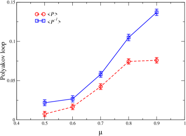
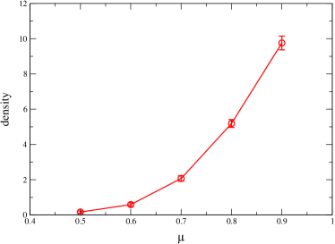
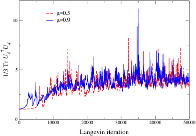
Figure 14: Real part of the Polyakov loop $\langle P\rangle$ and the conjugate Polyakov loop $\langle P^{-1}\rangle$ (left) and the density $\langle n\rangle$ (right) as a function of $\mu$ at $\beta=5.6$, $\kappa=0.12$ on a $4^{4}$ lattice, with $N_{f}=3$ flavours.

Figure 15: Deviation from SU(3): $\mbox{Tr}\,U_{4}^{\dagger}U_{4}/3$ during the Langevin evolution, for $\mu=0.5$ and $0.9$.

In Fig. 15 we present the real part of the Polyakov loop and the conjugate Polyakov loop (left) and the density (right). These results appear consistent with those obtained in Ref. [36] using reweighting techniques, although at this level of the study both statistics and thermalization are not yet optimal. Nevertheless we clearly see that at $\mu=0.5$ the system is in the low-density “confining” phase whereas for larger $\mu$ the density increases rapidly and both the direct and the conjugate Polyakov loops become nonzero, indicating “deconfinement”.

The deviation from SU(3) during the complex Langevin evolution is shown in Fig. 15, using $\mbox{Tr}\,U_{4}^{\dagger}U_{4}/3$ as the observable. After the initial thermalization stage, this quantity fluctuates around $3.5>1$. The fluctuations are similar for all values of the chemical potential we considered. Using spatial links $U_{i}$ rather than $U_{4}$ gives a similar result.

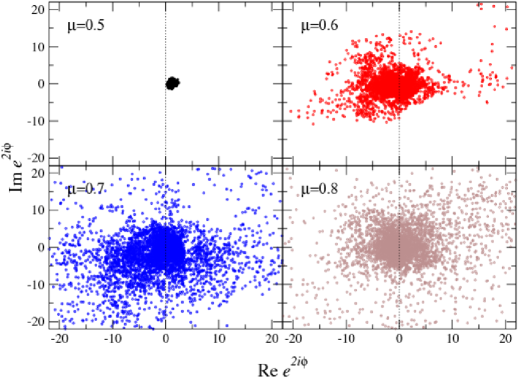
Figure 16: Scatter plot of $e^{2i\phi}=\det M(\mu)/\det M(-\mu)$ during the Langevin evolution for various values of $\mu$ at $\beta=5.6$, $\kappa=0.12$ on a $4^{4}$ lattice.

5.3 Phase of the determinant

We study the phase of the determinant as before. Scatter plots during the Langevin evolution are shown in Fig. 16, for $\mu=0.5,0.6,0.7$, and $0.8$. At the smallest value of $\mu$, the average phase factor is close to one; for the real part we find $0.91\pm 0.28$, while the imaginary part is consistent with zero ($0.009\pm 0.39$). At the larger values shown here, the distribution immediately becomes very wide and the average phase factor is consistent with zero (but with a large error). Note that the scale is very different compared to the one link model. Such an (apparently) abrupt change in the average phase factor when moving from a low-density to a high-density phase is somewhat reminiscent of what is found in random matrix studies, see e.g. Refs. [38, 39, 40].

At large chemical potential the average phase factor approaches 1 again. This follows from the behaviour of the determinant,

$$\lim_{\mu\to\infty}\det M(\mu)= \prod_{\mathbf{x}}h^{3}e^{3\mu/T}\left[1+3e^{-\mu/T}\left(h+h^{-1}\right)P_{\mathbf{x}}^{-1}+{\cal O}(e^{-2\mu/T})\right],\;\;\;\;$$ (5.28)

$$\lim_{\mu\to\infty}\det M(-\mu)= \prod_{\mathbf{x}}h^{3}e^{3\mu/T}\left[1+3e^{-\mu/T}\left(h+h^{-1}\right)P_{\mathbf{x}}+{\cal O}(e^{-2\mu/T})\right],\;\;\;\;$$ (5.29)

such that

$$\lim_{\mu\to\infty}\frac{\det M(\mu)}{\det M(-\mu)}=1+3e^{-\mu/T}\left(h+h^{-1}\right)\prod_{\mathbf{x}}\left(P_{\mathbf{x}}^{-1}-P_{\mathbf{x}}\right)+{\cal O}(e^{-2\mu/T}).$$ (5.30)

However, the values of the chemical potential we consider are not in that saturation region.

6 Summary and outlook

We have considered stochastic quantization for theories with a complex action due to finite chemical potential, and applied complex Langevin dynamics to U(1) and SU(3) one link models and QCD in the hopping expansion. In the latter, the full gauge dynamics is preserved but the fermion determinant is approximated. In all cases the complex determinant satisfies $\det M(\mu)=[\det M(-\mu)]^{*}$, as is the case in QCD. We studied the (conjugate) Polyakov loops, the density and the phase of the determinant. In the one link models excellent agreement between the numerical and exact results was obtained, for all values of $\mu$ ranging from zero to saturation.

In the one link models the phase of the determinant was studied in detail. Even when the phase factor varies significantly during the Langevin evolution, its distribution is well-defined and expectation values can be evaluated without problems. The sign problem does not appear to be an obstruction here. In QCD in the hopping expansion, first results indicate that the behaviour of the average phase factor changes abruptly when moving from the low-density to a high-density phase. Nevertheless, other observables (Polyakov loop, density) are still under control, even at larger chemical potential.

In the case of the U(1) model, we found strong hints why the sign problem does not appear to affect this method. We found that important features of classical flow and classical fixed points are largely independent of the chemical potential. The presence of $\mu$ changes the complex Langevin dynamics only quantitatively but not qualitatively, even when the average phase factor of the determinant becomes very small. Moreover, a study of the complex Fokker-Planck equation shows that all nonzero eigenvalues are real and positive, also in the presence of a nonzero chemical potential. An open question concerns the relationship between the stationary solution of the complex Fokker-Planck operator and its real counterpart. The structure in the U(1) model responsible for these results is related to symmetry properties of the action and the determinant. Therefore, it may be envisaged that they carry over to the more complicated cases.

There are many directions into which this work can be extended. In the U(1) model, considerable insight could be obtained (semi-)analytically. It will be interesting to extend this analysis to more complicated theories. It will also be useful to perform further tests of the method in other simple models sharing relevant features with QCD at finite $\mu$. Concerning QCD in the hopping expansion, for which we presented first results here, a more systematic study stays ahead. One way to test the approach is to also perform (real) Langevin dynamics at imaginary chemical potential, which goes smoothly and without runaway and convergence problems, and perform an analytical continuation. Finally, it will be interesting to apply this method to QCD both at large density as well as in the region of small chemical potential around the crossover temperature. Here it may shed light on the (non)existence of the critical point, in a setup which is manifestly independent from the other approaches available in this region. It should be noted that the Langevin method only requires the derivative of the determinant, and not the determinant itself.

Acknowledgments. We are indebted to Erhard Seiler who collaborated during part of this work and contributed many important insights. G.A. thanks Simon Hands, Biagio Lucini and Asad Naqvi for discussion. This work was initiated while both authors were participating in the programme on Nonequilibrium Dynamics in Particle Physics and Cosmology at the Kavli Institute for Theoretical Physics in Santa Barbara and supported in part by the National Science Foundation under Grant No. PHY05-51164. We thank the organizers for this opportunity. G.A. wants to thank the organizers of the programme on New Frontiers in QCD 2008: Fundamental Problems in Hot and/or Dense Matter at the Yukawa Institute for Theoretical Physics in Kyoto where part of this work was carried out. I.-O. S. thanks the Max-Plank-Institute (Werner Heisenberg Institute) Munich for repeated hospitality during which work for this study was carried out. G.A. is supported by an STFC Advanced Fellowship.

Appendix A Fokker-Planck equation in Minkowski time

In Refs. [26, 27, 28] stochastic quantization was applied to nonequilibrium quantum dynamics in real time. For completeness, we give here the analysis of the corresponding complex Fokker-Planck equation for the one link U(1) model.

Consider the following partition function in Minkowski time,

$$Z_{p}=\int_{-\pi}^{\pi}\frac{dx}{2\pi}\,e^{iS_{p}},\;\;\;\;\;\;\;\;\;\;\;\;\;\;\;\;S_{p}=\beta\cos x+px.$$ (A.1)

The term $px$, with $p$ integer, is a reweighting term, used to stabilize the Langevin dynamics (see also Ref. [28]). The Fokker-Planck equation for the (complex) distribution $P_{p}$ reads

$$\frac{\partial}{\partial\theta}P_{p}(x,\theta)= \frac{\partial}{\partial x}\left(\nu\frac{\partial}{\partial x}-i\frac{\partial S_{p}}{\partial x}\right)P_{p}(x,\theta)$$

$$= \nu P_{p}^{\prime\prime}(x,\theta)+i\left[\beta\sin(x)-p\right]P_{p}^{\prime}(x,\theta)+i\beta\cos(x)P_{p}(x,\theta).$$ (A.2)

Here $\nu$ is essentially the normalization of the noise: for $\nu=1$ we have the full quantum case, for $\nu=0$ we obtain the classical evolution (which is equivalent to taking $\beta$ and $p$ to $\infty$).

To continue we discretize $x$ as $x_{l}=2\pi l/N$, with $-(N-1)/2\leq l\leq N/2$, and define the modes as

$${\tilde{P}}_{p}(n,\theta)= \frac{1}{N}\sum_{l=-(N-1)/2}^{N/2}e^{inx_{l}}P_{p}(x_{l},\theta),$$ (A.3)

$$P_{p}(x_{l},\theta)= \sum_{n=-(N-1)/2}^{N/2}e^{-inx_{l}}{\tilde{P}}_{p}(n,\theta).$$ (A.4)

The Fokker-Planck equation for the modes $\tilde{P}_{p}(n,\theta)$ then reads

$$\frac{\partial}{\partial\theta}{\tilde{P}}_{p}(n,\theta)= -\left[\nu\frac{N^{2}}{\pi^{2}}\sin^{2}(k_{n}/2)+p\frac{N}{2\pi}\sin(k_{n})\right]{\tilde{P}}_{p}(n,\theta)$$ (A.5)

$$+i\frac{\beta}{2}\frac{N}{2\pi}\left[\sin(k_{n+1}){\tilde{P}}_{p}(n+1,\theta)-\sin(k_{n-1}){\tilde{P}}_{p}(n-1,\theta)\right]$$

$$-i\frac{\beta}{2}\left[{\tilde{P}}_{p}(n+1,\theta)-{\tilde{P}}_{p}(n-1,\theta)\right],$$

where $k_{n}=2\pi n/N$. For small $n/N$ this reduces to

$$\frac{\partial}{\partial\theta}{\tilde{P}}_{p}(n,\theta)=-(\nu n^{2}+pn){\tilde{P}}_{p}(n,\theta)+\frac{n}{2}i\beta\left[{\tilde{P}}_{p}(n+1,\theta)-{\tilde{P}}_{p}(n-1,\theta)\right],$$ (A.6)

which can be obtained directly from the continuum Fokker-Planck equation before discretizing $x$. Extension to general (complex) $\beta=\beta_{R}+i\beta_{I}$ and $p=p_{R}+ip_{I}$ is straightforward. In the following no explicit $\nu$ means $\nu=1$.

From averages with the distribution $P$ we obtain

$$\langle e^{iqx}\rangle_{p}= \frac{\int_{-\pi}^{\pi}dx\,e^{iqx}P_{p}(x,\theta)}{\int_{-\pi}^{\pi}dx\,P_{p}(x,\theta)}=\frac{{\tilde{P}}_{p}(q,\theta)}{{\tilde{P}}_{p}(0,\theta)},$$ (A.7)

$$\langle e^{iqx}\rangle_{0}= \frac{\int_{-\pi}^{\pi}dx\,e^{iqx}P_{0}(x,\theta)}{\int_{-\pi}^{\pi}dx\,P_{0}(x,\theta)}=\frac{\int_{-\pi}^{\pi}dx\,e^{i(q-p)x}P_{p}(x,\theta)}{\int_{-\pi}^{\pi}dx\,e^{-ipx}P_{p}(x,\theta)}=\frac{{\tilde{P}}_{p}(q-p,\theta)}{{\tilde{P}}_{p}(-p,\theta)}.$$ (A.8)

Notice that $p$ and $q$ (both integers) are interchangeable. This implies that simulations can be performed at $p=0$, while Eqs. (A.7) – (A.8) can be used to obtain $P_{p}$ for any $p$.

Similar to the procedure of Sec. 3.4, we have solved the complex Fokker-Planck equation numerically for the modes $\tilde{P}_{p}(n,\theta)$. In contrast to the finite $\mu$ case, these modes are now complex in general. For example, for even (odd) $p$ even (odd) modes are real and odd (even) modes are imaginary, in agreement with the symmetries of the action. We further find that for $p>0$ the solution for positive modes converges correctly, but negative modes diverge, and vice versa. The numerical solution for $p=0$ converges quickly to the values determined by $e^{iS_{0}}$, when $0\leq\beta\lesssim 2.3$. In Fig. 17 (left) we show the Langevin time dependence of some modes when $\beta=1$, $p=0$. Using the asymptotic values for the modes and Eqs. (A.7) – (A.8), we can reconstruct $P_{p}(x)$, which agrees nicely with $e^{iS_{p}(x)}$. The Langevin simulation itself also yields good results for the expectation values when $p\neq 0$ or at $p=0$, provided reweighting from $p\neq 0$ is used. For a more thorough discussion of the conditions for convergence of the Langevin simulation, see Ref. [28].

Again further insight can be obtained from the eigenvalues, determined by the eigenvalue equation

$$n(n+p)\tilde{P}_{p}(n)+\frac{n}{2}i\beta\left[\tilde{P}_{p}(n+1)-\tilde{P}_{p}(n-1)\right]=\lambda\tilde{P}_{p}(n).$$ (A.9)

If $\lambda\neq 0$, $P_{p}(0)$ vanishes and the sequences for $n>0$ and $n<0$ split again in two. Positive and negative $n$ are related by changing the sign of $p$. In Fig. 17 we show the smallest nonzero eigenvalue for the positive $n$ sequence for five values of $p$. In contrast to the finite $\mu$ case, we find that eigenvalues may be negative, depending on the value of $p$ and $\beta$, indicating the possibility of problems with convergence and stability. This corroborates the above observations.

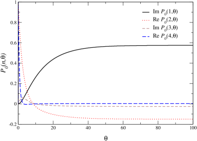
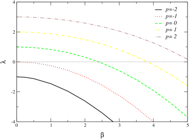
Figure 17: Complex Fokker-Planck equation for Minkowski dynamics. Left: Langevin time dependence of the modes $\tilde{P}_{0}(n,\theta)$ for various values of $n$, with $\beta=1$, $p=0$. Right: Smallest nonzero eigenvalue of the complex Fokker-Planck equation as a function of $\beta$ for various values of the reweighting parameter $p$.

Finally, one may also study the real Fokker-Planck equation to obtain the true probability distribution $\rho_{p}(x,y,\theta)$ and its modes. For an analytic function $O(z)$ we have

$$\int\frac{dxdy}{2\pi}\,\rho_{p}(x,y,\theta)O(x+iy)=\int\frac{dx}{2\pi}\,P_{p}(x,\theta)O(x),$$ (A.10)

hence, in particular,

$$\int\frac{dxdy}{2\pi}\,\rho_{p}(x,y,\theta)e^{inx-ny}=\int dy\,e^{-ny}{\tilde{\rho}}_{p}(n,y,\theta)=\int\frac{dx}{2\pi}\,P_{p}(x,\theta)e^{inx}={\tilde{P}}_{p}(n,\theta).$$ (A.11)

The expectation values with $\rho_{p}$ should represent the averages over the Langevin process itself. Even when the latter converge to the correct values, the real Fokker-Planck equation does not show good behaviour, however. We thus have the situation that we find agreement between the complex Fokker-Planck equation (with the corresponding complex distribution $P$) and the actual Langevin process, while the true probability distribution $\rho_{p}$, which formally mediates between the former two, appears more difficult to control.

References

- [1] Z. Fodor and S. D. Katz, Phys. Lett. B 534 (2002) 87 [hep-lat/0104001].
- [2] Z. Fodor and S. D. Katz, JHEP 0203 (2002) 014 [hep-lat/0106002].
- [3] Z. Fodor, S. D. Katz and K. K. Szabo, Phys. Lett. B 568 (2003) 73 [hep-lat/0208078].
- [4] Z. Fodor and S. D. Katz, JHEP 0404 (2004) 050 [hep-lat/0402006].
- [5] C. R. Allton et al., Phys. Rev. D 66 (2002) 074507 [hep-lat/0204010].
- [6] C. R. Allton, S. Ejiri, S. J. Hands, O. Kaczmarek, F. Karsch, E. Laermann and C. Schmidt, Phys. Rev. D 68 (2003) 014507 [hep-lat/0305007].
- [7] C. R. Allton et al., Phys. Rev. D 71 (2005) 054508 [hep-lat/0501030].
- [8] R. V. Gavai and S. Gupta, Phys. Rev. D 68 (2003) 034506 [hep-lat/0303013].
- [9] P. de Forcrand and O. Philipsen, Nucl. Phys. B 642 (2002) 290 [hep-lat/0205016].
- [10] P. de Forcrand and O. Philipsen, Nucl. Phys. B 673 (2003) 170 [hep-lat/0307020].
- [11] P. de Forcrand and O. Philipsen, JHEP 0701 (2007) 077 [hep-lat/0607017].
- [12] M. D’Elia and M. P. Lombardo, Phys. Rev. D 67 (2003) 014505 [hep-lat/0209146].
- [13] S. Kratochvila and P. de Forcrand, PoS LAT2005 (2006) 167 [hep-lat/0509143].
- [14] S. Ejiri, arXiv:0804.3227 [hep-lat].
- [15] Z. Fodor, S. D. Katz and C. Schmidt, JHEP 0703 (2007) 121 [hep-lat/0701022].
- [16] G. Parisi and Y. s. Wu, Sci. Sin. 24 (1981) 483.
- [17] For a review, see P. H. Damgaard and H. Huffel, Phys. Rept. 152 (1987) 227.
- [18] G. Parisi, Phys. Lett. B 131 (1983) 393.
- [19] J. R. Klauder and W. P. Petersen, SIAM J. Numer. Anal. 22 (1985) 1153.
- [20] J. R. Klauder and W. P. Petersen, J. Stat. Phys. 39 (1985) 53.
- [21] H. Gausterer and J. R. Klauder, Phys. Rev. D 33 (1986) 3678.
- [22] F. Karsch and H. W. Wyld, Phys. Rev. Lett. 55 (1985) 2242.
- [23] E. M. Ilgenfritz, Phys. Lett. B 181 (1986) 327.
- [24] N. Bilic, H. Gausterer and S. Sanielevici, Phys. Rev. D 37 (1988) 3684.
- [25] J. Ambjorn, M. Flensburg and C. Peterson, Nucl. Phys. B 275 (1986) 375.
- [26] J. Berges and I. O. Stamatescu, Phys. Rev. Lett. 95 (2005) 202003 [hep-lat/0508030].
- [27] J. Berges, S. Borsanyi, D. Sexty and I. O. Stamatescu, Phys. Rev. D 75 (2007) 045007 [hep-lat/0609058].
- [28] J. Berges and D. Sexty, Nucl. Phys. B 799 (2008) 306 [0708.0779 [hep-lat]].
- [29] P. Hasenfratz and F. Karsch, Phys. Lett. B 125 (1983) 308.
- [30] I. Bender et al., Nucl. Phys. Proc. Suppl. 26 (1992) 323.
- [31] J. Engels, O. Kaczmarek, F. Karsch and E. Laermann, Nucl. Phys. B 558 (1999) 307 [hep-lat/9903030].
- [32] T. C. Blum, J. E. Hetrick and D. Toussaint, Phys. Rev. Lett. 76 (1996) 1019 [hep-lat/9509002].
- [33] G. Aarts, O. Kaczmarek, F. Karsch and I. O. Stamatescu, Nucl. Phys. Proc. Suppl. 106 (2002) 456 [hep-lat/0110145].
- [34] R. Hofmann and I. O. Stamatescu, Nucl. Phys. Proc. Suppl. 129 (2004) 623 [hep-lat/0309179].
- [35] K. Fukushima and Y. Hidaka, Phys. Rev. D 75 (2007) 036002 [hep-ph/0610323].
- [36] R. De Pietri, A. Feo, E. Seiler and I. O. Stamatescu, Phys. Rev. D 76 (2007) 114501 [0705.3420 [hep-lat]].
- [37] Abramowitz, M. and Stegun, I. A. (Eds.), Handbook of Mathematical Functions, New York: Dover, p. 17, 1972.
- [38] K. Splittorff and J. J. M. Verbaarschot, Phys. Rev. Lett. 98 (2007) 031601 [hep-lat/0609076].
- [39] J. Han and M. A. Stephanov, arXiv:0805.1939 [hep-lat].
- [40] K. Splittorff, arXiv:hep-lat/0505001.
- [41] E. Seiler and I.-O. Stamatescu, unpublished (2007).