Deep inelastic scattering and prompt photon production within the framework of quark Reggeization hypothesis

Abstract

We study $ep$ deep inelastic scattering and the inclusive production of prompt photon within the framework of the quasi-multi-Regge-kinematic approach, applying the quark Reggeization hypothesis. We describe structure functions $F_{2}$ and $F_{L}$ supposing that a virtual photon scatters on a Reggeized quark from a proton, via the effective gamma-Reggeon-quark vertex. It is shown that the main mechanism of the inclusive prompt photon production in $p\bar{p}$ collisions is the fusion of a Reggeized quark and a Reggeized antiquark into a photon, via the effective Regeon-Reggeon-gamma vertex. We describe the inclusive photon transverse momentum spectra measured by the CDF and D0 Collaborations within errors and without free parameters, using the Kimber-Martin-Ryskin unintegrated quark and gluon distribution functions in a proton.

I Introduction

It is well known, that studies of lepton deep inelastic scattering (DIS) and production of photons with large transverse momenta producing in the hard interaction between two partons in hadron collisions, so called prompt photon production, provide precision tests of perturbative quantum chromodynamics (QCD) as well as information on the parton densities within protons.

Also these studies are our potential for the observation of a new dynamical regime, namely the high-energy Regge limit, which is characterized by the following condition $\sqrt{S}>>\mu>>\Lambda_{QCD}$, where $\sqrt{S}$ is the total collision energy in the center of mass reference frame, $\Lambda_{QCD}$ is the asymptotic scale parameter of QCD, $\mu$ is the typical energy scale of the hard interaction. At this high energy limit, the contribution from the partonic subprocesses involving $t-$channel parton (quark or gluon) exchanges to the production cross section can become dominant. In the region under consideration, the transverse momenta of the incoming partons and their off-shell properties can no longer be neglected, and we deal with ”Reggeized” $t-$channel partons.

The theoretical frameworks for this kind of high-energy phenomenology are the $k_{T}-$factorization approach GribovLevinRyskin ; CollinsEllis ; CataniCH and the quasi-multi-Regge kinematics (QMRK) approach FadinLipatov96 . Our previous analysis of charmonium and bottomonium production at the Fermilab Tevatron and DESY HERA Colliders using the high-energy factorization scheme KniehlSaleevVasin has shown the appreciation of the method even at the leading order (LO) in the strong-coupling constant $\alpha_{s}$ in comparison with the experimental data. We have found that essential features produced by the high-energy factorization scheme at LO are being at next-to-leading (NLO) in the conventional collinear parton model.

On the contrary the $k_{T}-$factorization scheme, based on the well known prescription for off-shell $t-$channel gluons CollinsEllis , the QMRK approach seems to be more proper theoretically Lipatov95 . In this approach we work with gauge invariant amplitudes and use the factorization hypothesis, which is proved in the leading-logarithmic-approximation (LLA). Recently it was shown, that the calculation at the NLO in the strong coupling constant within the framework of the QMRK approach can be done NLO .

In this paper we study the $ep$ DIS and the inclusive production of prompt photon within the framework of the QMRK approach, applying the quark Reggeization hypothesis FadinSherman . We describe DIS structure functions $F_{2}$ and $F_{L}$ suggesting that a virtual photon scatters on a Reggeized quarks from a proton, via the effective gamma-Reggeon-quark vertices. It is shown that the main mechanism of the inclusive prompt photon production in $p\bar{p}$ collisions is the fusion of a Reggeized quark and a Reggeized antiquark into a photon, via the effective Reggeon-Reggeon-gamma vertices. We describe the inclusive photon transverse momentum and pseudorapidity spectra measured by the D0D018 ; D0196 , and CDFCDF18 Collaborations within errors and without free parameters, using Kimber-Martin-Ryskin unintegrated KMR quark and gluon distribution functions in a proton. In case of prompt photon production we compare our results with another ones obtained recently in the $k_{T}-$factorization approach KMRgamma ; ZotovLipatovGamma ; SzczurekGamma , in detail.

This paper is organized as follows. In Sec. II, the relevant Reggeon-Reggeon-Particle (RRP) and Particle-Reggeon-Particle (PRP) effective vertices are written and discussed. In Sec. III, we consider $ep$ DIS in the QMRK approach, applying the quark Reggeization hypothesis. In Sec. IV, we describe in the high-energy factorization scheme the inclusive photon production at the Tevatron Collider both directly via the effective Reggeon-Reggeon-gamma vertices, and in the quark fragmentation into a photon via the Reggeon-Reggeon-Particle vertex. In Sec. V, we discuss and compare the relevant approaches used in the another studies within the $k_{T}-$factorization approach. In Sec. VI, we summarize our conclusions.

II Basic Formalism

In the phenomenology of strong interactions at high energies, it is necessary to describe the QCD evolution of the parton distribution functions of colliding particles starting with some scale $\mu_{0}$, which controls a non-perturbative regime, to the typical scale $\mu$ of the hard-scattering processes, which is typically of the order of the transverse mass $M_{T}=\sqrt{M^{2}+|{\bf p}_{T}|^{2}}$ of the produced particle with mass $M$ and transverse momentum ${\bf p}_{T}$. In the region of very high energies, in so-called Regge limit, the typical ratio $x=\mu/\sqrt{S}$ becomes very small, $x\ll 1$. That leads to large logarithmic contributions of the type $[\alpha_{s}\ln(1/x)]^{n}$ in the resummation procedure, which is described by the BFKL evolution equation BFKL for an unintegrated gluon (quark) distribution function $\Phi_{g,q}(x,|{\bf q}_{T}|^{2},\mu^{2})$. Correspondingly, in the QMRK approach FadinLipatov96 the initial-state $t$-channel gluons and quarks are considered as Reggeons, or Reggeized gluons $(R)$ and Reggeized quarks $(Q)$. They are off-mass shell and carry finite transverse two-momenta ${\bf q}_{T}$ with respect to the hadron beam from which they stem.

Recently, in the Ref. KTAntonov , the Feynman rules for the effective theory based on the non-abelian gauge-invariant action Lipatov95 were derived for the induced and some important effective vertices. However, these rules include processes with Reggeized gluons in the initial state only. In case of $t$-channel quark exchange processes such rules are unknown today and it is necessary to construct effective vertices with the Reggeized quarks, using QMRK approach prescriptions, every time from the begining. Of course, a certain set of Reggeon-Reggeon-Particle effective vertices are known, for example for the transitions $RR\to g$ LipatovFadin89 and $Q\bar{Q}\to g$ FadinSherman .

Roughly speaking, the Reggeization of amplitudes is a trick, which gives an opportunity to take into account efficiently large radiative corrections to the processes under Regge limit condition beyond the collinear approximation. The particle Reggeization is known in high energy quantum electrodynamics (QED) for electrons only GellMann and for gluons and quarks in QCD BFKL ; FadinSherman .

Contrary to the usual QCD vertices such as, for example, quark-quark-gluon vertex for which we can draw a definite set of Feynman diagrams with perfectly defined rules for the calculation of their contributions, we have no similar rules for the Reggeized quark vertices. These vertices are extracted from the comparison of radiative corrections to the scattering amplitudes with their Reggeized forms FadinFiore . Details of a reduction procedure from the initial set of diagrams with the on-shell collinear quarks or gluons to one effective Reggeon-Reggeon-Particle (or Particle-Reggeon-Particle) vertex can be found, for example, in the following papers FadinFiore ; LipatovFadin89 . We will use this method for the gamma-Reggeon-quark $(\gamma^{\star}Q\to q)$ vertex, which will be used in our calculations below.

Thus, the effective Reggeon-Reggeon-gluon (or Reggeon-Reggeon-photon) vertex $C_{\bar{Q}Q}^{g(\gamma)}(q_{1},q_{2})$ can be extracted from any amplitude of the $g(\gamma)$ production in the QMRK approach. In the simple case, they can be extracted from the amplitude $A_{\bar{q}q}^{g(g)g}$, which describes gluon (photon) production in the process:

$$q(p_{1})+\bar{q}(p_{2})\to g(p_{1}^{\prime})+g(k)+g(p_{2}^{\prime}).$$ (1)

At the high energy limit this process is described by a set of ladder type Feynman quark-exchange diagrams, which are presented in the Fig. 1. For the external gluon we use physical polarizations with different gauge fixing conditions for gluons moving along $p_{1}$ and $p_{2}$ , thus if the gluon momentum $p_{1}^{\prime}$ has a large component along $p_{1}$, its polarization vector $e(p_{1}^{\prime})$ satisfies equations $e(p_{1}^{\prime})p_{1}^{\prime}=e(p_{1}^{\prime})p_{2}=0$. The Reggeized form of the amplitude is expressed as follows:

$$A_{\bar{q}q}^{g(g)g}=2s\Gamma_{\bar{q}g}^{\bar{Q}}\frac{1}{t_{1}}C_{\bar{Q}Q}^{g}\frac{1}{t_{2}}\Gamma_{qg}^{Q},$$ (2)

where $t_{1}=(p_{1}-p_{1}^{\prime})^{2}$, $t_{2}=(p_{2}-p_{2}^{\prime})^{2}$, $s=2(p_{1}p_{2})$, $\Gamma_{\bar{q}g}^{\bar{Q}}$ and $\Gamma_{qg}^{Q}$ are the LO Particle-Particle-Reggeon vertices, see Ref. FadinFiore . The effective vertex $C_{\bar{Q}Q}^{g}(q_{1},q_{2})$, which describes the production of a single gluon with the momentum $k(g)=q_{1}(Q)+q_{2}(\bar{Q})$ in the Reggeized quark and Reggeized antiquark annihilation was obtained in Ref. FadinSherman ; FadinBogdan and it can be presented, omitting the color and Lorentz indices in the left side, as follows:

$$C_{\bar{Q}Q}^{g}(q_{1},q_{2})=D_{a}^{\mu}(q_{1},q_{2})=-g_{s}T^{a}\left(\gamma^{\mu}-\frac{2P_{1}^{\mu}}{x_{2}S}\hat{q_{2}}-\frac{2P_{2}^{\mu}}{x_{1}S}\hat{q_{1}}\right),$$ (3)

where $P_{1,2}$ are colliding hadron momenta, $P_{(1,2)}=E_{(1,2)}(1,\vec{0},\pm 1)$ and $S=2(P_{1}P_{2})=4E_{1}E_{2}$. The Reggeized quark momenta are $q_{1}=x_{1}P_{1}+q_{1T}$, $q_{2}=x_{2}P_{2}+q_{2T}$, and $q_{(1,2)T}=(0,\vec{q}_{(1,2)T},0)$. It is obviously that this vertex satisfies the gauge invariant condition $D_{a}^{\mu}(q_{1},q_{2})k_{\mu}=0$.

The same as for the gluon production, the effective vertex for the photon production can be written in the form:

$$C_{\bar{Q}Q}^{\gamma}(q_{1},q_{2})=F^{\mu}(q_{1},q_{2})=-ee_{q}\left(\gamma^{\mu}-\frac{2P_{1}^{\mu}}{x_{2}S}\hat{q_{2}}-\frac{2P_{2}^{\mu}}{x_{1}S}\hat{q_{1}}\right),$$ (4)

where $e=\sqrt{4\pi\alpha}$ is the electromagnetic coupling constant, $e_{q}$ is the quark electric charge.

The effective vertex $C_{RR}^{g}(q_{1},q_{2})$, which describes the production of a single gluon in the collision of two Reggeized gluons has the following form LipatovFadin89 :

$$C_{RR}^{g}(q_{1},q_{2})=W_{abc}^{\mu}(q_{1},q_{2})=-g_{s}f_{abc}\left((q_{2}-q_{1})^{\mu}+2P_{1}^{\mu}(x_{1}+\frac{q_{1}^{2}}{x_{2}S})-2P_{2}^{\mu}(x_{2}+\frac{q_{2}^{2}}{x_{1}S})\right).$$ (5)

The effective vertex, which describes the production of a quark with the momentum $k=q_{1}(\gamma^{\star})+q_{2}(Q)$ in a virtual photon collision with a Reggeized quark can be extracted from the amplitude, which is described by the two diagrams presented in Fig. 2, and it is written as follows

$$C_{\gamma Q}^{q}(q_{1},q_{2})=G^{\mu}(q_{1},q_{2})=-ee_{q}\left(\frac{q_{1}^{2}}{q_{1}^{2}+q_{2}^{2}}\gamma^{\mu}-\frac{2k^{\mu}}{q_{1}^{2}+q_{2}^{2}}\hat{q_{2}}+\frac{2q_{2}^{2}x_{2}P_{2}^{\mu}}{(q_{1}^{2}+q_{2}^{2})^{2}}\hat{q_{2}}\right),$$ (6)

where $q_{2}=x_{2}P_{2}+q_{2T}$ is the Reggeized quark four-momentum and the gauge invariance condition is given by $G^{\mu}(q_{1},q_{2})q_{1\mu}=0.$

The effective Reggeon-Reggeon-Particle vertex, which describes the production of a quark with the momentum $k(q)=q_{1}(Q)+q_{2}(R)$ in the Reggeized quark and Reggeized gluon collision can be presented as follows

$$C_{RQ}^{q}(q_{1},q_{2})=V(q_{1},q_{2})=-g_{s}T^{a}\hat{\varepsilon}_{T}(q_{2}),$$ (7)

where $\hat{\varepsilon}_{T}(q_{2})=\gamma_{\mu}\varepsilon^{\mu}(q_{2})$ and $\varepsilon^{\mu}(q_{2})=\displaystyle{\frac{q_{2T}^{\mu}}{|\vec{q}_{2T}|}}$. Let us note, that contrary to the definition used in the Ref. FadinBogdan in the relevant cases, we don’t include quark spinors in the our formulas for the effective vertices (3)-(7).

III Deep inelastic scattering and quark Reggeization

In this part we consider electron (positron) DIS on a proton at high energy in the framework of the quark Reggeization hypothesis. At first, to write down the conventional kinematic DIS formulas we define relevant four-momenta: $P_{e}$ is the electron initial four-momentum, $P_{N}$ is the proton four-momentum, $q_{1}$ is the virtual photon four-momentum, $q_{2}$ is the Reggeized quark four-momentum. The invariant variables are defined as follows:

$$S_{eN}=2(P_{e}P_{N}),\quad y=\displaystyle{\frac{(q_{1}P_{N})}{(P_{e}P_{N})}},\quad x_{B}=\frac{Q^{2}}{2(q_{1}P_{N})},\quad Q^{2}=-q_{1}^{2}.$$ (8)

As usual, we write the differential cross section as a convolution of the lepton tensor $L_{\mu\nu}$ and the hadron tensor $W^{\mu\nu}$

$$\frac{d\sigma(eN)}{dx_{B}dQ^{2}}=\frac{2\pi\alpha^{2}}{x_{B}Q^{4}}\frac{m_{N}y}{S_{eN}}L_{\mu\nu}W^{\mu\nu},$$ (9)

where $m_{N}$ is the proton mass. The last one can be presented in terms of DIS structure functions $F_{2}(x_{B},Q^{2})$ and $F_{L}(x_{B},Q^{2})$

$$\frac{d\sigma(eN)}{dx_{B}dQ^{2}}=\frac{2\pi\alpha^{2}}{x_{B}Q^{4}}\left[(2-2y+y^{2})F_{2}(x_{B},Q^{2})-y^{2}F_{L}(x_{B},Q^{2})\right].$$ (10)

The structure functions $F_{2}(x_{B},Q^{2})$ and $F_{L}(x_{B},Q^{2})$ are obtained by projection of the hadron tensor $W^{\mu\nu}$ as follows:

$$F_{2}(x_{B},Q^{2}) = x_{B}m_{N}\left(-g_{\mu\nu}+\frac{12x_{B}^{2}}{Q^{2}}P_{N\mu}P_{N\nu}\right)W^{\mu\nu}$$ (11)

$$F_{L}(x_{B},Q^{2}) = \frac{8x_{B}^{3}}{Q^{2}}m_{N}P_{N\mu}P_{N\nu}W^{\mu\nu}.$$ (12)

In the high-energy factorization scheme the DIS cross section is presented as a convolution of the unintegrated parton structure function and the off-shell partonic cross section or the so-called impact factor CollinsEllis . It is well known that in the collinear approximation in the region of small $x_{B}$ the gluon contribution via $e+g\to e+q+\bar{q}$ subprocess into $eN$ cross section dominates over the direct photon-quark scattering in the subprocess $e+q\to e+q$. In the QMRK approach we deal with the electron-Reggeon cross sections $\sigma(eQ)$ and $\sigma(eR)$ and the relevant LO subprocesses are the following

$$e+Q\to e+q,$$ (13)

$$e+R\to e+q+\bar{q}.$$ (14)

Our analysis shows the dominant role of the LO electron – Reggeized quark scattering in the electron–proton DIS. As we will see below the experimental data for DIS structure functions $F_{2}$ and $F_{L}$ are described via the electron – Reggeized quark scattering (13) and the contribution of the NLO subprocess (14) should be small.

So, accordingly the high-energy factorization scheme the electron – proton and the electron – Reggeized quark cross sections are connected as follows:

$$d\sigma(eN\to eX)=\sum_{q,\bar{q}}\int\frac{dx_{2}}{x_{2}}\int\frac{d^{2}q_{2T}}{\pi}\Phi_{q,\bar{q}}(x_{2},t_{2},\mu^{2})d\hat{\sigma}(eQ\to eq),$$ (15)

where $\Phi_{q}(x_{2},t_{2},\mu^{2})$ is the quark unintegrated distribution function, $t_{2}=-q_{2}^{2}={\bf q}_{2T}^{2}$. Working in the $\gamma^{\star}p$ center of mass reference frame and taking into account the defined above effective vertex (6) and the factorization formula (15), we obtain the hadron tensor in the form:

$$W^{\mu\nu}=\sum_{q,\bar{q}}\frac{e_{q}^{2}x_{B}}{4m_{N}Q^{2}}\int\frac{dt_{2}}{x_{2}}\Phi_{q}(x_{2},t_{2},\mu^{2})\mbox{Tr}\left[\hat{k}G^{\mu}(q_{1},q_{2})\hat{P}_{2}G^{\nu}(q_{1},q_{2})\right],$$ (16)

where $e_{q}$ is the quark electric charge, and

$$x_{2}=x_{B}\left(\frac{Q^{2}+t_{2}}{Q^{2}}\right).$$

Making the projection of the hadron tensor $W^{\mu\nu}$ on DIS structure functions we obtain the following answers, which can be compared with the experimental data:

$$F_{2}(x_{B},Q^{2}) = \sum_{q,\bar{q}}e_{q}^{2}\int dt_{2}\left(\frac{x_{B}}{x_{2}}\right)^{3}\Phi_{q,\bar{q}}(x_{2},t_{2},\mu^{2})\left(\frac{Q^{4}+6t_{2}Q^{2}+2t_{2}^{2}}{Q^{4}}\right),$$ (17)

$$F_{L}(x_{B},Q^{2}) = \sum_{q,\bar{q}}e_{q}^{2}\int dt_{2}\left(\frac{x_{B}}{x_{2}}\right)^{3}\Phi_{q,\bar{q}}(x_{2},t_{2},\mu^{2})\left(\frac{4t_{2}}{Q^{2}}\right).$$ (18)

In the collinear limit, $t_{2}\to 0$, we immediately obtain the well known normalization relations:

$$F_{2}(x_{B},Q^{2}) = \sum_{q,\bar{q}}e_{q}^{2}\int dt_{2}\Phi_{q,\bar{q}}(x_{B},t_{2},\mu^{2})=\sum_{q,\bar{q}}e_{q}^{2}x_{B}f_{q,\bar{q}}(x_{B},\mu^{2})$$ (19)

$$F_{L}(x_{B},Q^{2}) = 0,$$ (20)

where $f_{q}(x_{B},\mu^{2})$ is the collinear quark distribution function.

At the stage of numerical calculations we use the Kimber-Martin-Ryskin (KMR) KMR prescription for gluon and quark unintegrated distribution functions. In fact, we use unintegrated distribution functions which are presented by G. Watt as ${\bf C}$++ codes WattMartinRyskin , see http://www.hep.ucl.ac.uk/ watt/. We see that the KMR approach of obtaining unintegrated distribution functions is intuitively close to the method of obtaining effective vertices in the QMRK approach. So, here we suggest that KMR unintegrated distribution functions and squared amplitudes, obtained in the QMRK approach, can be used together to calculate observed cross sections.

Using the formulas (17) and (18) we have calculated DIS structure functions $F_{2}$ and $F_{L}$ at the different values of the photon virtuality $Q^{2}$, versus the variable $x_{B}$. The results are presented in the Figs. (3) – (6) in comparison with the H1 Collaboration data H1DIS . We see that the agreement is well. There is no place for the NLO contribution from the electron – Reggeized gluon scattering. At this point our result strongly disagrees with the result obtained earlier in the Ref. WattMartinRyskin . The reason of this disagreement is a very approximate choice of the effective vertex $C_{\gamma Q}^{q}$ in the Ref. WattMartinRyskin . They simply take it as in the collinear approximation, omitting all terms proportional to the initial quark transverse momentum ${\bf q}_{T}$. Of course, this vertex is not gauge invariant and it leads to loss of the of-shell amplitude correct dependence on the initial quark transverse momentum. Note, the KMR unintegrated distribution functions are obtained from conventional collinear distribution functions, and in the case of quark distributions they include both the sea quark-originated part (it is large at the lower $x_{B}$) and the valence quark-originated part (it is small at the lower $x_{B}$). The gluons from a proton contribute effectively in a DIS cross section via the evolution equations generating a large quark sea at the low $x_{B}$.

IV Prompt photon production at the Tevatron

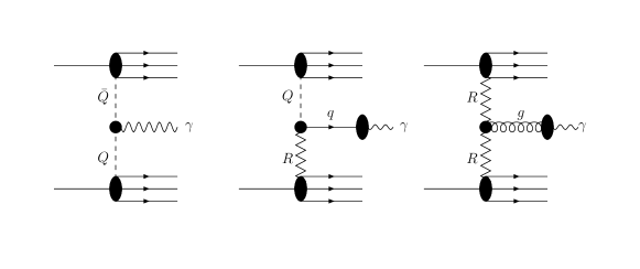
Figure 7: The mechanisms of prompt photon hadroproduction in the LO QMRK approach.

In this part we consider an inclusive production of isolated photons at the Fermilab Tevatron Collider, i.e. the processe $p\bar{p}\to\gamma X$. In the conventional collinear approximation it is assumed that at LO prompt photons are produced mainly via quark-gluon Compton scattering $(qg\to\gamma q$) or quark – antiquark annihilation $(q\bar{q}\to g\gamma)$. In the QMRK approach the LO contribution comes from the Reggeized quark – Reggeized antiquark annihilation via the effective vertices $C_{\bar{Q}Q}^{\gamma}$ (4). The additional small contributions originate from fragmentation of produced quarks and gluons into the photon, which is described by the parton to photon fragmentation functions $D_{q\to\gamma}(z,\mu^{2})$ and $D_{g\to\gamma}(z,\mu^{2})$ DukeOwens . The Fig. 7 schematically shows all relevant contributions to the isolated photon hadroproduction in the LO QMRK approach.

We start from the factorization formula, which connects the hadron $d\sigma(p\bar{p}\to\gamma X)$ cross section with the cross section of Reggeon’s collision $d\hat{\sigma}(Q\bar{Q}\to\gamma)$, and which is presented as follows

$$d\sigma(p\bar{p}\to\gamma X)=\sum_{q}\int\frac{dx_{1}}{x_{1}}\int\frac{d^{2}q_{1T}}{\pi}\int\frac{dx_{2}}{x_{2}}\int\frac{d^{2}q_{2T}}{\pi}\Phi_{q,\bar{q}}^{p}(x_{1},t_{1},\mu^{2})\Phi_{\bar{q},q}^{\bar{p}}(x_{2},t_{2},\mu^{2})d\hat{\sigma}(Q\bar{Q}\to\gamma),$$ (21)

where $\Phi_{q,\bar{q}}^{p,\bar{p}}(x_{1},t_{1},\mu^{2})$ is the Reggeized quark (anti-quark) unintegrated distribution function in a proton (anti-proton), $t_{1,2}=-q_{1,2T}^{2}$, $\mu=p_{T}$ is taken as the renormalization, factorization, and fragmentation scale, $p_{T}$ is the photon transverse momentum. In the case of photon production via the fragmentation we need to do a convolution with the relevant fragmentation function, for example in the following way

$$d\sigma(p\bar{p}\to\gamma X) = \sum_{q,\bar{q}}\int\frac{dx_{1}}{x_{1}}\int\frac{d^{2}q_{1T}}{\pi}\int\frac{dx_{2}}{x_{2}}\int\frac{d^{2}q_{2T}}{\pi}\int dz\times$$ (22)

$$\times \Phi_{q,g}^{p}(x_{1},t_{1},\mu^{2})\Phi_{g,q}^{\bar{p}}(x_{2},t_{2},\mu^{2})d\hat{\sigma}(QR\to q)D_{q\to\gamma}(z,\mu^{2}),$$

where $\Phi_{g}^{p,\bar{p}}(x_{1},t_{1},\mu^{2})$ is the Reggeized gluon unintegrated distribution function in a proton (anti-proton). In our calculations we use simple LO fragmentation functions $D_{q,g\to\gamma}(z,\mu^{2})$, which are taken from Ref.DukeOwens .

The transverse momentum $p_{T}$ spectra of isolated photon were studied by CDFCDF18 Collaboration and D0D018 ; D0196 Collaboration at the energies $\sqrt{S}=1.8$ TeV and $\sqrt{S}=1.96$ TeV. The inclusive prompt photon production cross section was measured in the range of $10\leq p_{T}\leq 300$ GeV, both in the central region, where the pseudorapidity is $|\eta|<0.9$, and in the forward region, where one takes on values in the range of $1.6<|\eta|<2.5$.

The master formula for the differential spectrum of the directly produced photon can be presented in the following way:

$$p_{T}^{3}\frac{d\sigma}{dp_{T}}(p\bar{p}\to\gamma X)=\sum_{q}\int d\eta\int d\phi_{1}\int dt_{1}\Phi_{q,\bar{q}}^{p}(x_{1},t_{1},\mu^{2})\Phi_{\bar{q},q}^{\bar{p}}(x_{2},t_{2},\mu^{2})\overline{|M(Q\bar{Q}\to\gamma|^{2}},$$ (23)

where $p_{0}=\frac{1}{2}p_{T}(e^{\eta}+e^{-\eta})$ is the photon energy, $p_{z}=\frac{1}{2}p_{T}(e^{\eta}-e^{-\eta})$ is the photon longitudinal momentum in respect of the proton beam, $\phi_{1}$ is the angle between ${\bf p}_{T}$ and ${\bf q}_{1T}$, and

$$x_{1}=\frac{p_{0}+p_{z}}{\sqrt{S}},\quad x_{2}=\frac{p_{0}-p_{z}}{\sqrt{S}},\quad t_{2}=t_{1}-2p_{T}\sqrt{t_{1}}\cos(\phi_{1})+p_{T}^{2},\quad p_{T}^{2}=x_{1}x_{2}S.$$

In the case of the photon production via a quark fragmentation the photon $p_{T}-$spectrum can be presented as follows

$$p_{T}^{3}\frac{d\sigma}{dp_{T}}(p\bar{p}\to\gamma X) = \sum_{q,\bar{q}}\int d\eta\int d\phi_{1}\int dt_{1}\int dz~{}\Phi_{q,g}^{p}(x_{1},t_{1},\mu^{2})\Phi_{g,q}^{\bar{p}}(x_{2},t_{2},\mu^{2})\times$$ (24)

$$\times z^{2}D_{q\to\gamma}(z,\mu^{2})\overline{|M(QR\to q|^{2}},$$

where

$$x_{1}=\frac{p_{0}+p_{z}}{\sqrt{S}z},\quad x_{2}=\frac{p_{0}-p_{z}}{\sqrt{S}z},\quad t_{2}=t_{1}-2\frac{p_{T}}{z}\sqrt{t_{1}}\cos(\phi_{1})+\frac{p_{T}^{2}}{z^{2}}.$$

In the Figures (8), (9) and (10) we present the results of our calculation in comparison with the D0 Collaboration data D018 ; D0196 at the energy $\sqrt{S}=1.8$ Tev and $\sqrt{S}=1.96$ TeV, correspondingly. We see that the agreement between the data and the theoretical calculation is well, especially in the central region of a pseudorapidity $|\eta|<0.9$. The contribution of the fragmentation production mechanism is very small at the $\sqrt{S}=1.8$ TeV and it is negligible at the energy $\sqrt{S}=1.96$ TeV. It is a very interesting fact, that at the energy $\sqrt{S}=1.96$ TeV we describe the data up to $p_{T}\simeq 300$ GeV. That directly demonstrates valid behavior and correct normalization of the quark unintegrated structure function $\Phi_{q}^{p}(x,t,\mu^{2})$, which is obtained using KMR prescription KMR , in the wide region of parameters $x$ and $t$.

V Discussion

In this section let us to compare our results with the previous studies of DIS and prompt photon production in the $k_{T}-$factorization approach, which were published in the Refs. WattMartinRyskin ; KMRgamma ; ZotovLipatovGamma ; SzczurekGamma recently.

The electron – quark DIS in the $k_{T}-$factorization approach was considered in the Ref. WattMartinRyskin . It was assumed that in DIS the transverse momentum of the off-shell quark much smaller than the photon virtuality ${\bf k}_{T}^{2}\ll Q^{2}$, and the $k_{T}-$dependence in the numerator of the relevant amplitude was ignored. In other words, in this approximation the conventional gamma-quark vertex was used, and gauge dependence of the off-shell amplitude was lost. It was obtained for the DIS structure functions WattMartinRyskin :

$$F_{2}(x_{B},Q^{2}) = \sum_{q,\bar{q}}e_{q}^{2}\int dt_{2}\left(\frac{x_{B}}{x_{2}}\right)\Phi_{q,\bar{q}}(x_{2},t_{2},\mu^{2}),$$ (25)

$$F_{L}(x_{B},Q^{2}) = 0.$$ (26)

The differences between our formulas (17)– (18) and ones (25) – (26), demonstrate that gauge invariance condition for amplitudes controls the correct $k_{T}-$dependence of the DIS structure functions. The formulas (25) and (26) don’t describe the experimental data at the LO and one needs the NLO contribution coming from the photon-gluon fusion subprocesses. The calculation of a cross section within the QMRK approach for the process under consideration

$$\gamma^{\star}+R\to q+\bar{q},$$ (27)

where $q$ is the massless quark, needs especial analysis with extraction of different singularities, see Ref. FadinIvanovKotsky for example. The calculation of DIS structure functions in the QMRK approach at the NLO has not been made up today. As it was shown above, even the LO approximation with the Reggeized quark describes data well, and this NLO contribution should be small.

The calculations of the inclusive prompt photon production at the Tevatron were performed using off-shell amplitudes involving initial quark in the Refs. KMRgamma ; ZotovLipatovGamma ; SzczurekGamma . In all these papers the LO contribution coming from the annihilation of a Reggeized quark and a Reggeized anti-quark ($Q+\bar{Q}\to\gamma$) was ignored and a Compton process of the off-shell quark – off-shell gluon scattering $g^{\star}+q^{\star}\to\gamma+q$ was considered as the LO process. We can’t explain this approximation. Evidently, if we work with off-shell initial quarks we need to take into account the process $q^{\star}+\bar{q}^{\star}\to\gamma$ as the LO approximation. We especially used here different denotations for the Reggeized particles ($Q,R$) and off-shell particles ($q^{\star},g^{\star}$). It means that in the Refs. KMRgamma ; ZotovLipatovGamma ; SzczurekGamma the conventional QCD vertices are used and the authors have obtained the gauge uninvariant amplitudes. The inclusion of the $k_{T}$-effects in the kinematics only without the using of the correct vertices for Reggeized particle interactions, can be considered as phenomenological trick, but such inclusion has not predictive power. The Compton scattering of Reggeized gluons on Reggeized quarks,

$$R+Q\to\gamma+q,$$ (28)

is a NLO QMRK process, when it is used to calculate inclusive photon production one needs to solve the same problems as for other NLO Reggeon-Reggeon to Particle-Particle processes in the QMRK approach. First of all, it is necessary to obtain the relevant effective vertices. This task have not been solved yet. Of course, the relevant process is LO if we study the associated photon plus jet, both with the larger transverse momenta, production.

VI Conclusion

We have shown that the quark Reggeization hypothesis is a very powerful tool in the high energy phenomenology for the hard processes involving quark exchanges. It is shown that it is possible to describe data at the LO QMRK approach for the DIS structure functions $F_{2}$ and $F_{L}$ of lepton – proton scattering, and prompt photon spectra for the inclusive production in the $p\bar{p}$ collisions at high energies. The scheme suggested in this paper is principally new in comparison with both the conventional collinear approximation and the $k_{T}-$factorization approach, which was developed earlier using Reggeized gluons only.

VII Acknowledgements

We thank L. Lipatov for the censorious remarks and useful discussion of the questions under consideration in this paper. We also thank D. Vasin and A. Shipilova for help in numerical calculations.

Figure 1: The $C_{Q\bar{Q}}^{g}$ effective vertices.

Figure 2: The $C_{\gamma Q}^{q}$ effective vertices.

Figure 3: $F_{2}(x_{B},Q^{2})$ and $F_{L}(x_{B},Q^{2})$ at $Q^{2}=12$ GeV². The data are from H1 Collaboration H1DIS .

Figure 4: $F_{2}(x_{B},Q^{2})$ and $F_{L}(x_{B},Q^{2})$ at $Q^{2}=25$ GeV². The data are from H1 Collaboration H1DIS .

Figure 5: $F_{2}(x_{B},Q^{2})$ and $F_{L}(x_{B},Q^{2})$ at $Q^{2}=60$ GeV² .The data are from H1 Collaboration H1DIS .

Figure 6: $F_{2}(x_{B},Q^{2})$ and $F_{L}(x_{B},Q^{2})$ at $Q^{2}=120$ GeV². The data are from H1 Collaboration H1DIS .

Figure 8: The $p_{T}-$spectrum of prompt photon at $\sqrt{S}=1.8$ TeV and $|\eta|<0.9$. The curve 1 is the direct production, 2 is the fragmentation production, 3 is their sum. The data are from D0 Collaboration D018 .

Figure 9: The $p_{T}-$spectrum of prompt photon at $\sqrt{S}=1.8$ TeV and $1.6<|\eta|<2.5$. The curves are the same as in Fig. 8. The data are from D0 Collaboration D018 .

Figure 10: The $p_{T}-$spectrum of prompt photon at $\sqrt{S}=1.96$ TeV and $|\eta|<0.9$ . The curves are the same as in Fig. 8. The data are from D0 Collaboration D0196 .

References

- (1) L. V. Gribov, E. M. Levin, and M. G. Ryskin, Phys. Rept. 100, 1 (1983).
- (2) J. C. Collins and R. K. Ellis, Nucl. Phys. B360, 3 (1991).
- (3) S. Catani, M. Ciafoloni, and F. Hautmann, Nucl. Phys. B366, 135 (1991).
- (4) V. S. Fadin and L. N. Lipatov, Nucl. Phys. B477, 767 (1996); Nucl. Phys. B406, 259 (1993).
- (5) B. A. Kniehl, V. A. Saleev, and D. V. Vasin, Phys. Rev. D 73, 074022 (2006); Phys. Rev. D 74, 014024 (2006); V. A. Saleev and D. V. Vasin, Phys. Rev. D 68, 114013 (2003); V. A. Saleev, Phys. Rev. D 65, 054041 (2002).
- (6) L. N. Lipatov, Nucl. Phys. B452, 369 (1995).
- (7) V. S. Fadin, M. I. Kotsky, and L. N. Lipatov, Phys. Lett. B 415, 97 (1997); D. Ostrovsky, Phys. Rev. D 62, 054028 (2000); V. S. Fadin, M. G. Kozlov, and A. V. Reznichenko. Report No. DESY 03-025 (2003); J. Bartels, A. S. Vera, and F. Schwennsen, JHEP 0611: 051 (2006).
- (8) V. S. Fadin and V. E. Sherman, JETP Lett. 23, 548 (1976); JETP 45, 861 (1977).
- (9) D0 Collaboration, B. Abbott et al., Phys. Rev. Lett. 84, 2786 (2000).
- (10) CDF Collaboration, D. Acosta et al., Phys. Rev. D 70, 074008 (2004).
- (11) D0 Collaboration, V. M. Abazov et al., Phys. Lett. B 639, 151 (2006).
- (12) M. A. Kimber, A. D. Martin, and M. G. Ryskin, Phys. Rev. D 63, 114027 (2001).
- (13) M. A. Kimber, A. D. Martin, and M. G. Ryskin, Eur. Phys. J. C 12, 655, (2000).
- (14) A. V. Lipatov and N. P. Zotov, Phys. Rev. D 72, 054002 (2005).
- (15) T. Pietrycki and A. Szczurek, Phys. Rev. D 75, 014023 (2007).
- (16) E. A. Kuraev, L. N. Lipatov, and V. S. Fadin, Sov. Phys. JETP 44, 443 (1976) [Zh. Eksp. Teor. Fiz. 71, 840 (1976)]; I. I. Balitsky and L. N. Lipatov, Sov. J. Nucl. Phys. 28, 822 (1978) [Yad. Fiz. 28, 1597 (1978)].
- (17) E. N. Antonov, L. N. Lipatov, E. A. Kuraev, and I. O. Cherednikov, Nucl. Phys. B 721, 111 (2005).
- (18) L. N. Lipatov and V. S. Fadin, JETP Lett. 49, 352 (1989); Sov. J. Nucl. Phys. 50, 712 (1989).
- (19) M. Gell-Mann, M. L. Goldberger, F. E. Low, E. Marx, and F. Zachariasen, Phys. Rev. 133, 145B (1964).
- (20) V. S. Fadin and R. Fiore, Phys. Rev. D 64, 114012 (2001).
- (21) A. V. Bogdan and V. S. Fadin, Nucl. Phys. B 740, 36 (2006).
- (22) G. Watt, A. D. Martin and M. G. Ryskin, Eur. Phys. J. C 31, 73 (2003); Phys. Rev. D 70, 014012 (2004).
- (23) H1 Collaboration, J. C. Adloff et al., Eur. Phys. J. C 21, 33 (2001).
- (24) D. W. Duke and J. F. Owens, Phys. Rev. D 26, 1600 (1982); J. F. Owens, Rev. Mod. Phys. 59, 465 (1987).
- (25) V. S. Fadin, D. Yu. Ivanov and M. I. Kotsky, Nucl. Phys. B 658, 156 (2003).