Coupling superconducting flux qubits at optimal point via dynamic decoupling from the quantum bus

Abstract

We propose a scheme with dc-control of finite bandwidth to implement two-qubit gate for superconducting flux qubits at the optimal point. We provide a detailed non-perturbative analysis on the dynamic evolution of the qubits interacting with a common quantum bus. An effective qubit-qubit coupling is induced while decoupling the quantum bus with proposed pulse sequences. The two-qubit gate is insensitive to the initial state of the quantum bus and applicable to non-perturbative coupling regime which enables rapid two-qubit operation. This scheme can be scaled up to multi-qubit coupling.

I Introduction

Superconducting Josephson junction (JJ) qubits (for a review, see e.g. Makhlin et al. (2001); You and Nori (2005); Wendin and Shumeiko (2006); Clarke and Wilhelm (2008)) provide an arena to study macroscopic quantum phenomena and act as promising candidates towards quantum information processing. For the three basic types of superconducting qubit, namely charge qubit, flux qubit and phase qubit, single qubit coherent operations with high quality factor have been demonstrated in many laboratories Nakamura et al. (1999); Vion et al. (2002); Yu et al. (2002); Martinis et al. (2002); Chiorescu et al. (2003); Saito et al. (2004); Johansson et al. (2006); Deppe et al. (2008). However, the best way to achieve controllable coupling and universal two-qubit gate are still open questions. A number of experimental attempts Pashkin et al. (2003); Yamamoto et al. (2003); Berkley et al. (2003); Johnson et al. (2003); Izmalkov et al. (2004); Xu et al. (2005); McDermott et al. (2005); Majer et al. (2005); Plourde et al. (2005); Hime et al. (2006); Harris et al. (2007); Ploeg et al. (2007); Niskanen et al. (2007); Plantenberg et al. (2007); Sillanpää et al. (2007); Majer et al. (2007) as well as theoretical proposals have been put forward Makhlin et al. (1999); You et al. (2002); Averin and Bruder (2003); Wang et al. (2004); Plourde et al. (2004); Rigetti et al. (2005); Liu et al. (2006); Bertet et al. (2006); Niskanen et al. (2006); Grajcar et al. (2006); Paraoanu (2006); Ashhab et al. (2006); Blais et al. (2007); Nakano et al. (2007) according to the characteristics of each specific circuit. In this paper, our discussion will be focused on coupling superconducting flux qubits Mooij et al. (1999); Orlando et al. (1999); Wilhelm and Semba (2006).

The straightforward consideration to realize two-qubit entanglement is utilizing the fixed inductive coupling between two flux qubits. With tunable single-qubit energy spacing, this fixed coupling can be used to demonstrate two-qubit logic gate Plantenberg et al. (2007). However, tunable coupling is required to achieve universal quantum computing. At early stage, dc-pulse control is widely adopted in the tunable coupling proposals You et al. (2005); Plourde et al. (2004). Main disadvantage for this method is the inefficiency to work at the degeneracy point which is a low-decoherence sweet spot. At the optimal point, the natural inductive coupling is off-diagonal in the diagonal representation of the free Hamiltonian. Hence the coupling only has second-order effect on the qubit dynamic for the detuned qubits. Another difficulty related with dc control is the operation error related to the finite rising-and-falling time of the dc-pulse. Recently, more attention is paid to coupling schemes with ac-pulse control Rigetti et al. (2005); Bertet et al. (2006); Liu et al. (2006); Niskanen et al. (2006); Ashhab et al. (2006); Niskanen et al. (2007). While most of the ac-control coupling schemes can work at the degeneracy point and no additional circuitry is needed Rigetti et al. (2005); Ashhab et al. (2006), some of them require strong driving Rigetti et al. (2005) or result in slow operation Ashhab et al. (2006). Meanwhile, unwanted crosstalk is present due to a always-on coupling. The possible solution to the above problems is the parametric coupling scheme with a tunable circuit acting as coupler Bertet et al. (2006). A third flux qubit has been demonstrated as a candidate for this coupler Niskanen et al. (2006, 2007). However incorporating additional nonlinear component to the circuit would increase the complexity of the circuit and might introduce additional noise and operation errors.

In this paper, we propose a scalable coupling mechanism of flux qubits with four Josephson junctions in two loops (4JJ-2L). The coupling is induced by a common quantum bus, such as a LC resonator or a one-dimensional superconducting transmission line resonator (TLR). The effective coupling Hamiltonian is diagonal with the free Hamiltonian of single qubit at the optimal point. With appropriate dc-control pulse, a dynamic two-qubit quantum gate can be realized for superconducting flux qubits at the optimal point. The on-and-off of the coupling can be switched by dc-pulse of finite bandwidth without introducing additional error. This protocol is based on the time evolution of a non-perturbative interaction Hamiltonian. Therefore it is applicable to ”ultra strong coupling” regime, where the coupling strength is comparable to qubit free Hamiltonian. Contrarily to parametric coupling which requires a strongly non-linear coupling element, the scheme described in this paper utilizes a linear element. The strong non-linearity of parametric coupler required in order to achieve fast enough two-qubit gates induces strong imperfections of the gates and added the difficulties related with microwave control Niskanen et al. (2006). While the two-qubit gate based on linear coupler is intrinsically free of errors if proper DC control is achieved. Thus the linearity of the coupler considered in this work has not only the advantage to be insensitive to the state of the coupler, but also offers the possibility of error-free gates. Due to these advantages, this new proposal could be a promising alternative in experiments.

This paper is organized as follows. In Sec. II, we first analyze the energy spectrum of the 4JJ-2L qubit configuration Mooij et al. (1999); Orlando et al. (1999). In Sec. III, the setup of our coupling mechanism for this type of qubit is described and the system Hamiltonian is derived. In Sec. IV, we present two different pulse sequences to realize the effective two-qubit coupling and construct two-qubit logic gates. The characteristics of this coupling scheme based on experimental consideration are analyzed in Sec. V. The discussions of this paper are given in Sec. VI.

II Flux qubit with tunable qubit gap

A single flux qubit discussed in this paper is shown in Fig. (1). Each qubit is composed of four Josephson junctions in two loops: the main loop (lower loop) and the dc SQUID loop (upper loop). The main loop encloses three junctions: two identical junctions with Josephson energy $E_{\text{J}}^{(i)}$ and one shared with the dc SQUID loop with Josephson energy $\alpha_{0}^{\left(i\right)}E_{\text{J}}^{\left(i\right)}$ where $\alpha_{0}^{(i)}$ is the ratio of the Josephson energy between the first two junctions and the third one (here and hereafter, the superscript $(i)$ denotes the variables of the $i$-th qubit). The main loop forms a flux qubit whose energy eigenstates are the superpositions of the clockwise and the counterclockwise persistent current states Mooij et al. (1999); Orlando et al. (1999). The 4-JJ flux qubit is different from the conventional design of a flux qubit due to the additional dc SQUID loop. The third junction of 3-JJ flux qubit is replaced by a dc SQUID in this 4-JJ design. Therefore the effective Josephson energy of the third junction can be controlled by the magnetic flux $\Phi_{\text{d}}^{\left(i\right)}$ threading the dc SQUID loop. Assuming the two junctions in the dc SQUID loop are identical, the effective Josephson energy is $\alpha^{(i)}(\Phi^{(i)}_{\text{d}})E_{\text{J}}^{(i)}\equiv 2\alpha_{0}^{\left(i\right)}\cos\left(\pi\Phi_{\text{d}}^{\left(i\right)}/\Phi_{0}\right)E_{\text{J}}^{(i)}$ with $\Phi_{0}$ the flux quantum. This feature, as we show later, enables the qubit gap to be tunable. This increases the in situ controllability of the quantum circuit Mooij et al. (1999); Orlando et al. (1999). The main loop and the dc SQUID loop of each qubit can be controlled by external on-site flux bias separately. A high-fidelity two-qubit operation has been proposed recently for the 4JJ-2L qubit Kerman (2008).

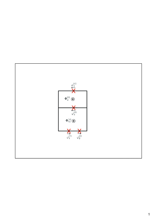
Figure 1: (Color online) The schematic of a single qubit with four Josephson junctions (denoted by cross) connected in two superconducting loops. The upper loop forms a dc SQUID with two identical junctions while the lower loop encloses three junctions similar as the conventional 3-JJ flux qubit. Each loop can be controlled separately by external magnetic flux $\Phi^{(i)}_{\text{d}}$ and $\Phi^{(i)}_{\text{m}}$ respectively.

As shown in Fig. (1), the Josephson phase differences of the four junctions in one qubit are denoted by $\varphi_{1}^{\left(i\right)}$, $\varphi_{2}^{\left(i\right)}$, $\varphi_{3}^{\left(i\right)}$ and $\varphi_{4}^{\left(i\right)}$ respectively. By defining $\tilde{\varphi}_{3}^{\left(i\right)}\equiv(\varphi_{3}^{\left(i\right)}+\varphi_{4}^{\left(i\right)})/2$, the total Josephson energy in one qubit loop is $-U_{0}^{\left(i\right)}=E_{\text{J}}^{\left(i\right)}\cos\varphi_{1}^{\left(i\right)}+E_{\text{J}}^{\left(i\right)}\cos\varphi_{2}^{\left(i\right)}+\alpha^{\left(i\right)}(\Phi_{\text{d}}^{\left(i\right)})E_{\text{J}}^{\left(i\right)}\cos\tilde{\varphi}_{3}^{\left(i\right)}$, where we have used the fluxoid quantization relation in the dc SQUID loop:

$$\varphi_{3}^{\left(i\right)}-\varphi_{4}^{\left(i\right)}=-2\pi\frac{\Phi_{\text{d}}^{\left(i\right)}}{\Phi_{0}}.$$ (1)

There are two other fluxoid quantization relations for this circuit:

$$\varphi_{1}^{\left(i\right)}+\varphi_{2}^{\left(i\right)}+\varphi_{3}^{\left(i\right)} = 2\pi\frac{\Phi_{\text{m}}^{\left(i\right)}}{\Phi_{0}},$$

$$\varphi_{1}^{\left(i\right)}+\varphi_{2}^{\left(i\right)}+\varphi_{4}^{\left(i\right)} = 2\pi\frac{\Phi_{\text{d}}^{\left(i\right)}+\Phi_{\text{m}}^{\left(i\right)}}{\Phi_{0}},$$ (2)

where $\Phi_{\text{m}}^{\left(i\right)}$ the magnetic flux threading the main qubit loop. Adding up the two equations in (2), we get

$$\varphi_{1}^{\left(i\right)}+\varphi_{2}^{\left(i\right)}+\tilde{\varphi}_{3}^{\left(i\right)}=2\pi\frac{\Phi_{\text{t}}^{\left(i\right)}}{\Phi_{0}},$$ (3)

where $\Phi_{\text{t}}^{\left(i\right)}\equiv\Phi_{\text{m}}^{\left(i\right)}+\Phi_{\text{d}}^{\left(i\right)}/2$ is the total magnetic flux threading the qubit loop. Then the total Josephson energy of the four junctions in the loop is

$$-U_{0}^{(i)} = \alpha^{\left(i\right)}(\Phi_{\text{d}}^{\left(i\right)})E_{\text{J}}^{(i)}\cos\left(2\pi\frac{\Phi_{\text{t}}^{\left(i\right)}}{\Phi_{0}}-\left(\varphi_{1}^{\left(i\right)}+\varphi_{2}^{\left(i\right)}\right)\right)$$ (4)

$$+E_{\text{J}}^{(i)}\cos\varphi_{1}^{\left(i\right)}+E_{\text{J}}^{(i)}\cos\varphi_{2}^{\left(i\right)}.$$

It takes the same form as that of the 3-JJ flux qubit Mooij et al. (1999); Orlando et al. (1999) except that the ratio $\alpha^{\left(i\right)}$ is tunable. If the total magnetic flux $\Phi_{\text{t}}^{\left(i\right)}$ is close to half a flux quantum $\Phi_{0}/2$ and $\alpha^{(i)}>0.5$, the function $U_{0}\left(\varphi_{1}^{\left(i\right)},\varphi_{2}^{\left(i\right)}\right)$ represents a landscape with periodic double-well potentials.

With external flux bias, one can set the operation point in one double-well potential. The classical stable states of this potential correspond to the clockwise and the counter-clockwise persistent current states. By changing the ratio $\alpha^{\left(i\right)}$ between the Josephson energy of the third junction (through the dc SQUID), the height of the tunneling barrier (hence the tunneling rate) between the two minima of each double-well is tunable. When $\alpha^{\left(i\right)}$ is set in appropriate range, coherent tunneling between the two wells of the potential is enabled while the tunneling between different potentials is highly suppressed.

Taking into account the electric energy stored in the four capacitors, we can get the full Hamiltonian of this system. The energy spectrum of the circuit with $\alpha^{\left(i\right)}=0.8$ and $E_{\text{J}}^{(i)}/E_{\text{C}}^{(i)}=35$ ($E_{\text{C}}^{(i)}=e^{2}/2C$ denotes the Coulomb energy of the first (second) junction of the $i$-th qubit and $C$ is the junction capacitance) is shown in Fig. 2 as a function of the rescaled total magnetic flux $f^{\left(i\right)}=\Phi_{\text{t}}^{\left(i\right)}/\Phi_{0}$.

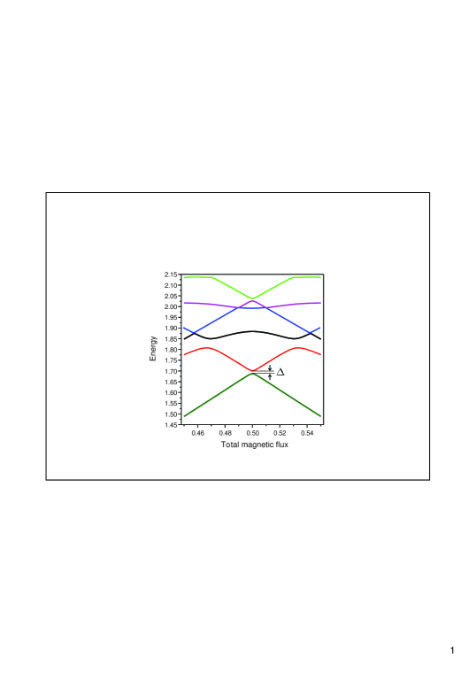
Figure 2: (Color online) The energy spectrum of the lowest six energy levels of the superconducting loop with respect to the total magnetic flux $\Phi_{\text{t}}^{(i)}$. The energy is in the unit of $E_{\text{J}}$ while the magnetic flux is in the unit of $\Phi_{0}$. We take $E_{\text{J}}^{(i)}/E_{\text{C}}^{(i)}=35$ and $\alpha^{(i)}=0.8$.

In the vicinity of $\Phi_{\text{t}}^{\left(i\right)}=\Phi_{0}/2$, the lowest two energy levels are far away from other energy levels and form a two-level subspace which can be used as a flux qubit. The eigenstates of the flux qubit are superpositions of the clockwise and the counter-clockwise persistent current states. The 4-JJ flux qubit works the same as its 3-JJ prototype except that the barrier height of the double-well potential is tunable in situ. In the two-level subspace, the free Hamiltonian for the $i$-th qubit is written as

$$H^{\left(i\right)}=\frac{\varepsilon^{\left(i\right)}(\Phi_{\text{t}}^{\left(i\right)})}{2}\sigma_{{z}}^{\left(i\right)}+\frac{\Delta^{\left(i\right)}(\Phi_{\text{d}}^{\left(i\right)})}{2}\sigma_{x}^{\left(i\right)}$$ (5)

where $\varepsilon^{\left(i\right)}$ is the energy spacing of the two classical current states

$$\varepsilon^{\left(i\right)}(\Phi_{\text{t}}^{\left(i\right)})\approx 2I_{p}^{\left(i\right)}\left(\Phi_{\text{t}}^{\left(i\right)}-\frac{\Phi_{0}}{2}\right)$$ (6)

and $\Delta^{\left(i\right)}$ is the energy gap between the two states at the degeneracy point $\Phi_{\text{t}}^{(i)}=\Phi_{0}/2$,

$$\Delta^{\left(i\right)}(\Phi_{\text{d}}^{\left(i\right)})\equiv\Delta^{\left(i\right)}(\alpha^{\left(i\right)}=2\alpha_{0}^{\left(i\right)}\cos(\pi\frac{\Phi_{\text{d}}^{\left(i\right)}}{\Phi_{0}})).$$ (7)

According to the tight-binding model, $\Delta^{(i)}$ can be evaluated through WKB approximation Orlando et al. (1999) as $\Delta^{(i)}\approx(\omega_{a}/2\pi)\exp(-[4\alpha(1+2\alpha)E_{\text{J}}^{(i)}/E_{\text{C}}^{(i)}]^{1/2}(\sin\phi^{*(i)}-\phi^{*(i)}/2\alpha))$ where $\omega_{a}$ is the attempt frequency of escape in the potential well and $\cos\phi^{*(i)}=0.5\alpha^{(i)}$ (the Planck constant $\hbar$ is set to be $1$). In Fig. 3, the energy gap $\Delta^{(i)}$ and its derivative $d\Delta^{(i)}/d\alpha^{\left(i\right)}$ are shown as a function of $\alpha^{\left(i\right)}$. The results are obtained from numerical calculation and analytical derivation based on WKB approximation.

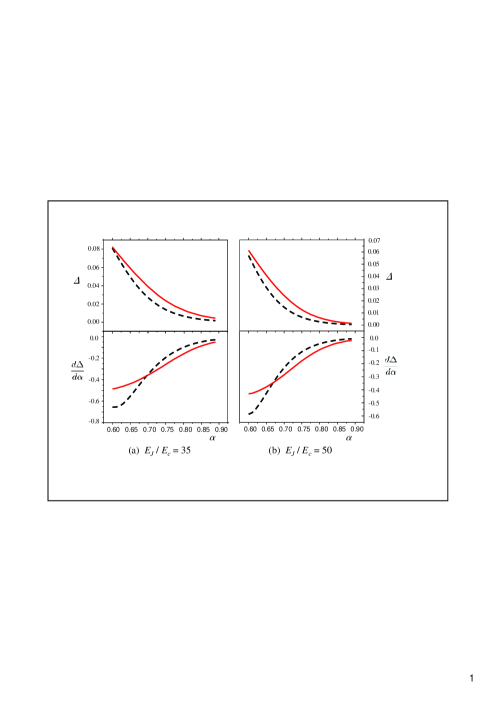
Figure 3: (Color online) The energy gap of single qubit $\Delta^{(i)}$ and its derivative $d\Delta^{(i)}/d\alpha^{\left(i\right)}$ as a function of $\alpha^{\left(i\right)}$ for (a) $E_{\text{J}}^{(i)}/E_{\text{C}}^{(i)}=35$ and (b) $E_{\text{J}}^{(i)}/E_{\text{C}}^{(i)}=50$ (for simplicity, the superscript $(i)$ is omitted in the figure). The solid line (red) is obtained from the exact diagonalization of the original 4-JJ qubit Hamiltonian while the dashed line (black) is obtained from the analytical solution of the tight-binding model with WKB approximation which breaks down at low barrier regime. The energy is in the unit of $E_{\text{J}}$.

III The Coupled System

A schematic to illustrate our coupling mechanism is shown in Fig. 4 with two different types of data bus, i.e., LC resonator and 1D TLR. For simplicity, we first concentrate on coupling two qubits. The problem of scale-up will be discussed later. As we described in the previous section, each qubit is composed of four Josephson junctions in two loops: the main loop (the lower loop) and the dc SQUID loop (the upper one). The main loop and the dc SQUID loop of each qubit can be controlled by external on-site flux bias independently. The two qubits are placed in sufficient distance so that the direct coupling can be effectively neglected Niskanen et al. (2007). The two qubits are both coupled with a common data bus such as a twisted LC resonator or 1D on-the-top TLR via mutual inductance.

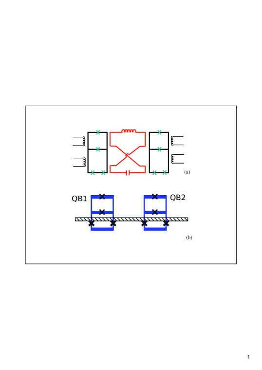
Figure 4: (Color online) The circuit design examples to implement the required coupling. Two 4JJ-2L flux qubits are coupled with each other through the inductive coupling with a resonator as data bus: (a) a twisted LC resonator and (b) a 1D superconducting transmission line resonator in a separate layer. The current of the data bus induces magnetic fluxes both in the upper loop and in the lower loop of each qubit. The directions of two magnetic fluxes are opposite.

Due to the mutual inductance with the resonator, the magnetic fluxes include the contribution both from the external applied flux and the resonator, i.e., $\Phi_{\text{m}}^{\left(i\right)}=\Phi_{\text{m,e}}^{\left(i\right)}+\Phi_{\text{m,b}}^{\left(i\right)}$ and $\Phi_{\text{d}}^{\left(i\right)}=\Phi_{\text{d,e}}^{\left(i\right)}+\Phi_{\text{d,b}}^{\left(i\right)}$, where the subscript $e(b)$ indicates the contribution from the external magnetic flux (the quantum data bus) respectively. Then the total magnetic flux $\Phi_{\text{t}}^{\left(i\right)}$ reads

$$\Phi_{\text{t}}^{\left(i\right)}=\left(\Phi_{\text{m,e}}^{\left(i\right)}+\frac{\Phi_{\text{d,e}}^{\left(i\right)}}{2}\right)+\left(\Phi_{\text{m,b}}^{\left(i\right)}+\frac{\Phi_{\text{d,b}}^{\left(i\right)}}{2}\right).$$ (8)

The coupling between a single qubit and the data bus includes two parts: the coupling of the qubit with the dc SQUID loop via mutual inductance $M_{\text{d}}^{\left(i\right)}$ and the coupling of the qubit with the main loop via $M_{\text{m}}^{\left(i\right)}$. The magnetic flux induced in the dc SQUID loop and the qubit main loop are

$$\Phi_{\text{d,b}}^{\left(i\right)} = M_{\text{d}}^{\left(i\right)}I$$

$$\Phi_{\text{m,b}}^{\left(i\right)} = M_{\text{m}}^{\left(i\right)}I$$ (9)

respectively and $I$ is the current in the resonator. For our purpose, the two magnetic fluxes satisfy

$$\Phi_{\text{d,b}}^{\left(i\right)}=-2\Phi_{\text{m,b}}^{\left(i\right)}.$$ (10)

This can be implemented by designing the mutual inductance

$$M_{\text{d}}^{\left(i\right)}=-2M_{\text{m}}^{\left(i\right)},$$ (11)

The minus in (10) is due to the special layout of the data bus so that the directions of the magnetic flux induced by the quantum bus in the upper loop and the lower loop are opposite. Inserting Eq. (10) into Eq. (8), we find the total flux $\Phi_{\text{t}}^{\left(i\right)}$ is contributed only by the external applied magnetic flux as $\Phi_{\text{t}}^{\left(i\right)}=\Phi_{\text{q,e}}^{\left(i\right)}+\Phi_{\text{d,e}}^{\left(i\right)}/2$. Since the $\sigma_{z}$ component of the qubit is coupled with $\Phi_{\text{t}}^{\left(i\right)}$, the resonator contributes a pure $\sigma_{x}$ coupling with no $\sigma_{z}$ component. Therefore the qubit can always be biased at the optimal point $\Phi_{\text{t}}^{(i)}=\Phi_{0}/2$.

For the quantized mode of the resonator,

$$I=\sqrt{\frac{\omega}{2L}}\left(a+a^{{\dagger}}\right).$$ (12)

where $\omega=(LC)^{-1/2}$ is the plasma frequency of resonator, $L$ ($C$) the lumped or distributed inductance (capacitance) of the resonator and $a^{{\dagger}}$ ($a$) the plasmon creation (annihilation) operator. With these denotations,

$$\Phi_{\text{d,b}}^{\left(i\right)}=f_{\text{d}}^{\left(i\right)}\left(a+a^{{\dagger}}\right)$$ (13)

where

$$f_{\text{d}}^{\left(i\right)}\equiv M_{\text{d}}^{\left(i\right)}\sqrt{\frac{\omega}{2L}}.$$ (14)

Usually the mutual inductance of the resonator and the qubit loop is about several pH to several tens of pH. For example, if we take $M_{\text{d}}^{\left(i\right)}=10$ pH, $\omega=1$ GHz and $L=100$ pH, $f_{\text{d}}^{\left(i\right)}/\Phi_{0}\approx 5.6\times 10^{-4}\ll 1$. This means the magnetic flux contributed from the resonator is much smaller than that from the external applied magnetic field. To the first order, the energy gap of a single qubit is modified by the resonator as

$$\Delta\left(\alpha^{\left(i\right)}\right)\approx\Delta\left(\alpha_{e}^{\left(i\right)}\right)-\left.\frac{d\Delta\left(\alpha^{\left(i\right)}\right)}{d\alpha^{\left(i\right)}}\right|_{\alpha^{\left(i\right)}=\alpha_{e}^{\left(i\right)}}\delta\alpha^{\left(i\right)}(a+a^{{\dagger}})$$ (15)

with

$$\alpha_{e}^{\left(i\right)} = 2\alpha_{0}^{\left(i\right)}\cos\left(\pi\frac{\Phi_{\text{d,e}}^{\left(i\right)}}{\Phi_{0}}\right)$$

$$\delta\alpha^{\left(i\right)} = 2\alpha_{0}^{\left(i\right)}\pi\sin\left(\pi\frac{\Phi_{\text{d,e}}^{\left(i\right)}}{\Phi_{0}}\right)\frac{f_{\text{d}}^{\left(i\right)}}{\Phi_{0}}$$ (16)

The Hamiltonian for a single qubit linearly interacting with the data bus reads,

$$H^{\left(i\right)} = \frac{\varepsilon^{\left(i\right)}\left(\Phi_{m,e}^{\left(i\right)}+\Phi_{\text{d,e}}^{\left(i\right)}/2\right)}{2}\sigma_{z}^{\left(i\right)}+\frac{\Delta^{\left(i\right)}\left(\Phi_{\text{d,e}}^{\left(i\right)}\right)}{2}\sigma_{x}^{\left(i\right)}$$ (17)

$$+g^{\left(i\right)}\left(\Phi_{\text{d,e}}^{\left(i\right)}\right)\sigma_{x}^{\left(i\right)}\left(a+a^{{\dagger}}\right)$$

with

$$\Delta^{\left(i\right)}\left(\Phi_{\text{d,e}}^{\left(i\right)}\right)\equiv\Delta\left(\alpha_{e}^{\left(i\right)}\right),$$ (18)

and the coupling coefficient

$$g^{\left(i\right)}\left(\Phi_{\text{d,e}}^{\left(i\right)}\right)\equiv\kappa^{\left(i\right)}\left(\Phi_{\text{d,e}}^{\left(i\right)}\right)\sqrt{\omega},$$ (19)

with

$$\kappa^{\left(i\right)}\left(\Phi_{\text{d,e}}^{\left(i\right)}\right)=-\left.\frac{d\Delta\left(\alpha^{\left(i\right)}\right)}{d\alpha^{\left(i\right)}}\right|_{\alpha^{\left(i\right)}=\alpha_{e}^{\left(i\right)}}\delta\alpha^{\left(i\right)}.$$ (20)

Note that magnitude of the coupling $g^{(i)}$ increases with the mutual inductance $M_{\text{d}^{(i)}}$. If $\Phi_{m,e}^{\left(i\right)}+\Phi_{\text{d,e}}^{\left(i\right)}/2=(n+0.5)\Phi_{0}$ (where $n=0,\pm 1,\pm 2$ is an arbitrary integer), qubit is biased at the degeneracy point and the system Hamiltonian is written as

$$H=\omega a^{{\dagger}}a+\sum_{i=1,2}\left(\frac{\Delta^{\left(i\right)}(\Phi_{\text{d,e}}^{\left(i\right)})}{2}\sigma_{x}^{\left(i\right)}+g^{\left(i\right)}(\Phi_{\text{d,e}}^{\left(i\right)})\sigma_{x}^{\left(i\right)}\left(a+a^{{\dagger}}\right)\right).$$ (21)

By tuning the external magnetic flux $\Phi_{\text{d,e}}^{\left(i\right)}$ in the dc SQUID loop to be$\ n\Phi_{0}$, $g^{\left(i\right)}(\Phi_{\text{d,e}}^{\left(i\right)})=0$, the qubit is decoupled from the resonator in the first order. The qubits act independently and single-qubit operation can be implemented by biasing $\Phi_{\text{q,e}}^{\left(i\right)}$ together with microwave pulse.

In the above discussion, the condition Eq. (11) is assumed. However it might not be precisely satisfied in practical case. Suppose there is a small deviation in the fabrication process that $M_{\text{d}}^{\left(i\right)}=-2(1+\delta)M_{\text{m}}^{(i)}$ (where $\delta\ll 1$), the total magnetic flux $\Phi_{\text{t}}^{\left(i\right)}$ includes a small contribution from the resonator,

$$\Phi_{\text{t}}^{\left(i\right)}=\Phi_{\text{q,e}}^{\left(i\right)}+\frac{\Phi_{\text{d,e}}^{\left(i\right)}}{2}-\delta M_{\text{m}}^{\left(i\right)}I.$$ (22)

This adds a term to the Hamiltonian Eq. (21): $g^{\prime\left(i\right)}\sigma_{z}^{\left(i\right)}\left(a+a^{{\dagger}}\right)$ with $g^{\prime\left(i\right)}=-\delta M_{\text{m}}^{\left(i\right)}I_{p}\sqrt{{\omega}/{2L}}$. However since the qubit is far-detuned (e.g. according to the parameters used in Sec. V, $\Delta\approx 15.28$ GHz and $\omega\approx 1$ GHz), this last term is a fast-rotating one and has negligible contribution. In the following, we adopt Eq. (21) as the effective system Hamiltonian.

IV The strategy to achieve effective two-qubit interaction

In this section, we discuss about how to achieve the two-qubit coupling in this composite system. The qubits only interact with each other indirectly through a common quantum bus. In the dispersive limit, the operation time of two-qubit logic gate is limited by the small ratio $g/{\delta\omega}$ where $g$ is the qubit-bus coupling and $\delta\omega$ the qubit-resonator detuning. In this case, the resonator is only virtually excited. In this paper we rely on another stradegy that the quantum bus carries real excitations. The effective two-qubit coupling is achieved by one or a series of specific unitary evolutions of the resonator-qubit composite system. Similar method has been discussed in the context of quantum computing with thermal ion-trap Milburn (1999); Sørensen and Mølmer (1999, 2000); Wang et al. (2001) and Josephson charge qubit Wang et al. (2004). The feature of this coupling is the insensitivity to the quantum state of the resonator. In ion-trap quantum computing, it is known as Sørenson-Mølmer gate and has been experimentally demonstrated Sackett et al. (2000); Leibfried et al. (2003); Haljan2005; Home et al. (2006). However, the original Sørenson-Mølmer relies on virtual excitations of the vibrational modes, whereas here the quantum bus carries real excitations.

If a dc-pulse is applied to $\Phi_{\text{d,e}}^{(i)}$ to shift it from $n\Phi_{0}$, the time evolution of the composite system is driven by the Hamiltonian Eq. (21). The operators included in the interaction Hamiltonian $(a+a^{{\dagger}})\sigma_{x}^{(i)}$ and the free Hamiltonian ($a+a^{{\dagger}}$, $\sigma_{x}^{(i)}$) may be enlarged by their commutator into a closed Lie algebra of finite dimension. Thus the exact solution of the time evolution can be decomposed into a product over exponentials of the generators Wei and Norman (1963). In the interaction picture,

$$H_{I}=\sum_{i}g^{\left(i\right)}\left(a^{{\dagger}}e^{i\omega t}+ae^{-i\omega t}\right)\sigma_{x}^{\left(i\right)}.$$ (23)

The corresponding closed Lie algebra is $\left\{a\sigma_{x}^{\left(i\right)},a^{{\dagger}}\sigma_{x}^{\left(i\right)},\sigma_{x}^{\left(1\right)}\sigma_{x}^{\left(2\right)},1\right\}$. The time evolution operator as the product of their exponentials can be written as

$$U_{\text{I}}(t) = e^{-iD\left(t\right)}e^{-iA(t)\sigma_{x1}\sigma_{x2}}\cdot$$ (24)

$$\left(\prod\limits_{i=1,2}e^{-iB_{i}(t)a\sigma_{x}^{\left(i\right)}}\right)\left(\prod\limits_{i=1,2}e^{-iB_{i}^{\ast}(t)a^{{\dagger}}\sigma_{x}^{\left(i\right)}}\right),$$

where

$$\left\{\begin{array}[]{c}B_{i}(t)=\frac{g^{\left(i\right)}}{-i\omega}\left(e^{-i\omega t}-1\right),\\ A\left(t\right)=\frac{2g^{\left(1\right)}g^{\left(2\right)}}{\omega}\left(\frac{1}{i\omega}\left(e^{i\omega t}-1\right)-t\right),\\ D\left(t\right)=\frac{(g^{\left(1\right)})^{2}+(g^{(2)})^{2}}{\omega}\left(\frac{1}{i\omega}\left(e^{i\omega t}-1\right)-t\right).\end{array}\right.$$ (25)

In the following discussion, we neglect the universal phase factor $D\left(t\right)$. If the last factor of Eq. (24) can be effectively canceled,

$$U_{\text{I}}\left(t\right)\equiv\exp[-iD\left(t\right)-iA(t)\sigma_{x1}\sigma_{x2}],$$ (26)

which represents the time evolution which is effectively governed by Hamiltonian $\sim\sigma_{x1}\sigma_{x2}$. This can be done in two different ways as described below:

Figure 5: (Color online) Schematics of the pulse sequence to realize two-qubit gate operation.

IV.1 Single pulse operation

By controlling the pulse length, a two-qubit gate is realized with a single dc-pulse which shifts $\Phi_{\text{d,e}}^{(i)}$ from $n\Phi_{0}$ (Fig. 5 (a)). While the whole time evolution Eq. (24) is non-periodic, Eq. (25) shows that $B_{i}(t)$ is a periodic function of time and it vanishes at $T_{n}={2n\pi}/{\omega}$. At these times, the time evolution operator in the interaction picture reduces to

$$U_{\text{I}}\left(T_{n}\right)=\exp\left(i4n\pi\kappa^{\left(1\right)}\kappa^{\left(2\right)}\sigma_{x1}\sigma_{x2}\right).$$ (27)

This is equivalent to a system of two coupled qubits with an interaction Hamiltonian $\propto\sigma_{x1}\sigma_{x2}$.

The minimum time to realize a rotation $U_{xx}(\theta)=\exp\left(i\theta\sigma_{x1}\sigma_{x2}\right)$ is

$$T_{\min}\equiv T_{m_{0}}=2m_{0}\pi/\omega$$ (28)

with

$$m_{0}=\left[n_{0}\right]=\left[\frac{\theta\omega}{4\pi\kappa^{\left(1\right)}\kappa{\left(2\right)}}\right],$$ (29)

where $\left[...\right]$ represents the integer part of a number. Note that we can not achieve a two-qubit rotation precisely unless $n_{0}$ happens to be an integer, so that $n_{0}=m_{0}$. The error of one two-qubit gate is of the order of $4\pi\kappa^{\left(1\right)}\kappa^{\left(2\right)}/\omega$ (about $1\%$ using practical parameters). This operation error can be avoided using a double-pulse method discussed below. It is notable that increasing the frequency of the resonator $\omega$ cannot achieve a faster two-qubit gate (due to the $\sqrt{\omega}$ dependence of $g^{\left(i\right)}$), but it can reduce the error of the two qubit gate.

IV.2 Double pulse operation

Alternatively a two-qubit logic operation can be constructed with two successive operations as shown in Fig. 5(b).

Initially $\Phi_{\text{d,e}}^{(i)}$ is biased at $n\Phi_{0}$. The first dc-pulse shifts it to a certain $\Phi_{\text{d,e}}^{(i)}\neq n\Phi_{0}$ for a duration ${t}/{2}$. The evolution operator (in the interaction picture) is $U_{\text{I}}\left(\frac{t}{2}\right)$. After time $t/{2}$, one reverses the direction of the magnetic flux in the dc SQUID loop so that $\Phi_{\text{d,e}}^{\left(i\right)}$ is changed into $-\Phi_{\text{d,e}}^{\left(i\right)}$ and $g^{\prime\left(i\right)}=-g^{\left(i\right)}$. The system is then driven by a new Hamiltonian $H^{\prime}=H\left(-g^{\left(i\right)}\right)$ for another ${t}/{2}$. The time evolution during the second pulse is

$$U_{I}^{{}^{\prime}}\left(t\right) = e^{-iD^{{}^{\prime}}\left(t\right)}e^{-iA^{{}^{\prime}}(t)\sigma_{x1}\sigma_{x2}}\cdot$$

$$\left(\prod\limits_{i=1,2}e^{-iB_{i}^{\ast^{\prime}}(t)a^{{\dagger}}\sigma_{xi}}\right)\left(\prod\limits_{i=1,2}e^{-iB_{i}^{{}^{\prime}}(t)a\sigma_{xi}}\right)$$

with

$$\left\{\begin{array}[]{c}B_{i}^{{}^{\prime}}(t)=-B_{i}(t)\\ A^{{}^{\prime}}\left(t\right)=\frac{2g_{1}g_{2}}{\omega}\left(\frac{1}{-i\omega}\left(e^{-i\omega t}-1\right)-t\right)\\ D^{{}^{\prime}}\left(t\right)=\frac{g_{1}^{2}+g_{2}^{2}}{\omega}\left(\frac{1}{-i\omega}\left(e^{-i\omega t}-1\right)-t\right)\end{array}\right.$$ (31)

Note that the two terms in the brackets of Eq. (LABEL:u4) are permuted comparing with Eq. (24), so that the expressions $A^{\prime}(t)$, $D^{\prime}(t)$ are different from $A(t)$, $D(t)$ in Eq. (25).

The dynamics for the above two consecutive steps is

$$U_{\text{tot}}\left(t\right) = U_{I}^{\prime}\left(\frac{t}{2}\right)U_{I}\left(\frac{t}{2}\right)$$ (32)

$$= \exp[-iM(t)\sigma_{x1}\sigma_{x2}]\exp[-iN\left(t\right)],$$ (33)

where

$$M(t) = \frac{2g^{\left(1\right)}g^{\left(2\right)}}{\omega}\left(\frac{2}{\omega}\sin\frac{\omega t}{2}-t\right),$$

$$N(t) = \frac{(g^{\left(1\right)})^{2}+(g^{(2)})^{2}}{\omega}\left(\frac{2}{\omega}\sin\frac{\omega t}{2}-t\right).$$ (34)

Therefore, the total time evolution is equivalent to the time evolution governed by two-qubit interaction $\sim\sigma_{x}^{\left(1\right)}\sigma_{x}^{\left(2\right)}$ together with a universal phase factor.

The time $T$ to realize a rotation $U_{xx}(\theta)$ in this way satisfies the nonlinear equation

$$\frac{\omega T}{2}-\sin\frac{\omega T}{2}=\frac{\theta\omega}{4\kappa^{\left(1\right)}\kappa^{\left(2\right)}}.$$ (35)

In the case of $\omega\gg g^{\left(i\right)}$, the solution is written as

$$T\approx\frac{\theta}{2\kappa^{\left(1\right)}\kappa^{\left(2\right)}}.$$ (36)

The two-qubit operation time is estimated using experimental parameters. Assuming $M_{\text{d}}=10$ pH and $L=100$ pH, one gets $g^{\left(i\right)}\approx 36.02\text{ MHz}$. As a cost of the low fluctuation related to the dc SQUID loop, the coupling strength associated with the dc SQUID loop is weaker than that with the main loop. For example, to realize a $U_{xx}\left(\frac{\pi}{2}\right)$, the operation time is about $204$ ns. It is smaller than the qubit coherence time at the optimal point. The operation time is proportional to $L/M_{\text{d}}^{2}$. Increasing the mutual inductance between the dc SQUID and the resonator reduces the operation time. It is worth to point out that the ratio $g/\omega$ is not required to be small. Therefore there is no fundamental limit on the operation time except the realizable coupling strength.

As discussed in Sec. III, arbitrary single qubit gate can be performed after switching off the qubit-bus interaction. Any non-trivial two-qubit gate can be built up with this xx coupling plus single qubit gates. For example, the C-phase gate can be constructed as (up to a global phase factor) Makhlin et al. (2001)

$$R\left(\theta\right)\equiv U_{z}^{\left(1\right)}\left(-\frac{\theta}{2}\right)U_{z}^{\left(2\right)}\left(-\frac{\theta}{2}\right)\exp\left(i\theta\tilde{\sigma}_{z}^{\left(1\right)}\tilde{\sigma}_{z}^{\left(2\right)}/4\right)$$ (37)

with $U_{z}^{\left(i\right)}\left(\theta\right)\equiv\exp\left(i\theta\tilde{\sigma}_{z}^{\left(i\right)}/2\right)=\exp\left(i\theta\sigma_{x}^{\left(i\right)}/2\right)$. Here we change representation so that $\tilde{\sigma}_{z}=\sigma_{x}$ and $\tilde{\sigma}_{x}=-\sigma_{z}$. And the CNOT gate can be readily constructed with C-phase gate as

$$\text{CNOT}=H^{\left(2\right)}R\left(\pi\right)H^{\left(2\right)},$$ (38)

where $H^{(i)}$ denote the Hadamard transformation on the $i$-th qubit as $H^{\left(i\right)}\equiv\exp\left(-i\pi\left(\sigma_{x}^{\left(i\right)}+\sigma_{z}^{\left(i\right)}\right)/2\sqrt{2}\right)$ (up to a phase factor).

With arbitrary single-qubit rotation and any non-trivial two-qubit rotation, universal quantum computing can be realized according to quantum network theorem Barenco et al. (1995).

V The features of this coupling protocol

In the previous section, we have presented the way to realize two-qubit coupling and logic gate with our proposed setup. In this section, the features of this coupling protocol are analyzed with emphasis on the experimental implementation. The qubit-qubit effective coupling commutes with the free Hamiltonian of the single qubit. This feature enables many practical advantages:

(1) The main idea to implement a two-qubit operation from the exact evolution operator Eq. (24) is to cancel the part related with the degree of freedom of the resonator, so that the final operation Eq. (26) represents a qubit-qubit operation without entanglement with resonator mode. Therefore the resonator mode does not transfer population with the qubit although the resonator mode mediates the qubit-qubit interaction. As a result, this two-qubit logic gate is insensitive to the initial state of the resonator Sørensen and Mølmer (1999). This feature is important for the experiment performed at finite temperature because the equilibrium state of the resonator is a mixed state. For example, there is $16\%$ population at the excited state for a $1$ GHz resonator at $30$ mK.

(2) As we mentioned, our coupling protocol works at the low-decoherence optimal point where the qubit is robust to flux fluctuation and has long decoherence time. This is in contrast to other coupling protocols with dc-pulse control You et al. (2005); Plourde et al. (2004). During the two-qubit operation, the control parameter is not the total magnetic flux but rather a component in the dc SQUID loop. Therefore, the qubit can be biased at the optimal point $\Phi_{\text{t}}^{\left(i\right)}=(n+1/2)\Phi_{0}$ during two-qubit operation.

While the dc SQUID adds a second control to the circuit, it introduces extra decoherence. The fluctuation of the flux threading the dc SQUID loop results in the fluctuation of the energy splitting $\Delta$ and introduces decoherence to the qubit dynamics. Suppose the magnetic flux are perturbed by the same amount of fluctuation as $\Phi_{\text{t}}^{(i)}\rightarrow\Phi_{\text{t}}^{(i)}+\delta\Phi$, $\Phi_{\text{d}}^{(i)}\rightarrow\Phi_{\text{d}}^{(i)}+\delta\Phi$. Therefore the first-order effect of the fluctuation of magnetic flux in the main loop and the sub-loop are $\delta E_{\text{t}}^{(i)}\equiv c_{\text{t}}^{(i)}\delta\Phi$ and $\delta E_{\text{d}}^{(i)}\equiv c_{\text{d}}^{(i)}\delta\Phi$ respectively, with $c_{\text{t}}^{(i)}\equiv\left|\partial E^{(i)}/\partial\Phi_{\text{t}}^{(i)}\right|$ and $c_{\text{d}}^{(i)}\equiv\left|\partial E^{(i)}/\partial\Phi_{\text{d}}^{(i)}\right|$, where $E^{(i)}$ is the energy level spacing of the qubit, $E^{(i)}=\sqrt{\varepsilon^{2}\left(\Phi_{\text{t}}^{(i)}\right)+\Delta^{2}\left(\Phi_{\text{d}}^{(i)}\right)}$. If a qubit Chiorescu et al. (2003) with $E_{\text{J}}/\hbar=259$ GHz, $E_{\text{J}}/E_{c}=35$ and $2\alpha_{0}=0.8$ is biased at $\Phi_{\text{t}}=\Phi_{0}/2$ and $2\alpha_{0}\cos\left(\pi\Phi_{\text{d}}/\Phi_{0}\right)\approx 0.65$, we get

$$c_{\text{d}}^{(i)}=163\text{ GHz}/\Phi_{0}.$$ (39)

However, if qubit is not biased at the optimal point but close to the optimal point, e.g. $\varepsilon/E=0.5$,

$$c_{\text{t}}^{(i)}=1100\text{ GHz}/\Phi_{0}$$ (40)

where we assume $I_{p}=500$ nA. The influence of the fluctuation on the total magnetic flux is one order of magnitude larger than that on the dc SQUID loop. This suggests that although the dc SQUID loop introduces additional fluctuation to the system, the decoherence coming from flux fluctuation in dc SQUID is much less than that caused by shifting away from the degeneracy point $\Phi_{\text{t}}^{\left(i\right)}=\Phi_{0}/2$.

(3) A scalable qubit-qubit coupling scheme should allow the coupling to be switched on-and-off (i.e. tunable over several orders of magnitude). Otherwise, additional compensation pulse is needed to correct the error in single-qubit operation. In our coupling protocol, as shown in Eq. (19), the external magnetic flux in the dc SQUID loop can be used to switch off the coupling by setting $\Phi_{\text{d,e}}^{\left(i\right)}=2n\pi\Phi_{0}$. When the qubit is decoupled from the data bus, single qubit operation can be controlled by $\Phi_{\text{q,e}}^{\left(i\right)}$ independently.

Our protocol does not require to change the amplitude of a dc pulse instantaneously. Finite rising and falling times of the controlling dc pulse will not induce additional error to the two qubit coupling. This is essentially due to the qubit-resonator interaction commutes with the free Hamiltonian of the qubit at the optimal point. In the previous discussion, we assumed a constant $g^{\left(i\right)}$ for simplicity. In the experiments, the modulation of the magnetic flux always needs finite rising time, i.e., $g^{\left(i\right)}=g^{\left(i\right)}\left(t\right)$. As long as $g^{\left(i\right)}$ is a slow-varying (comparing with $e^{-i\Omega t}$) function of time $t$, the above discussion still holds except that the length of the pulse, i.e. $T$ should satisfy

$$B_{i}\left(T\right)\equiv e^{-i\omega T}g^{(i)}\left(T\right)-g^{(i)}\left(0\right)=0$$ (41)

instead of $T=2n\pi/\omega$. The magnitude of the effective two-qubit interaction, i.e., $A(t)$ in Eq. (24) is modified as

$$A\left(T\right) = \int_{0}^{T}\frac{dt}{\omega}\{e^{i\omega t}(g^{(1)}\left(t\right)g^{(2)}\left(0\right)+g^{(1)}\left(0\right)g^{(2)}\left(t\right))$$ (42)

$$-2g^{(1)}\left(t\right)g^{(2)}\left(t\right)\}.$$

To realize a certain xx rotation $U=\exp\left(i\theta\sigma_{x}^{\left(1\right)}\sigma_{x}^{\left(2\right)}\right)$ is to apply a pulse satisfy $B_{i}\left(T\right)=0$ and $A\left(T\right)=\theta$ simultaneously. It is notable that the two conditions are only related to the integral over the whole pulse and thus robust to operation error. This conclusion is also applicable to the double-pulse method.

(4) The evaluation is applicable to ”ultra-strong coupling” regime where the coupling strength is even comparable to the free Hamiltonian frequency as long as the approximation (15) is valid. Hence in principle, the two-qubit operation can be made as fast as single qubit operation.

VI Discussion and Conclusions

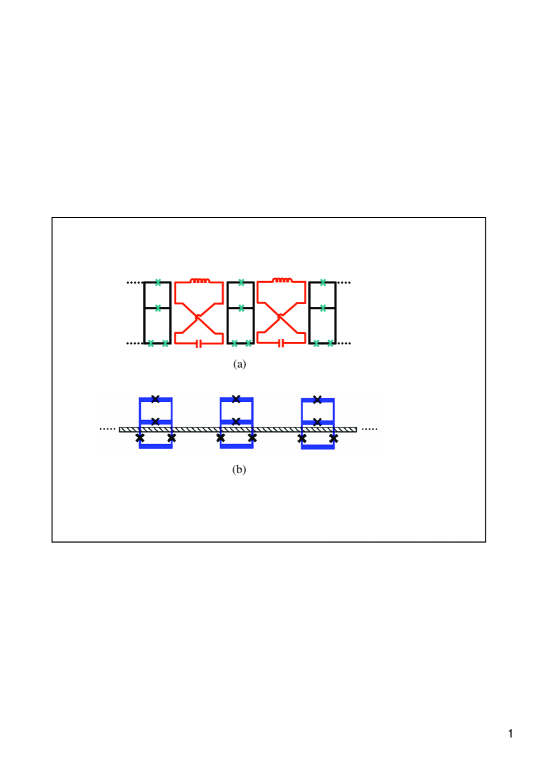
Figure 6: (Color online) Schematics to scale up the coupling system. (a) Each qubit is coupled with the nearest neighbors by twisted LC resonators. (b) All qubits are interacting with a common TLR resonator on top of the qubits array.

We illustrate two possible ways to scale up the two-qubit system. In Fig. 6 (a), a nearest-neighbor coupled qubits are sketched. They form a transverse Ising chain which can be used to implement quantum state transfer Bose (2003); Song and Sun (2005); Lyakhov and Bruder (2005) and quantum information storage Wang et al. (2005). It is possible to extend this configuration to 2D Ising model. Fig. 6 (b) shows an example to realize selective coupling between multiple qubits by a single quantum bus (such as a transmission line resonator).

For nominally same parameters, there is natural spread of the junctions critical currents. This coupling mechanism is robust to the difference of $\alpha_{0}^{\left(1\right)}$ and $\alpha_{0}^{\left(2\right)}$ because the free Hamiltonian commutes with the interaction Hamiltonian. As such, in the sample fabrication process, the requirements on homogeneity and reproducibility can be relaxed and meet with current production technology. The additional on-site control lines require only one more layer.

The qubit-resonator interaction commutes with the qubit free Hamiltonian. This feature enables quantum non-demolition (QND) measurement on superconducting qubit biased at the optimal point Blais et al. (2004). This QND measurement is realizable even in the ultra-strong coupling limit Lupascu et al. (2007).

References

- Makhlin et al. (2001) Y. Makhlin, G. Schön, and A. Shnirman, Rev. Mod. Phys. 73, 357 (2001).
- You and Nori (2005) J. Q. You and F. Nori, Phys. Today 58, 42 (2005).
- Wendin and Shumeiko (2006) G. Wendin and V. Shumeiko, in Handbook of Theoretical and Computational Nanotechnology (ASP, Los Angeles, 2006).
- Clarke and Wilhelm (2008) J. Clarke and F. K. Wilhelm, Nature 453, 1031 (2008).
- Nakamura et al. (1999) Y. Nakamura, Yu. A. Pashkin, and J. S. Tsai, Nature (London) 398, 786 (1999).
- Vion et al. (2002) D. Vion, A. Aassime, A. Cottet, P. Joyez, H. Pothier, C. Urbina, D. Esteve, and M. H. Devoret, Science 296, 886 (2002).
- Yu et al. (2002) Y. Yu, S. Han, X. Chu, S.-I. Chu, and Z. Wang, Science 296, 889 (2002).
- Martinis et al. (2002) J. M. Martinis , S. Nam, J. Aumentado, and C. Urbina, Phys. Rev. Lett. 89, 117901 (2002).
- Chiorescu et al. (2003) I. Chiorescu, Y. Nakamura, C. J. P. M. Harmans, and J. E. Mooij, Science 299, 1869 (2003).
- Saito et al. (2004) S. Saito, M. Thorwart, H. Tanaka, M. Ueda, H. Nakano, K. Semba, and H. Takayanagi, Phys. Rev. Lett. 93, 037001 (2004).
- Johansson et al. (2006) J. Johansson, S. Saito, T. Meno, H. Nakano, M. Ueda, K. Semba, and H. Takayanagi, Phys. Rev. Lett. 96, 127006 (2006).
- Deppe et al. (2008) F. Deppe, M. Mariantoni, E. P. Menzel, A. Marx, S. Saito, K. Kakuyanagi, H. Tanaka, T. Meno, K. Semba, H. Takayanagi, E. Solano,and R. Gross, Nature Physics 4, 686 (2008).
- Pashkin et al. (2003) Yu. A. Pashkin, T. Yamamoto, O. Astafiev, Y. Nakamura, D. V. Averin, and J. S. Tsai, Nature (London) 421, 823 (2003).
- Yamamoto et al. (2003) T. Yamamoto, Yu. A. Pashkin, O. Astafiev, Y. Nakamura, and J. S. Tsai, Nature (London) 425, 941 (2003).
- Berkley et al. (2003) A. J. Berkley, H. Xu, R. C. Ramos, M. A. Gubrud, F. W. Strauch, P. R. Johnson, J. R. Anderson, A. J. Dragt, C. J. Lobb, and F. C. Wellstood, Science 300, 1548 (2003).
- Johnson et al. (2003) P. R. Johnson, F. W. Strauch, A. J. Dragt, R. C. Ramos, C. J. Lobb, J. R. Anderson, and F. C. Wellstood, Phys. Rev. B. 67, 020509(R) (2003).
- Izmalkov et al. (2004) A. Izmalkov, M. Grajcar, E. Il’ichev, Th. Wagner, H.-G. Meyer, A. Yu. Smirnov, M. H. S. Amin, A. M. Maassen van den Brink, and A. M. Zagoskin, Phys. Rev. Lett. 93, 037003 (2004).
- Xu et al. (2005) H. Xu, F. W. Strauch, S. K. Dutta, P. R. Johnson, R. C. Ramos, A. J. Berkley, H. Paik, J. R. Anderson, A. J. Dragt, C. J. Lobb, et al., Phys. Rev. Lett. 94, 027003 (2005).
- McDermott et al. (2005) R. McDermott, R. W. Simmonds, M. Steffen, K. B. Cooper, K. Cicak, K. D. Osborn, S. Oh, D. P. Pappas, and J. M. Martinis, Science 307, 1299 (2005).
- Majer et al. (2005) J. B. Majer, F. G. Paauw, A. C. J. ter Haar, C. J. P. M. Harmans, and J. E. Mooij, Phys. Rev. Lett. 94, 090501 (2005).
- Plourde et al. (2005) B. L. T. Plourde, T. L. Robertson, P. A. Reichardt, T. Hime, S. Linzen, C.-E. Wu, and J. Clarke, Phys. Rev. B 72, 060506(R) (2005).
- Hime et al. (2006) T. Hime, P. A. Reichardt, B. L. T. Plourde, T. L. Robertson, C.-E. Wu, A. V. Ustinov, and J. Clarke, Science 314 , 1427 (2006).
- Harris et al. (2007) R. Harris, A. J. Berkley, M. W. Johnson, P. Bunyk, S. Govorkov, M. C. Thom, S. Uchaikin, A. B. Wilson, J. Chung, E. Holtham, et al., Phys. Rev. Lett. 98, 177001 (2007).
- Ploeg et al. (2007) S. H. W. van der Ploeg, A. Izmalkov, A. M. van den Brink, U. Hübner, M. Grajcar, E. Il’ichev, H.-G. Meyer, and A. M. Zagoskin, Phys. Rev. Lett. 98, 057004 (2007).
- Niskanen et al. (2007) A. O. Niskanen, K. Harrabi, F. Yoshihara, Y. Nakamura, S. Lloyd, and J. S. Tsai, Science 316, 723 (2007).
- Plantenberg et al. (2007) J. H. Plantenberg, P. C. de Groot, C. J. P. M. Harmans, and J. E. Mooij, Nature 447, 836 (2007).
- Sillanpää et al. (2007) M. A. Sillanpää, J. I. Park, and R. W. Simmonds, Nature (London) 449, 438 (2007).
- Majer et al. (2007) J. Majer, J. M. Chow, J. M. Gambetta, J. Koch, B. R. Johnson, J. A. Schreier, L. Frunzio, D. I. Schuster, A. A. Houck, A. Wallraff, et al., Nature (London) 449, 443 (2007).
- Makhlin et al. (1999) Y. Makhlin, G. Schön, and A. Shnirman, Nature 398, 305 (1999).
- You et al. (2002) J. Q. You, J. S. Tsai, and F. Nori, Phys. Rev. Lett. 89, 197902 (2002).
- Averin and Bruder (2003) D. V. Averin and C. Bruder, Phys. Rev. Lett. 91, 057003 (2003).
- Wang et al. (2004) Y. D. Wang, P. Zhang, D. L. Zhou, and C. P. Sun, Phys. Rev. B 70, 224515 (2004).
- Plourde et al. (2004) B. L. T. Plourde, J. Zhang, K. B. Whaley, F. K. Wilhelm, T. L. Robertson, T. Hime, S. Linzen, P. A. Reichardt, C.-E. Wu, and J. Clarke, Phys. Rev. B (R) 70, 140501(R) (2004).
- Rigetti et al. (2005) C. Rigetti, A. Blais, and M. Devoret, Phys. Rev. Lett. 94, 240502 (2005).
- Liu et al. (2006) Y.-x. Liu, L. F. Wei, J. S. Tsai, and F. Nori, Phys. Rev. Lett. 96, 067003 (2006); Y.-x. Liu, L. F. Wei, J. R. Johansson, J. S. Tsai, and F. Nori, Phys. Rev. B 76, 144518 (2007).
- Bertet et al. (2006) P. Bertet, C. J. P. M. Harmans, and J. E. Mooij, Phys. Rev. B 73, 064512 (2006).
- Niskanen et al. (2006) A. O. Niskanen, Y. Nakamura, and J. S. Tsai, Phys. Rev. B 73, 094506 (2006).
- Grajcar et al. (2006) M. Grajcar, A. Izmalkov, S. H. W. van der Ploeg, S. Linzen, T. Plecenik, Th. Wagner, U. Hübner, E. Il’ichev, H.-G. Meyer, A. Yu. Smirnov, et al., Phys. Rev. Lett. 96, 047006 (2006).
- Paraoanu (2006) G. S. Paraoanu, Phys. Rev.B 74, 140504(R) (2006).
- Ashhab et al. (2006) S. Ashhab, S. Matsuo, N. Hatakenaka, and F. Nori, Phys. Rev. B 74, 184504 (2006); S. Ashhab, et al., ibid, 77, 014510 (2008 )
- Blais et al. (2007) A. Blais, J. Gambetta, A. Wallraff, D. I. Schuster, S. M. Girvin, M. H. Devoret, and R. J. Schoelkopf, Phys. Rev. A 75, 032329 (2007).
- Nakano et al. (2007) H. Nakano, K. Kakuyanagi, M. Ueda, and K. Semba, App. Phys. Lett. 91, 032501 (2007).
- Mooij et al. (1999) J. E. Mooij, T. P. Orlando, L. Levitov, L. Tian, C. H. van der Wal, and S. Lloyd, Science 285, 1036 (1999).
- Orlando et al. (1999) T. P. Orlando, J. E. Mooij, L. Tian, C. H. van der Wal, L. S. Levitov, S. Lloyd, and J. J. Mazo, Phys. Rev. B 60, 15398 (1999).
- Wilhelm and Semba (2006) F. K. Wilhelm and K. Semba, in Physical Realization of Quantum Computing (World Scientific, Singapore, 2006).
- You et al. (2005) J. Q. You, Y. Nakamura, and F. Nori, Phys. Rev. B 71, 024532 (2005).
- Kerman (2008) A. J. Kerman, and W. D. Oliver, Phys. Rev. Lett. 101, 070501 (2008).
- Milburn (1999) G. Milburn, quant-ph/9908037 (1999).
- Sørensen and Mølmer (1999) A. Sørensen and K. Mølmer, Phys. Rev. Lett. 82, 1971 (1999).
- Sørensen and Mølmer (2000) A. Sørensen and K. Mølmer, Phys. Rev. A 62, 022311 (2000).
- Wang et al. (2001) X. Wang, A. Sørensen, and K. Mølmer, Phys. Rev. Lett. 86, 3907 (2001).
- Sackett et al. (2000) C. A. Sackett, D. Kielpinski, B. E. King, C. Langer, V. Meyer, C. J. Myatt, M. Rowe, Q. A. Turchette, W. M. Itano, D. J. Wineland, and C. Monroe, Nature 404, 256 (2000).
- Leibfried et al. (2003) D. Leibfried, B. De Marco, V. Meyer, D. Lucas, M. Barrett, J. Britton, W. M. Itano, B. Jelenković, C. Langer, T. Rosenband, and D. J. Wineland Nature 422, 412 (2003).
- Haljan et al. (2005) P. C. Haljan, P. J Lee, K.-A. Brickman, M. Acton, L. Deslauriers, and C. Monroe Phys. Rev. A 72, 062316 (2005).
- Home et al. (2006) J. P. Home, M. J McDonnell, D. M. Lucas, G. Imreh, B. C. Keitch, D. J. Szwer, N. R Thomas, S.C. Webster, D. N. Stacey, and A. M. Steane New. J. Phys. 8, 188 (2006).
- Wei and Norman (1963) J. Wei and E. Norman, J. Math. Phys. 4, 575 (1963).
- Barenco et al. (1995) A. Barenco, C. H. Bennett, R. Cleve, D. P. DiVincenzo, N. Margolus, P. Shor, T. Sleator, J. A. Smolin, and H. Weinfurter, Phys. Rev. A 52, 3457 (1995).
- Bose (2003) S. Bose, Phys. Rev. Lett. 91, 207901 (2003).
- Song and Sun (2005) Z. Song and C. P. Sun, Low Temp. Phys. 31, 686 (2005).
- Lyakhov and Bruder (2005) A. Lyakhov and C. Bruder, New J. Phys. 7, 181 (2005).
- Wang et al. (2005) Y. D. Wang, Z. D. Wang, and C. P. Sun, Phys. Rev. B 72, 172507 (2005).
- Blais et al. (2004) A. Blais, R.-S. Huang, A. Wallraff, S. M. Girvin, and R. J. Schoelkopf, Phys. Rev. A 69, 062320 (2004).
- Lupascu et al. (2007) A. Lupaşcu, S. Saito, T. Picot, P. C. de Groot, C. J. P. M. Harmans, and J. E. Mooij, Nature Physics 3, 119 (2007).