Spin squeezing in a bimodal condensate: spatial dynamics and particle losses

Abstract

We propose an analytical method to study the entangled spatial and spin dynamics of interacting bimodal Bose-Einstein condensates. We show that at particular times during the evolution spatial and spin dynamics disentangle and the spin squeezing can be predicted by a simple two-mode model. We calculate the maximum spin squeezing achievable in experimentally relevant situations with Sodium or Rubidium bimodal condensates, including the effect of the dynamics and of one, two and three-body losses.

1 Introduction

In atomic systems effective spins are collective variables that can be defined in terms of orthogonal bosonic modes. In this paper the two modes we consider are two different internal states of the atoms in a bimodal Bose-Einstein condensate. States with a large first order coherence between the two modes, that is with a large mean value of the effective spin component in the equatorial plane of the Bloch sphere, can still differ by their spin fluctuations. For an uncorrelated ensemble of atoms, the quantum noise is evenly distributed among the spin components orthogonal to the mean spin. However quantum correlations can redistribute this noise and reduce the variance of one spin quadrature with respect to the uncorrelated case, achieving spin squeezing Ueda ; manip . Spin-squeezed states are multi-particle entangled states that have practical interest in atom interferometry, and high precision spectroscopy Wineland . Quantum entanglement to improve the precision of spectroscopic measurements has already been used with trapped ions Liebfried and it could be used in atomic clocks where the standard quantum limit has already been reached Santarelli .

A promising all-atomic route to create spin squeezing in bimodal condensates, proposed in Nature , relies on the Kerr-type non linearity due to elastic interactions between atoms. Quite analogously to what happens to a coherent state in a nonlinear Kerr medium in optics coherent , an initial “phase state” or coherent spin state, where all the effective spins point at the same direction, dynamically evolves into a correlated spin-squeezed state. A straightforward way to produce the initial phase state in a bimodal condensate is to start with one atomic condensate in a given internal state $a$ and perform a $\pi/2$-pulse coupling coherently the internal state $a$ to a second internal state $b$ Cornell . However, as the strength of the interactions between two atoms $a-a$, $b-b$ and $a-b$ are in general different, the change in the mean field energy excites the spatial dynamics of the condensate wave functions. In the evolution subsequent to the pulse, the spin dynamics creating squeezing and the spatial dynamics are entangled Nature ; EPJD ; Sorensen ; Dutton and occur on the same time scale set by an effective interaction parameter $\chi$. This makes it a priori more difficult to obtain simple analytical results.

In this paper we develop a simple formalism which allows us to calculate analytically or semi analytically the effect of the spatial dynamics on spin squeezing. In Section 2 we present our dynamic model. Using our treatment we show that at particular times in the evolution the spatial dynamics and the spin dynamics disentangle and the dynamical model gives the same results as a simple two-mode model. We also identify configurations of parameters in which the simple two mode-model is a good approximation at all times. Restricting to a two-mode model, in Section 3 we generalize our analytical results of PRLlosses on optimal spin squeezing in presence of particle losses to the case of overlapping and non-symmetric condensates.

In Sections 4 and 5, we apply our treatment to cases of practical interest. We first consider a bimodal ⁸⁷Rb condensate. Rb is one of the most common atoms in BEC experiments and it is a good candidate for atomic clocks using trapped atoms on a chip clockRb . Restricting to states which are equally affected by a magnetic field to first order, the most common choices are $|F=1,m=-1\rangle$ and $|F=2,m=1\rangle$ which can be magnetically trapped, or $|F=1,m=1\rangle$ and $|F=2,m=-1\rangle$ that must be trapped optically but for which there exists a low-field Feshbach resonance which can be used to reduce the inter-species scattering length Sengstock ; Widera . Indeed a particular feature of these Rb states is that the three $s$-wave scattering lengths characterizing interactions between $a-a$, $b-b$ and $a-b$ atoms are very close to each other. A consequence is that the squeezing dynamics is very slow when the two condensates overlap. The inter-species Feshbach resonance can be used to overcome this problem and speed up the dynamics Widera .

In schemes involving the $|F=2,m=\pm 1\rangle$ of Rubidium, the main limit to the maximum squeezing achievable is set by the large two-body losses rate in these states. As a second case of experimental interest we then consider Na atoms in the $|F=1,m_{F}=\pm 1\rangle$ states Nature . Although theses states have opposite shifts in a magnetic field, they present the advantage of negligible two-body losses. Using our analytical optimization procedure, we calculate the maximum squeezing achievable in this system including the effect of spatial dynamics and particle losses.

In Section 5 we examine a different scenario for Rb condensates in which, instead of changing the scattering length, one would spatially separate the two condensates after the mixing $\pi/2$ pulse and hold them separately during a well chosen squeezing time. An interesting feature of this scheme is that the squeezing dynamics acts only when the clouds are spatially separated and it freezes out when the two clouds are put back together so that one could prepare a spin squeezed state and then keep it for a certain time PRLlosses . State-selective potentials for ⁸⁷Rb in $|F=1,m=-1\rangle$ and $|F=2,m=1\rangle$ clockRb have recently been implemented on an atom chip, and such scheme could be of experimental interest.

2 Dynamical spin squeezing model

In this section we develop and compare dynamical models for spin squeezing. No losses will be taken into account in this section.

2.1 State evolution

We consider the model Hamiltonian

$$H = \int d^{3}\vec{r}\>\sum_{\varepsilon=a,b}\left[\hat{\psi}^{\dagger}_{\varepsilon}h_{\varepsilon}\hat{\psi}_{\varepsilon}+\frac{1}{2}g_{\varepsilon\varepsilon}\hat{\psi}^{\dagger}_{\varepsilon}\hat{\psi}^{\dagger}_{\varepsilon}\hat{\psi}_{\varepsilon}\hat{\psi}_{\varepsilon}\right]$$ (1)

$$+ g_{ab}\hat{\psi}^{\dagger}_{b}\hat{\psi}^{\dagger}_{a}\hat{\psi}_{a}\hat{\psi}_{b}\,$$

where $h_{\varepsilon}$ is the one-body hamiltonian including kinetic energy and external trapping potential

$$h_{\varepsilon}=-\frac{\hbar^{2}\Delta}{2m}+U^{\mbox{ \small ext}}_{\varepsilon}(\vec{r}\,)\,.$$ (2)

The interactions constants $g_{\varepsilon\varepsilon^{\prime}}$ are related to the corresponding $s$-wave scattering lengths $g_{\varepsilon\varepsilon^{\prime}}=4\pi\hbar^{2}a_{\varepsilon\varepsilon^{\prime}}/M$ characterizing a cold collision between an atom in state $\varepsilon$ with an atom in state $\varepsilon^{\prime}$ ($\varepsilon,\varepsilon^{\prime}=a,b$), and $M$ is the mass of one atom.

We assume that we start from a condensate with $N$ atoms in the internal state $a$; the stationary wave function of the condensate is $\phi_{0}(\vec{r}\,)$. After a $\pi/2$ pulse, a phase state is created, which is our initial state:

$$|\Psi(0)\rangle=\frac{1}{\sqrt{N!}}\left[C_{a}a^{\dagger}_{|\phi_{0}\rangle}+C_{b}b^{\dagger}_{|\phi_{0}\rangle}\right]^{N}|0\rangle$$ (3)

where $C_{a}$, $C_{b}$ are mixing coefficients with $|C_{a}|^{2}+|C_{b}|^{2}=1$ and the operator $a^{\dagger}_{|\phi_{0}\rangle}$ creates a particle in the internal state $a$ with wave function $\phi_{0}$. To describe the entangled evolution of the spin dynamics and the external dynamics of the wave functions, it is convenient to introduce Fock states with well defined number of particles in $|a\rangle$ and $|b\rangle$, these numbers being preserved during time evolution subsequent to the mixing pulse. Expanded over the Fock states, the initial state (3) reads:

$$|\Psi(0)\rangle=\sum^{N}_{N_{a}=0}\left(\frac{N!}{N_{a}!N_{b}!}\right)^{1/2}C_{a}^{N_{a}}C_{b}^{N_{b}}|N_{a}:\phi_{0},N_{b}:\phi_{0}\rangle,$$ (4)

where $N_{b}=N-N_{a}$, and

$$|N_{a}:\phi_{a},N_{b}:\phi_{b}\rangle=\frac{\left[{a}^{\dagger}_{|\phi_{a}(N_{a},N_{b})\rangle}\right]^{N_{a}}}{\sqrt{N_{a}!}}\frac{\left[{b}^{\dagger}_{|\phi_{b}(N_{a},N_{b})\rangle}\right]^{N_{b}}}{\sqrt{N_{b}!}}|0\rangle\,.$$ (5)

Within an Hartee-Fock type ansatz for the $N$-body state vector, we calculate the evolution of each Fock state in (4). We get EPJD :

$$|N_{a}:\phi_{0},N_{b}:\phi_{0}\rangle\rightarrow e^{-iA(N_{a},N_{b};\,t)/\hbar}$$

$$\hskip 28.45274pt\times|N_{a}:\phi_{a}(N_{a},N_{b};t),N_{b}:\phi_{b}(N_{a},N_{b};t)\rangle\,,$$ (6)

where $\phi_{a}(N_{a},N_{b};t)$ and $\phi_{b}(N_{a},N_{b};t)$ are solutions of the coupled Gross-Pitaevskii equations:

$$i\hbar\partial_{t}\phi_{\varepsilon}=\left[h_{\varepsilon}+(N_{\varepsilon}-1)g_{\varepsilon\varepsilon}|\phi_{\varepsilon}|^{2}+N_{\varepsilon}^{\prime}g_{\varepsilon\varepsilon^{\prime}}|\phi_{\varepsilon^{\prime}}|^{2}\right]\phi_{\varepsilon}$$ (7)

here with the initial conditions

$$\phi_{a}(0)=\phi_{b}(0)=\phi_{0}\,,$$ (8)

and the time dependent phase factor $A$ solves:

$$\frac{d}{dt}A(N_{a},N_{b};t) = -\sum_{\varepsilon=a,b}N_{\varepsilon}(N_{\varepsilon}-1)\frac{g_{\varepsilon\varepsilon}}{2}\int d^{3}r|\phi_{\varepsilon}|^{4}$$ (9)

$$- N_{a}N_{b}g_{ab}\int d^{3}r|\phi_{a}|^{2}|\phi_{b}|^{2}\,.$$

With this treatment we fully include the quantum dynamics of the two condensate modes $a$ and $b$, as one does for the simple two modes model, but also including the spatial dynamics of the two modes and their dependence on the number of particles. The approximation we make is to neglect all the other modes orthogonal to the condensates which would be populated thermally. An alternative method is to use a number conserving Bogoliubov theory that explicitly includes the operators of the condensates as in Sorensen . In that case all the modes are present but the modes orthogonal to the condensates are treated in a linearized way. In Sorensen , the author compares the number conserving Bogoliubov approach to our approach using many Gross-Piaevskii equations, also used in Nature , and he finds very similar result for the spin squeezing. He also finds that within the Bogoliuobov approximation the thermally excited modes strictly do not affect the squeezing in the scheme we consider here. If the number conserving Bogoliubov has the advantage of being systematic, our approach, supplemented with a further approximation (the modulus-phase approximation introduced in Sect. 2.3) allows us to get some insight and obtain simple analytical results.

2.2 Calculation of spin squeezing

The effective collective spin of a two-components BEC can be represented on the Bloch sphere as shown in Fig.1(Top). Formally, we introduce three spin operators in terms of field operators Nature

$$S_{x}= \dfrac{1}{2}\int d^{3}r[\hat{\psi}^{\dagger}_{b}(\vec{r}\,)\hat{\psi}_{a}(\vec{r}\,)+\hat{\psi}^{\dagger}_{a}(\vec{r}\,)\hat{\psi}_{b}(\vec{r}\,)],$$ (10)

$$S_{y}= \dfrac{i}{2}\int d^{3}r[\hat{\psi}^{\dagger}_{b}(\vec{r}\,)\hat{\psi}_{a}(\vec{r}\,)-\hat{\psi}^{\dagger}_{a}(\vec{r}\,)\hat{\psi}_{b}(\vec{r}\,)],$$ (11)

$$S_{z}= \dfrac{1}{2}\int d^{3}r[\hat{\psi}^{\dagger}_{a}(\vec{r}\,)\hat{\psi}_{a}(\vec{r}\,)-\hat{\psi}^{\dagger}_{b}(\vec{r})\hat{\psi}_{b}(\vec{r})].$$ (12)

Definitions (10)-(12) explicitly take into account the spatial wave functions of the condensate and depend in particular on the overlap between the two modes.

Referring to the Fig.1(Top) we introduce the polar angles $\vartheta$ and $\varphi$ giving the direction $z^{\prime}$ of the mean spin; $\vartheta$ determines the relative mean atom number in the two internal states, $\cos\vartheta=|C_{a}|^{2}-|C_{b}|^{2}$, while the azimuthal angle $\varphi$ corresponds to the relative phase between the components, $\varphi=\arg(C_{a}^{\ast}C_{b})$.

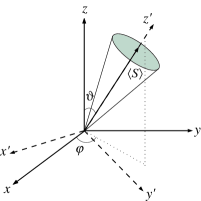
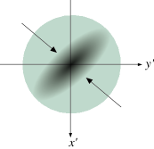
Figure 1: (Top) average spin. (Bottom) variance of the the spin components in the plane orthogonal to the mean spin.

The minimal variance of the spin in the plane $(x^{\prime},y^{\prime})$ orthogonal to the mean spin $\Delta S_{\perp,\mbox{\small min}}^{2}$, represented in Fig. 1(Bottom), is given by

$$\Delta S_{\perp,\mbox{\small min}}^{2}=\frac{1}{2}(\Delta S_{x^{\prime}}^{2}+\Delta S_{y^{\prime}}^{2}-|\Delta S_{-}^{2}|)$$ (13)

where we introduced

$$S_{-}=S_{x^{\prime}}-iS_{y^{\prime}}\,.$$ (14)

The degree of squeezing is then quantified by the parameter Nature ; Wineland

$$\xi^{2}=\frac{N\Delta S_{\perp,\mbox{\small min}}^{2}}{\langle S\rangle^{2}},$$ (15)

where $\langle S\rangle$ is the length of the average spin.

When expressed in the original frame of reference, the minimal variance in the orthogonal plane is:

$$\Delta S_{\perp,\mbox{\small min}}^{2} = \frac{1}{2}(\cos^{2}\vartheta\cos^{2}\varphi+\sin^{2}\varphi)\Delta S_{x}^{2}$$ (16)

$$+ \frac{1}{2}(\cos^{2}\vartheta\sin^{2}\varphi+\cos^{2}\varphi)\Delta S_{y}^{2}$$

$$+ \frac{1}{2}\sin^{2}\vartheta\Delta S_{z}^{2}-\frac{1}{4}\sin^{2}\vartheta\sin 2\varphi\Delta_{xy}$$

$$- \frac{1}{4}\sin 2\vartheta\cos\varphi\Delta_{zx}-\frac{1}{4}\sin 2\vartheta\sin\varphi\Delta_{yz}$$

$$- \frac{1}{2}\sqrt{\tilde{A}^{2}+\tilde{B}^{2}}$$

where

$$\tilde{A} = (\sin^{2}\varphi-\cos^{2}\vartheta\cos^{2}\varphi)\Delta S_{x}^{2}\phantom{\frac{1}{2}}$$ (17)

$$+ (\cos^{2}\varphi-\cos^{2}\vartheta\sin^{2}\varphi)\Delta S_{y}^{2}-\sin^{2}\vartheta\Delta S_{z}^{2}$$

$$- \frac{1}{2}(1+\cos^{2}\vartheta)\sin 2\varphi\Delta_{xy}+\frac{1}{2}\sin 2\vartheta\cos\varphi\Delta_{zx}$$

$$+ \frac{1}{2}\sin 2\vartheta\sin\varphi\Delta_{yz}\>;$$

$$\tilde{B} = \cos\vartheta\sin 2\varphi(\Delta S_{x}^{2}-\Delta S_{y}^{2})-\cos\vartheta\cos 2\varphi\Delta_{xy}$$ (18)

$$- \sin\vartheta\sin\varphi\Delta_{zx}+\sin\vartheta\cos\varphi\Delta_{yz}\>;$$

and where we introduced the correlations

$$\Delta_{ij}=\langle S_{i}S_{j}+S_{j}S_{i}\rangle-2\langle S_{i}\rangle\langle S_{j}\rangle,\hskip 14.22636pti\neq j=x,y,z\,.$$ (19)

The spin squeezing is then calculated in terms of averages of field operators products, with the state of the system at time $t$, obtained by evolving equation (4) with equation (6). To calculate the averages one needs to compute the action of the field operators $\hat{\psi}_{a}$ $\hat{\psi}_{b}$ on the Fock states (5) notecalc1 ,

$$\hat{\psi}_{a}(\vec{r}) |N_{a}:\phi_{a}(N_{a},N_{b}),N_{b}:\phi_{b}(N_{a},N_{b})\rangle$$

$$= \phi_{a}(N_{a},N_{b},\vec{r})\sqrt{N_{a}}$$

$$\times |N_{a}-1:\phi_{a}(N_{a},N_{b}),N_{b}:\phi_{b}(N_{a},N_{b})\rangle,$$

$$\hat{\psi}_{b}(\vec{r}) |N_{a}:\phi_{a}(N_{a},N_{b}),N_{b}:\phi_{b}(N_{a},N_{b})\rangle$$

$$= \phi_{b}(N_{a},N_{b},\vec{r})\sqrt{N_{b}}$$

$$\times |N_{a}:\phi_{a}(N_{a},N_{b}),N_{b}-1:\phi_{b}(N_{a},N_{b})\rangle.$$ (21)

The explicit expressions of the averages needed to calculate the spin squeezing parameter are given in Appendix A. These quantum averages correspond to an initial state with a well-defined number of particles $N$. In case of fluctuations in the total number of particles where the density matrix of the system is a statistical mixture of states with a different number of particles, a further averaging of $N$ over a probability distribution $P(N)$ is needed EPJD ; EPJDLoss .

2.3 Dynamical modulus-phase approach

In principle, equations (7)-(9) can be solved numerically for each Fock state in the sum equation (4), and the squeezing can be computed as explained in the previous section. However, for a large number of atoms and especially in three dimensions and in the absence of particular symmetries (e.g. spherical symmetry) this can be a very heavy numerical task. To overcome this difficulty, in order to develop an analytical approach, we can exploit the fact that for large $N$ in the initial state (4) the distributions of the number of atoms $N_{a}$ and $N_{b}$ are very peaked around their average values with a typical width of order $\sqrt{N}$. Moreover, assuming that possible fluctuations in the total number of particles are described by a distribution $P(N)$ having a width much smaller than the average of the total number of particles $\bar{N}$, we can limit to $N_{a}$ and $N_{b}$ close to $\bar{N}_{a}=|C_{a}|^{2}\bar{N}$ and $\bar{N}_{b}=|C_{b}|^{2}\bar{N}$. We then split the condensate wave function into modulus and phase

$$\phi_{\varepsilon}=|\phi_{\varepsilon}|\exp(i\theta_{\varepsilon})\;\hskip 14.22636pt\varepsilon=a,b\,,$$ (22)

and we assume that the variation of the modulus over the distribution of $N_{\varepsilon}$ can be neglected while we approximate the variation of the phase by a linear expansion around $\bar{N}_{\varepsilon}$ EPJD . The approximate condensate wave functions read

$$\phi_{\varepsilon}(N_{a},N_{b})\simeq\bar{\phi}_{\varepsilon}\exp\left[i\sum_{\varepsilon^{\prime}=a,b}(N_{\varepsilon^{\prime}}-\bar{N}_{\varepsilon^{\prime}})(\partial_{N_{\varepsilon^{\prime}}}\theta_{\varepsilon})_{\bar{N}_{a},\bar{N}_{b}}\right]$$ (23)

where $\bar{\phi}_{\varepsilon}\equiv\phi_{\varepsilon}(N_{a}=\bar{N}_{a},N_{b}=\bar{N}_{b})$.

The modulus phase approximation takes into account, in an approximate way, the dependence of the condensate wave functions on the number of particles. It is precisely this effect that is responsible of entanglement between spatial dynamics and spin dynamics.

As explained in Appendix B, all the relevant averages needed to calculate spin squeezing can then be expressed in terms of $\bar{\phi}_{\varepsilon}$ and of three time and position dependent quantities:

$$\chi_{d}(\vec{r})=\frac{1}{2}\left[(\partial_{N_{a}}-\partial_{N_{b}})(\theta_{a}-\theta_{b})\right]_{\bar{N}_{a},\bar{N}_{b}},$$ (24)

$$\chi_{s}(\vec{r})=\frac{1}{2}\left[(\partial_{N_{a}}+\partial_{N_{b}})(\theta_{a}-\theta_{b})\right]_{\bar{N}_{a},\bar{N}_{b}},$$ (25)

$$\chi_{0}(\vec{r})=\frac{1}{2}\left[(\partial_{N_{a}}-\partial_{N_{b}})(\theta_{a}+\theta_{b})\right]_{\bar{N}_{a},\bar{N}_{b}}\,.$$ (26)

In some cases (see Sect. 2.4) these quantities can be explicitly calculated analytically. To calculate the squeezing in the general case, it is sufficient to evolve a few coupled Gross-Pitaevskii equations (7) for different values of $N_{a}$, $N_{b}$, to calculate numerically the derivatives of the phases appearing in (24)-(26). Although we do not expect a perfect quantitative agreement with the full numerical model for all values of parameters, we will see that the analytical model catches the main features and allows us to interpret simply the results.

In the particular case of stationary wave functions of the condensates, the parameters $\chi_{d}$, $\chi_{s}$ and $\chi_{0}$ become space-independent:

$$\chi_{d}^{\text{st}} = -\frac{\left[(\partial_{N_{a}}-\partial_{N_{b}})({\mu}_{a}-{\mu}_{b})\right]_{\bar{N}_{a},\bar{N}_{b}}}{2\hbar}\,t$$ (27)

$$\chi_{s}^{\text{st}} = -\frac{\left[(\partial_{N_{a}}+\partial_{N_{b}})({\mu}_{a}-{\mu}_{b})\right]_{\bar{N}_{a},\bar{N}_{b}}}{2\hbar}\,t$$ (28)

$$\chi_{0}^{\text{st}} = \chi_{s}^{\text{st}}\,.$$ (29)

In this case we recover a simple two-mode model. Equations (27)-(28) will be used in section 3. In that contest we will rename $\chi_{d}^{\text{st}}/t=-\chi$ and $\chi_{s}^{\text{st}}/t=-\tilde{\chi}$ to shorten the notations.

To test our modulus-phase dynamical model, in Fig. 2, we consider a situation in which the external dynamics is significantly excited after the $\pi/2$ pulse which populates the state $b$. Parameters correspond to a bimodal Rb condensate in $|F=1,m_{F}=1\rangle$ and $|F=2,m_{F}=-1\rangle$ with $\bar{N}_{a}=\bar{N}_{b}=5\times 10^{4}$ and where a Feshbach resonance is used to reduce $a_{ab}$ by about 10% with respect to its bare value Sengstock ; Widera . The considered harmonic trap is very steep $\omega=2\pi\times 2$ kHz. In the figure we compare our modulus-phase approach (dashed line) with the full numerical solution (solid line) and with a stationary calculation using (27)-(28) (dash-dotted line) which is equivalent to a two-mode model. The oscillation of the squeezing parameter in the two dynamical calculations (dashed line and solid line) are due to the fact that the sudden change in the mean-field causes oscillations in the wave functions whose amplitude and the frequency are different for each Fock state. From the figure, we find that our modulus-phase approach obtained integrating 5 Gross-Pitaevskii equations (dashed line) reproduces the main characteristics of the full numerical simulation using 3000 Fock states (solid line). The stationary two mode model on the other hand is not a good approximation in this case. Only for some particular times the three curves almost touch. At these times the wave functions of all the Fock states almost overlap and, as we will show in our analytical treatment, spatial dynamics and spin dynamics disentangle.

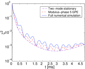
Figure 2: Spin squeezing as a function of time. Comparison of the modulus-phase model (red dashed line) with a full numerical calculation with 3000 Fock states (blue solid line) and with a stationary two-mode model (violet dash-dotted line). Spatial dynamics is strongly excited after the $\pi/2$-pulse populating a second internal state. $\omega=2\pi\times 2$ kHz, $\bar{N}_{a}=\bar{N}_{b}=5\times 10^{4}$, $m$=87 a.m.u., $a_{aa}=100.44\,r_{B}$, $a_{bb}=95.47\,r_{B}$, $a_{ab}=88.28\,r_{B}$. No particle losses. $r_{B}$ is the Bohr radius.

In Fig.3 we move to a shallow trap and less atoms.

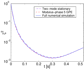
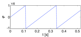
Figure 3: (Top) spin squeezing as a function of time in a case in which the spatial dynamics is weakly excited. Blue solid line: full numerical calculation with 1000 Fock states. Red dashed line: modulus-phase model. Violet dash-dotted line: stationary two-mode model. (Bottom) angle giving the direction of the mean spin projection in the equatorial plane of the Bloch sphere. Parameters: $\omega=2\pi\times 42.6$ Hz, $\bar{N}_{a}=\bar{N}_{b}=1\times 10^{4}$, $m$=87 a.m.u., $a_{aa}=100.44\,r_{B}$, $a_{bb}=95.47\,r_{B}$, $a_{ab}=88.28\,r_{B}$. No particle losses. $r_{B}$ is the Bohr radius.

We note that in this case both the modulus-phase curve and the numerical simulation are very close to the stationary two-mode model which is then a good approximation at all times.

2.4 Squeezing in the breathe-together solution

In this section we restrict to a spherically symmetric harmonic potential $U^{\mbox{\small ext}}=m\omega^{2}r^{2}/2$ identical for the two internal sates. For values of the inter particle scattering lengths such that

$$a_{ab}<a_{aa},a_{bb}$$ (30)

and for a particular choice of the mixing angle such that the mean field seen by the two condensates with $\bar{N}_{a}$ and $\bar{N}_{b}$ particles is the same:

$$\bar{N}_{a}g_{aa}+\bar{N}_{b}g_{ab}=\bar{N}_{b}g_{bb}+\bar{N}_{a}g_{ab}\equiv\bar{N}g\,,$$ (31)

the wave functions $\bar{\phi}_{a}$ and $\bar{\phi}_{b}$ solve the same Gross-Pitaevskii equation. In the Thomas-Fermi limit, the wave functions $\bar{\phi}_{a}$ and $\bar{\phi}_{b}$ share the same scaling solution $\bar{\phi}$ Scaling1 ; Scaling2 and “breathe-together” EPJD .

$$\bar{\phi}_{a}=\bar{\phi}_{b}=\bar{\phi}(\vec{r},t)\equiv\frac{e^{-i\eta(t)}}{{\cal L}^{3/2}(t)}e^{imr^{2}\dot{\cal L}(t)/2\hbar{\cal L}(t)}\bar{\phi}_{0}(\vec{r}/{\cal L}(t)\,)$$ (32)

with

$$\dot{\eta} = \frac{g}{g_{aa}}\frac{\bar{\mu}}{{\cal L}^{3}\hbar}$$ (33)

$$\frac{d^{2}{\cal L}}{dt^{2}} = \frac{g}{g_{aa}}\frac{\omega^{2}}{{\cal L}^{4}}-\omega^{2}{\cal L}\>;$$ (34)

$$\bar{\phi}_{0}(\vec{r}\,) = \left(\frac{15}{8\pi R_{0}^{3}}\right)^{1/2}\left[1-\frac{r^{2}}{R_{0}^{2}}\right]^{1/2}$$ (35)

$\bar{\mu}$ is the chemical potential of the stationary condensate before the $\pi/2$ pulse, when all the $N$ atoms are in state $a$, and $R_{0}=\sqrt{2\bar{\mu}/m\omega^{2}}$ is the corresponding Thomas-Fermi radius. The initial conditions for (34) are ${\cal L}(0)=1$ and $\dot{\cal L}(0)=0$.

Note that the scaling solution identical for the two modes $a$ and $b$ is valid only for $N_{a}=\bar{N}_{a}$, $N_{b}=\bar{N}_{b}$ and does not apply to all the wave functions $\phi_{a}(N_{a},N_{b})$ and $\phi_{b}(N_{a},N_{b})$ in the expansion equation (4). Nevertheless, an advantage of choosing the mixing angle in order to satisfy the breathe-together condition equation (31), is that the mean spin has no drift velocity. In Fig.4 we calculate the spin squeezing (Top) and the angle $\varphi$ giving the direction of the mean spin projection on the equatorial plane of the Bloch sphere (Bottom), for the same parameters as in Fig.3 except for the mixing angle that we now choose satisfying equation (31) while in Fig.3 we had $\bar{N}_{a}=\bar{N}_{b}$. Note that $\varphi$ practically does not evolve. The maximum amount of squeezing is lower in the breathe-together configuration than in the even-mixing case (see also Dutton ). However, as we will see in the next section, this conclusion does not hold when particle losses are taken into account.

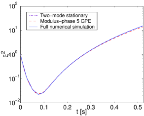
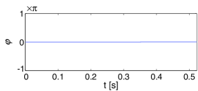
Figure 4: (Top) spin squeezing in breathe-together conditions as a function of time. Blue solid line: full numerical calculation. Red dashed line: modulus-phase model. Violet dash-dotted line: stationary two-mode model. (Bottom) angle giving the direction of the mean spin projection on the equatorial plane of the Bloch sphere. Parameters: $\omega=2\pi\times 42.6$ Hz, $\bar{N}_{a}=7432$, $\bar{N}_{b}=12568$, $m$=87 a.m.u., $a_{aa}=100.44\,r_{B}$, $a_{bb}=95.47\,r_{B}$, $a_{ab}=88.28\,r_{B}$. No particle losses. $r_{B}$ is the Bohr radius.

By linearization of $\phi_{a}(N_{a},N_{b})$ and $\phi_{b}(N_{a},N_{b})$ around the breathe-together solution $\bar{\phi}$ and using classical hydrodynamics, it is even possible to calculate analytically the parameters $\chi_{d}$ and $\chi_{s}$ relevant for the squeezing dynamics EPJD . One obtains:

$$\chi_{d}(\vec{r},t) = -\frac{1}{2\hbar}\left(\frac{2}{5}\frac{\bar{\mu}}{N}\right)\frac{g_{aa}+g_{bb}-2g_{ab}}{g_{aa}}$$ (36)

$$\times\left\{\int_{0}^{t}\frac{dt^{\prime}}{{\cal L}^{3}(t^{\prime})}+\frac{5}{2}\frac{\mbox{Im}{\cal B}(t)}{\Omega_{5}}\left[\left(\frac{r}{{\cal L}(t)R_{0}}\right)^{2}-\frac{3}{5}\right]\right\}$$

$$\chi_{s}(\vec{r},t) = \left(|C_{b}|^{2}-|C_{a}|^{2}\right)\chi_{d}=\chi_{0}(\vec{r},t)\,.$$ (37)

with

$$\Omega_{5}=\left(\frac{\bar{N}_{a}\bar{N}_{b}}{N^{2}}\frac{g_{aa}+g_{bb}-2g_{ab}}{g_{aa}}\right)^{1/2}5^{1/2}\omega$$ (38)

and where $\mbox{Im}{\cal B}(t)$ is solution of the differential equations

$$i\dot{{\cal{A}}} = \frac{\Omega_{5}}{{\cal L}^{2}(t)}{\cal{B}}$$ (39)

$$i\dot{{\cal{B}}} = \frac{\Omega_{5}}{{\cal L}^{3}(t)}{\cal{A}}$$ (40)

to be solved together with equation (34), with initial conditions ${\cal A}(0)={\cal B}(0)=1$. In practice, when we expand the condensate wave functions around the breathe-together solution equation (32) as in EPJD , we encounter the hydrodynamics operator $S$ Stringari

$$S[\alpha]\equiv-\frac{Ng_{aa}}{M}\mbox{div}[\bar{\phi}_{0}^{2}\>{\mbox{\bf grad}}\,\alpha]\,.$$ (41)

The deviation of the relative phase and the relative density from the breathe-together solution expand over two eigenmodes of $S$: A zero-energy mode which grows linearly in time and gives the dominant features of phase dynamics and squeezing (integral term in the curly brackets in Eq.(36)), and a breathing mode of frequency $\Omega_{5}$ which is responsible for the oscillations of the squeezing parameter. The fact that in breathe-together conditions and within the modulus-phase approximation $\chi_{s}=\chi_{0}$ is shown in Appendix C.

We give an example corresponding to strongly oscillating wave functions in Fig.5 where we compare the spin squeezing from the analytical theory with a numerical simulation. In the analytical formula, the entanglement between spatial degrees of freedom and spin dynamics is apparent as $\chi_{d}$ equation (36) is position dependent. The points in which the dynamical curve (dotted line) touches the stationary two mode curve (dash-dotted line) correspond to Im${\cal B}=0$ (see the bottom curve) where space and spin dynamics are disentangled. We note however that the validity conditions of classical hydrodynamics are more stringent for a mixture of condensates with rather close scattering lengths than for a single condensate EPJD . We checked numerically that in order for equation (36) to correctly predict the frequency of the oscillations in the squeezing parameter, we have to enter deeply in the Thomas-Fermi regime.

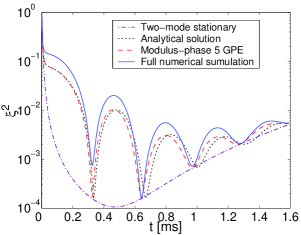
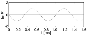
Figure 5: (Top) test of the analytical formula equation (36) in the deep Thomas-Fermi regime. Spin squeezing as a function of time. Blue solid line: full numerical calculation. Red dashed line: modulus-phase model. Black dotted line: analytical curve using equation (36). Violet dash-dotted line: stationary two-mode model using (27)-(28). (Bottom) function Im${\cal B}(t)$. Spatial and spin dynamics disentangle when Im${\cal B}(t)=0$. Parameters: $\bar{N}_{a}=\bar{N}_{b}=5\times 10^{5}$, $\omega=2\pi\times 2$ kHz, $m$=87 a.m.u., $a_{aa}=a_{bb}=0.3\,a_{ho}$, $a_{ab}=0.24\,a_{ho}$. $a_{ho}$ is the harmonic oscillator length: $a_{ho}=\sqrt{\hbar/M\omega}$. No particle losses.

2.5 “Extracted” spin squeezing

As we pointed out, the definitions equations (10)-(12) explicitly include the spatial overlap between the two modes. Here we give an alternative definition that can be used always, whether or not the modes overlap. To this aim, we introduce the time-dependent operators

$$\tilde{a} = \int d^{3}r\>\bar{\phi}^{\ast}_{a}(\vec{r},t)\hat{\psi}_{a}(\vec{r}),\;$$ (42)

$$\tilde{b} = \int d^{3}r\>\bar{\phi}^{\ast}_{b}(\vec{r},t)\hat{\psi}_{b}(\vec{r}),\;$$ (43)

where $\bar{\phi}_{\varepsilon}(\vec{r},t)$ is the solution of Gross-Pitaevskii equation (7) for mode $\varepsilon$ with $\bar{N}_{a}$, $\bar{N}_{b}$ particles. We then introduce the spin operators:

$$\tilde{S}_{x}= \dfrac{1}{2}(\tilde{b}^{\dagger}\tilde{a}+\tilde{a}^{\dagger}\tilde{b}),$$ (44)

$$\tilde{S}_{y}= \dfrac{i}{2}(\tilde{b}^{\dagger}\tilde{a}-\tilde{a}^{\dagger}\tilde{b}),$$ (45)

$$\tilde{S}_{z}= \dfrac{1}{2}(\tilde{a}^{\dagger}\tilde{a}-\tilde{b}^{\dagger}\tilde{b}).$$ (46)

In the new definition of spin squeezing calculated by the spin operators defined in equations (44)-(46), which we call the “extracted” spin squeezing, we still take into account entanglement between external motion and spin dynamics, but we give up the information about the overlap between the two modes. In Appendix D, we give the quantum averages useful to calculate the extracted spin squeezing within the modulus-phase approach described in Section 2.3. We will use this extracted spin squeezing in Section 5.

Comparing the expressions given in Appendix D with those of Appendix F (in the absence of losses), one realizes that in the stationary case, where $\chi_{d}$, $\chi_{s}$ and $\chi_{0}$ are space independent, the extracted spin squeezing dynamical model reduces to a two-mode model that we study in detail in the next section.

3 Two-mode model with Particle losses

In this section we generalize our results of PRLlosses to possibly overlapping and non-symmetric condensates. In subsection 3.1 we address the general case, while in subsection 3.2 we restrict to symmetric condensates and perform analytically an optimization of the squeezing with respect to the trap frequency and number of atoms. In the whole section, as in PRLlosses , we will limit to a two-mode stationary model and we do not address dynamical issues.

3.1 Spin squeezing in presence of losses

We consider a two-component Bose-Einstein condensate initially prepared in a phase state, that is with well defined relative phase between the two components,

$$|\Psi(0)\rangle=|\varphi\rangle\equiv\frac{\left(|C_{a}|e^{-i\varphi/2}a^{\dagger}+|C_{b}|e^{i\varphi/2}b^{\dagger}\right)^{N}}{\sqrt{N!}}|0\rangle\,.$$ (47)

When expanded over Fock states, the state (47) shows binomial coefficients which, for large $N$, are peaked around the average number of particles in $a$ and $b$, $\bar{N}_{a}$ and $\bar{N}_{b}$. In the same spirit as the “modulus-phase” approximation of subsection 2.3, we can use this fact to expand the Hamiltonian of the system to the second order around $\bar{N}_{a}$ and $\bar{N}_{b}$

$$H_{0} \simeq E(\bar{N}_{a},\bar{N}_{b})+\sum_{\varepsilon=a,b}\mu_{\varepsilon}(\hat{N}_{\varepsilon}-\bar{N}_{\varepsilon})+\frac{1}{2}\partial_{N_{\varepsilon}}\mu_{\varepsilon}(\hat{N}_{\varepsilon}-\bar{N}_{\varepsilon})^{2}$$ (48)

$$+ \frac{1}{2}\left(\partial_{N_{b}}\mu_{a}+\partial_{N_{a}}\mu_{b}\right)(\hat{N}_{a}-\bar{N}_{a})(\hat{N}_{b}-\bar{N}_{b})$$

where the chemical potentials $\mu_{\varepsilon}$ and all the derivatives of $\mu_{\varepsilon}$ should be evaluated in $\bar{N}_{a}$ and $\bar{N}_{b}$. We can write

$$H_{0}=f_{\hat{N}}+\hbar v_{\hat{N}}(\hat{N}_{a}-\hat{N}_{b})+\frac{\hbar\chi}{4}(\hat{N}_{a}-\hat{N}_{b})^{2}$$ (49)

with

$$v_{\hat{N}} = \frac{1}{2\hbar}\left[(\mu_{a}-\mu_{b})-\hbar\chi(\bar{N}_{a}-\bar{N}_{b})+\hbar\tilde{\chi}(\hat{N}-\bar{N})\right]$$ (50)

$$\chi = \frac{1}{2\hbar}\left(\partial_{N_{a}}\mu_{a}+\partial_{N_{b}}\mu_{b}-\partial_{N_{b}}\mu_{a}-\partial_{N_{a}}\mu_{b}\right)_{\bar{N}_{a},\bar{N}_{b}}\,$$ (51)

$$\tilde{\chi} = \frac{1}{2\hbar}(\partial_{N_{a}}\mu_{a}-\partial_{N_{b}}\mu_{b})_{\bar{N}_{a},\bar{N}_{b}}\,.$$ (52)

The function $f$ of the total number of particles, $\hat{N}=\hat{N}_{a}+\hat{N}_{b}$, commutes with the density operator of the system and can be omitted. The second term in equation (49) proportional to $S_{z}$ describes a rotation of the average spin vector around the $z$ axis with velocity $v_{\hat{N}}$. The third term proportional to $S_{z}^{2}$ provides the nonlinearity responsible for spin squeezing. It also provides a second contribution to the drift of the relative phase between the two condensates in the case $\bar{N}_{a}\neq\bar{N}_{b}$.

In presence of losses, the evolution is ruled by a master equation for the density operator $\rho$ of the system. In the interaction picture with respect to $H_{0}$, with one, two, and three-body losses, we have:

$$\frac{d\tilde{\rho}}{dt} = \sum_{m=1}^{3}\sum_{\varepsilon=a,b}\gamma_{\varepsilon}^{(m)}\left[{c}^{m}_{\varepsilon}\tilde{\rho}{c}^{{\dagger}m}_{\varepsilon}-\frac{1}{2}\{{c}^{{\dagger}m}_{\varepsilon}{c}^{m}_{\varepsilon},\tilde{\rho}\}\right]$$ (53)

$$+ \gamma_{ab}\left[c_{a}c_{b}\tilde{\rho}c_{a}^{\dagger}c_{b}^{\dagger}-\frac{1}{2}\{c_{a}^{\dagger}c_{b}^{\dagger}c_{a}c_{b},\tilde{\rho}\}\right]$$

where $\tilde{\rho}=e^{iH_{0}t/\hbar}\rho e^{-iH_{0}t/\hbar}$, ${c}_{a}=e^{iH_{0}t/\hbar}ae^{-iH_{0}t/\hbar}$, and similarly for $b$,

$$\gamma_{\varepsilon}^{(m)} = \frac{K_{m}^{(\varepsilon)}}{m}\int d^{3}r|\bar{\phi}_{\varepsilon}(r)|^{2m}\,,$$ (54)

$$\gamma_{ab} = \frac{K_{ab}}{2}\int d^{3}r|\bar{\phi}_{a}(r)|^{2}|\bar{\phi}_{b}(r)|^{2}\,.$$ (55)

$K_{m}^{(\varepsilon)}$ is the $m$-body rate constant ($m=1,2,3$) and $\bar{\phi}_{\varepsilon}(r)$ is the condensate wave function for the $\varepsilon$ component with $N_{a}=\bar{N}_{a}$ and $N_{b}=\bar{N}_{b}$ particles. $K_{ab}$ is the rate constant for a two-body loss event in which two particles coming from different components are lost at once.

In the Monte Carlo wave function approach MCD we define an effective Hamiltonian $H_{\text{eff}}$ and the jump operators $J_{\varepsilon}^{(m)}$($J_{ab}^{(2)}$)

$$H_{\text{eff}}=-\frac{i\hbar}{2}\sum_{m=1}^{3}\sum_{\varepsilon=a,b}\gamma_{\varepsilon}^{(m)}c_{\varepsilon}^{{\dagger}m}c_{\varepsilon}^{m}-\frac{i\hbar}{2}\gamma_{ab}c_{a}^{\dagger}c_{b}^{\dagger}c_{a}c_{b}\,;$$ (56)

$$J_{\varepsilon}^{(m)}=\sqrt{\gamma_{\varepsilon}^{(m)}}{c}^{m}_{\varepsilon}\,,\;J_{ab}^{(2)}=\sqrt{\gamma_{ab}}c_{a}c_{b}$$ (57)

We assume that a small fraction of particles will be lost during the evolution so that we can consider $\chi$, $\gamma_{\varepsilon}^{(m)}$ and $\gamma_{ab}$ as constant parameters of the model. The state evolution in a single quantum trajectory is a sequence of random quantum jumps at times $t_{j}$ and non-unitary Hamiltonian evolutions of duration $\tau_{j}$:

$$|\Psi(t)\rangle = e^{-iH_{\text{eff}}(t-t_{k})/\hbar}J^{(m_{k})}_{\varepsilon_{k}}(t_{k})e^{-iH_{\text{eff}}\tau_{k}/\hbar}J^{(m_{k-1})}_{\varepsilon_{k-1}}(t_{k-1})$$ (58)

$$\ldots J^{(m_{1})}_{\varepsilon_{1}}(t_{1})e^{-iH_{\text{eff}}\tau_{1}/\hbar}|\Psi(0)\rangle\,,$$

where now $\varepsilon_{j}=a,b$ or $ab$. Application of a jump $J^{(m_{j})}_{\varepsilon_{j}}(t_{j})$ to the $N$-particle phase state at $t_{j}$ yields

$$J^{(m_{j})}_{\varepsilon_{j}}(t_{j})|\phi\rangle_{N}\propto|\phi+\Delta_{j}t_{j}\rangle_{N-m_{j}}\,,$$ (59)

$$\Delta_{j}=2\tilde{\chi}\delta_{\varepsilon_{j},ab}+(\tilde{\chi}+\chi)m_{j}\delta_{\varepsilon_{j},a}+(\tilde{\chi}-\chi)m_{j}\delta_{\varepsilon_{j},b}\,.$$ (60)

After a quantum jump, the phase state is changed into a new phase state, with $m$ particle less and with the relative phase between the two modes showing a random shift $\Delta_{j}t_{j}$ with respect to the phase before the jump. Note that in the symmetrical case $\tilde{\chi}=0$ and no random phase shift occurs in the case of a jump of $ab$. Indeed we will find that at short times in the symmetrical case theses kind of crossed $ab$ losses are harmless to the the squeezing.

In presence of one-body losses only, also the effective Hamiltonian changes a phase state into another phase state and we can calculate exactly the evolution of the state vector analytically, as we did in PRLlosses for symmetrical condensates. When two and three-body losses enter into play, we introduce a constant loss rate approximation EPJDloss

$$H_{\text{eff}}\simeq-\frac{i\hbar}{2}\sum_{m=1}^{3}\sum_{\varepsilon=a,b}\gamma_{\varepsilon}^{(m)}\bar{N}_{\varepsilon}^{m}-\frac{i\hbar}{2}\gamma_{ab}\bar{N}_{a}\bar{N}_{b}\equiv-\frac{i\hbar}{2}\lambda$$ (61)

valid when a small fraction of particles is lost at the time at which the best squeezing is achieved. In this approximation, the mean number of particles at time $t$ is

$$\langle\hat{N}\rangle=N\left[1-\left(\sum_{\varepsilon=a,b}\sum_{m}\Gamma_{\varepsilon}^{(m)}+\Gamma_{ab}\right)t\right]$$ (62)

$$\Gamma_{\varepsilon}^{(m)}\equiv\bar{N}_{\varepsilon}^{m-1}m\gamma_{\varepsilon}^{(m)}\;;\;\Gamma_{ab}=\gamma_{ab}\sqrt{\bar{N}_{a}\bar{N}_{b}}$$ (63)

where for example $\Gamma_{\varepsilon}^{(m)}t$ is the fraction of lost particles due to $m$-body losses in the $\varepsilon$ condensate. Let us present the evolution of a single quantum trajectory: Within the constant loss rate approximation, we can move all the jump operators in (58) to the right. We obtain:

$$|\Psi(t)\rangle = e^{-\lambda t/2}\prod_{j=1}^{k}J_{\varepsilon_{j}}^{(m_{j})}(t_{j})|\Psi(0)\rangle$$ (64)

$$= e^{-\lambda t/2}e^{-iT_{k}}|\alpha_{k}||\varphi+\beta_{k}\rangle_{N-N(k)}$$

where

$$|\alpha_{k}|^{2} = \prod_{j=1}^{k}\left\{\sum_{m^{\prime}=1,2,3}\sum_{\varepsilon^{\prime}=a,b}\delta_{m_{j},m^{\prime}}\delta_{\varepsilon_{j},\varepsilon^{\prime}}\bar{N}^{m^{\prime}}|C_{\varepsilon^{\prime}}|^{2m^{\prime}}\gamma_{\varepsilon^{\prime}}^{(m^{\prime})}\right.$$ (65)

$$+ \left.\bar{N}^{2}|C_{a}|^{2}|C_{b}|^{2}\gamma_{ab}\delta_{\varepsilon_{j},ab}\right\}$$

$$\beta_{k} = \sum_{j=1}^{k}t_{j}\left\{2\tilde{\chi}\delta_{\varepsilon_{j},ab}+\sum_{m^{\prime}=1,2,3}m^{\prime}\delta_{m_{j},m^{\prime}}\right.$$ (66)

$$\times \left.[(\chi+\tilde{\chi})\delta_{\varepsilon_{j},a}-(\chi-\tilde{\chi})\delta_{\varepsilon_{j},b}]\right\}$$

$$N(k) = \sum_{j=1}^{k}\sum_{m^{\prime}=1,2,3}m^{\prime}\delta_{m_{j},m^{\prime}}(\delta_{\varepsilon_{j},a}+\delta_{\varepsilon_{j},b})+2\delta_{\varepsilon_{j},ab}\,,$$ (67)

and $T_{k}$ is a phase which cancels out when taking the averages of the observables note_alpha .

The expectation value of any observable $\hat{\mathcal{O}}$ is obtained by averaging over all possible stochastic realizations, that is all kinds, times and number of quantum jumps, each trajectory being weighted by its probability

$$\langle\hat{\mathcal{O}}\rangle=\sum_{k}\int_{0<t_{1}<t_{2}<\cdots t_{k}<t}dt_{1}dt_{2}\cdots dt_{k}\sum_{\{\varepsilon_{j},m_{j}\}}\langle\Psi(t)|\hat{\mathcal{O}}|\Psi(t)\rangle\,.$$ (68)

Note that the single trajectory (64) is not normalized. The prefactor will provide its correct “weight” in the average.

We report in Appendix E and F the averages needed to calculate the spin squeezing for one-body losses only (exact solution) and for one, two and three-body losses (constant loss rate approximation) respectively. The analytical results are expressed in terms of the parameters $\chi$ and $\tilde{\chi}$ defined in equations (51) and (52) respectively and of the drift velocity

$$v=\frac{1}{2\hbar}\left[(\mu_{a}-\mu_{b})-\hbar\chi(\bar{N}_{a}-\bar{N}_{b})+\hbar\tilde{\chi}(N-\bar{N})\right]\,,$$ (69)

where $N$ is the total initial number of atoms.

3.2 Symmetrical case: optimization of spin squeezing

If we restrict to symmetrical condensates which may or may not overlap, we can carry out analytically the optimization of squeezing in presence of losses. In the symmetric case and constant loss rate approximation it turns out that $\Delta S^{2}_{z}=\langle\hat{N}\rangle/4$. This allows to express $\xi^{2}$ in a simple way:

$$\xi^{2}=\frac{\langle a^{\dagger}a\rangle}{\langle b^{\dagger}a\rangle^{2}}\left(\langle a^{\dagger}a\rangle+{\tilde{A}}-\sqrt{{\tilde{A}}^{2}+{\tilde{B}}^{2}}\right)\,,$$ (70)

with

$$\tilde{A} = \frac{1}{2}\,\mbox{Re}\left(\langle b^{\dagger}a^{\dagger}ab-b^{\dagger}b^{\dagger}aa\rangle\right)$$ (71)

$$\tilde{B} = 2\;\mbox{Im}\left(\langle b^{\dagger}b^{\dagger}ba\rangle\right)\,.$$ (72)

An analytical expression for spin squeezing is calculated from (70) with

$$\langle b^{\dagger}a\rangle=\frac{e^{-\lambda t}}{2}\cos^{N-1}(\chi t)\tilde{N}F_{1}$$ (73)

$$\tilde{A}=\frac{e^{-\lambda t}}{8}\tilde{N}(\tilde{N}-1)\left[F_{0}-F_{2}\cos^{N-2}(2\chi t)\right]$$ (74)

$$\tilde{B}=\frac{e^{-\lambda t}}{2}\cos^{N-2}(\chi t)\sin(\chi t)\tilde{N}(\tilde{N}-1)F_{1}$$ (75)

where the operator $\tilde{N}=(N-\partial_{\sigma})$ acts on the functions

$$F_{\beta}(\sigma) = \exp\left[\sum_{m=1}^{3}2\gamma^{(m)}te^{\sigma m}\frac{\sin(m\beta\chi t)}{m\beta\chi t\cos^{m}(\beta\chi t)}\right.$$ (76)

$$+\left.\frac{\gamma_{ab}te^{2\sigma}}{\cos^{2}(\beta\chi t)}\right]\,,$$

with $\beta=0,1,2$ and all expressions should be evaluated in $\sigma=\ln\bar{N}$.

We want now to find simple results for the best squeezing and the best squeezing time in the large $N$ limit. In the absence of losses Ueda the best squeezing and the best squeezing time in units of $1/\chi$ scale as $N^{-2/3}$. We then set $N=\varepsilon^{-3}$ and rescale the time as $\chi t=\tau\varepsilon^{2}$. We expand (70) for $\varepsilon\ll 1$ up to order 2 included, keeping ${\Gamma}^{(m)}/\chi$ constant. The key point is that in this expansion, for large $N$ and short times, the crossed losses $ab$ do not contribute. As in PRLlosses , introducing the squeezing $\xi^{2}_{0}(t)$ in the no-loss case, we obtain:

$$\xi^{2}(t)=\xi^{2}_{0}(t)\left[1+\frac{1}{3}\frac{\Gamma_{\text{sq}}t}{\xi^{2}_{0}(t)}\right]\,.$$ (77)

with:

$$\Gamma_{\text{sq}}=\sum_{m}\Gamma_{\text{sq}}^{(m)}\,\,\mbox{and}\,\,\Gamma_{\text{sq}}^{(m)}=m{\Gamma}^{(m)}\,.$$ (78)

The result (77) very simply accesses the impact of losses on spin squeezing. First it shows that losses cannot be neglected as soon as the lost fraction of particles is of the order of $\xi^{2}_{0}$. Second it shows that in the limit $N\to\infty$ and $\xi^{2}_{0}(t_{\text{best}})\to 0$, the squeezing in presence of losses is of the order of the lost fraction of particles at the best time: $\xi^{2}(t_{\text{best}})\sim\Gamma_{\text{sq}}t_{\text{best}}/3$. This also sets the limits of validity of our constant loss rate approximation. For our approximation to be valid, the lost fraction of particle, hence squeezing parameter at the best squeezing time, should be small.

From now on, the optimization of the squeezing in the large $N$ limit proceeds much as in the case of spatially separated condensates PRLlosses . The only difference is in the stationary wave functions in the Thomas-Fermi limit. For overlapping condensates we consider a stable mixture with

$$a_{ab}<a_{aa}=a_{bb}\,,$$ (79)

and we introduce the sum and difference of the intra and inter-species $s$-wave scattering lengths:

$$a_{s} = a_{aa}+a_{ab}$$ (80)

$$a_{d} = a_{aa}-a_{ab}\,.$$ (81)

In the symmetric case considered here we have

$$\mu_{a}=\mu_{b}=\frac{1}{2}\hbar\bar{\omega}\left[\frac{15}{2}\frac{Na_{s}}{a_{ho}}\right]^{2/5}\,,$$ (82)

$$\chi=\frac{2^{3/5}3^{2/5}}{5^{3/5}}\left(\frac{\hbar}{M}\right)^{-1/5}\bar{\omega}^{6/5}N^{-3/5}\frac{a_{d}}{a_{s}^{3/5}}$$ (83)

$$\Gamma^{(1)}=K_{1}$$ (84)

$$\Gamma^{(2)}=\frac{15^{2/5}}{2^{7/5}7\pi}\left(\frac{\hbar}{M}\right)^{-6/5}\bar{\omega}^{6/5}N^{2/5}a_{s}^{-3/5}K_{2}$$ (85)

$$\Gamma^{(3)}=\frac{5^{4/5}}{2^{19/5}3^{1/5}7\pi^{2}}\left(\frac{\hbar}{M}\right)^{-12/5}\bar{\omega}^{12/5}N^{4/5}$$

$$\hskip 28.45274pta_{s}^{-6/5}K_{3}\,,$$ (86)

where $a_{ho}=\sqrt{\hbar/M\bar{\omega}}$  is the harmonic oscillator length, $\bar{\omega}$ is the geometric mean of the trap frequencies. We recover the case of spatially separated condensates PRLlosses setting $a_{ab}=0$ in (80)-(81).

The squeezing parameter for the best squeezing time $\xi^{2}(t_{\text{best}},\bar{\omega})$ is minimized for an optimized trap frequency

$$\bar{\omega}^{\text{opt}}=\frac{2^{19/12}7^{5/12}\pi^{5/6}}{15^{1/3}}\frac{\hbar}{M}\frac{a_{s}^{1/2}}{N^{1/3}}\left(\frac{K_{1}}{K_{3}}\right)^{5/12}.$$ (87)

Note however that this optimization concerns one- and three-body losses only. The effect of decoherence due two two-body losses quantified by the ratio $\Gamma^{(2)}/\chi$ is independent of the trap frequency.

Once the trap frequency is optimized, $\xi^{2}(t_{\text{best}},\bar{\omega}^{\text{opt}})$ is a decreasing function of $N$. The lower bound for $\xi^{2}$, reached for $N\rightarrow\infty$ is then

$$\inf_{t,\bar{\omega},N}\xi^{2}=\left[\frac{5\sqrt{3}M}{28\pi\hbar}\right]^{2/3}\left[\sqrt{\frac{7}{2}\frac{K_{1}K_{3}}{a_{d}^{2}}}+\frac{K_{2}}{a_{d}}\right]^{2/3}.$$ (88)

A simple outcome of this analytic study is that, for positive scattering lengths $a_{aa}$, $a_{ab}$, the maximum squeezing is obtained when $a_{ab}=0$ that is for example for spatially separated condensates. Another possibility is to use a Feschbach resonance to decrease the inter-species scattering length $a_{ab}$ Sengstock ; Widera , knowing that the crossed $a-b$ losses do not harm the squeezing at short times.

4 Results for overlapping condensates

In this and the next section we give practical examples of application of the analysis led in the two previous sections.

4.1 Feshbach resonance-tuned bimodal Rb BEC

We consider a bimodal Rb condensate in $|F=1,m_{F}=1\rangle$ and $|F=2,m_{F}=-1\rangle$ states where the scattering length $a_{ab}$ is lowered by about 10% with respect to its bare value using a Feshbach resonance Sengstock ; Widera .

In Fig.6 (Top) and (Bottom) we compare a situation in which the initial condensate is split evenly in the $a$ and $b$ components to a situation in which the mixing is chosen in order to satisfy the “breathe-together” conditions (31). For the considered parameters, which are the same as Fig.3 and Fig.4, the spatial dynamics is not important and the two-mode model is a good approximation at all times.

The squeezing in presence of losses is calculated using our general results of Section 3.1 for asymmetric condensates. Although without losses the even splitting is more favorable, with one, two, three-body losses results are comparable $\xi^{2}\simeq 6\times 10^{-2}$. We also show a curve obtained for one and three-body losses only (dashed-line). It is clear that for the considered Rb states the dominant contribution for decoherence comes from the two-body losses in the $F=2$ state severely limiting the maximum amount of obtainable squeezing.

In the cases considered in Fig.6 asymmetric two-body losses are very high, we therefore check the validity of the constant loss rate approximation with an exact Monte Carlo wave function simulation. The main result is that the constant loss rate approximation is accurate up to the best squeezing time. A more complete discussion is presented in Appendix G.

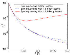
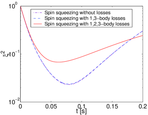
Figure 6: Spin squeezing with and without losses in a bimodal Rb condensate from the stationary two-mode model. A Feshbach resonance is used to reduce the inter-species scattering length. Violet dash-dotted line: without losses. Blue dashed line: with one and three-body losses. Red solid line: with one, two and three-body losses. (Top) with a $50-50$ mixing of the two states: $\bar{N}_{a}=\bar{N}_{b}=10^{4}$, $\chi=5.367\times 10^{-3}$s^-1, $\tilde{\chi}=5.412\times 10^{-4}$s^-1. (Bottom) in breathe-together conditions: $\bar{N}_{a}=7432$, $\bar{N}_{b}=12568$, $\chi=5.392\times 10^{-3}$s^-1, $\tilde{\chi}=1.386\times 10^{-3}$s^-1. Other parameters: $\omega=2\pi\times 42.6$ Hz, $m$=87 a.m.u., $a_{aa}=100.44\,r_{B}$, $a_{bb}=95.47\,r_{B}$, $a_{ab}=88.28\,r_{B}$, $r_{B}$ is the Bohr radius. Particle losses: $K_{1}^{(a)}=K_{1}^{(b)}=0.01$s^-1, $K_{2}^{(a)}=0$, $K_{2}^{(b)}=119\times 10^{-21}$m³s^-1Hall , $K_{2}^{(ab)}=78\times 10^{-21}$m³s^-1Note_2Bab , $K_{3}^{(a)}=6\times 10^{-42}$m⁶s^-1 Cornell97 .

4.2 Bimodal BEC of Na atoms

By using two states in the lower hyperfine manifold, one can greatly reduce two body losses. A possible example is of using Na atoms in the $|F=1,m_{F}=\pm 1\rangle$ states Nature . In Fig.7 we calculate the best obtainable squeezing with these two states. Parameters are chosen according to our optimization procedure of Section 3.2. A large amount of squeezing $\xi^{2}=1.9\times 10^{-3}$ can be reached at the best squeezing time.

Using our full numerical and our approximated dynamical approaches, (not shown) we checked that the two-mode model is an excellent approximation for these parameters.

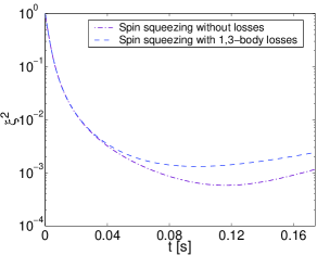
Figure 7: Spin squeezing with and without losses in a bimodal Na condensate from the stationary two-mode model. Violet dash-dotted line: without losses. Blue dashed line: with one and three-body losses. Optimized parameters: $\bar{N}_{a}=\bar{N}_{b}=4\times 10^{4}$ $\omega=2\pi\times 183$ Hz, $m$=23 a.m.u., $a_{aa}=a_{bb}=51.89\,r_{B}$, $a_{ab}=48.25\,r_{B}$, $r_{B}$ is the Bohr radius. $\chi=5.517\times 10^{-3}$s^-1, $\tilde{\chi}=0$. Particle losses: $K_{1}^{(a)}=K_{1}^{(b)}=0.01$s^-1, $K_{2}^{(a)}=K_{2}^{(b)}=0$, $K_{3}^{(a)}=K_{3}^{(b)}=2\times 10^{-42}$m⁶s^-1 3BNa .

5 Dynamically separated Rb BEC

In this subsection we consider a bimodal Rb condensate in $|F=1,m_{F}=-1\rangle$ and $|F=2,m_{F}=1\rangle$ states. Rather than using a Feshbach resonance to change $g_{ab}$, we consider the possibility of suddenly separating the two clouds right after the mixing $\pi/2$ pulse using state-selective potentials Munich , and recombining them after a well chosen interaction time. A related scheme using Bragg pulses in the frame of atom interferometry was proposed in Uffe . We consider disc shaped identical traps for the two states $a$ and $b$ with $\omega_{z}>\omega_{x,y}\equiv\omega_{\perp}$, that can be displaced independently along the $z$ axes. In order to minimize center-of-mass excitation of the cloud, we use a triangular ramp for the displacement velocity, as shown in Fig.8 (Bottom), with total move-out time $2\tau=4\pi/\omega_{z}$ David . In Fig.8 (Top) we show the $z$-dependence of densities of the clouds, integrated in the perpendicular $xy$ plane, as the clouds are separated and put back together after a given interaction time.

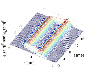
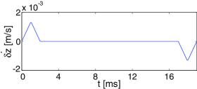
Figure 8: (Top) $|\phi_{a}(z,t)|^{2}$ and $|\phi_{b}(z,t)|^{2}$ in arbitrary units as the clouds are separated and put back together after an interaction time of about 15 ms. The harmonic potential for the $a$-component does not move, while that for the $b$-component is shifted vertically with a speed $\dot{\delta z}$. The distance between the two trap centers when they are separated is $\delta z=4\sqrt{\hbar/M\omega_{z}}$. (Bottom) variation in time of $\dot{\delta z}$. Parameters: $\bar{N}_{a}=\bar{N}_{b}=5\times 10^{4}$, $\omega_{x,y}=2\pi\times 2.31$ Hz, $\omega_{z}=2\pi\times 1$ kHz, $m$=87 a.m.u., $a_{aa}=100.44\,r_{B}$, $a_{bb}=95.47\,r_{B}$, $a_{ab}=98.09\,r_{B}$, $r_{B}$ is the Bohr radius. No particle losses.

We use our dynamical modulus-phase model in 3 dimensions to calculate the spin squeezing in this scheme. As the spatial overlap between the two clouds reduces a lot as they are separated, in Fig.9 we calculate both the spin squeezing obtained from the definitions (10)-(12) of spin operators (dashed line), and the “extracted spin squeezing” introduced in Section 2.5 based on the “instantaneous modes” (42)-(43) (solid line). The oscillations in the dashed line are due to tiny residual center of mass oscillations of the clouds that change periodically the small overlap between the two modes. They are absent in the extracted spin squeezing curve (solid line) as they do not affect the spin dynamics. When the clouds are put back together and the overlap between the modes is large again, the spin squeezing and the extracted spin squeezing curves give close results (not identical as the overlap of the two clouds is not precisely one).

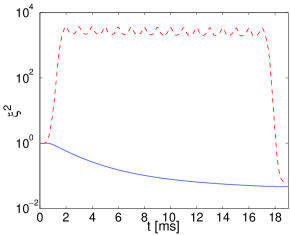
Figure 9: Spin squeezing as the two Rb condensates are separated and put back together after an interaction time of about 15 ms. Red dashed line: Spin squeezing obtained from the definitions (10)-(12) of the spin operators explicitly including the overlap between the clouds. Blue solid line: extracted spin squeezing based of the “instantaneous modes” (42)-(43). Parameters as in Fig.8.

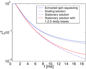
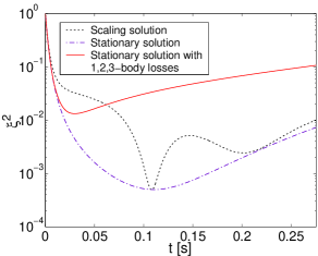
Figure 10: Spin squeezing as a function of time. (Top) comparison between a dynamical calculation and a stationary calculation. Blue solid line: extracted spin squeezing in 3D. Black doted line: 2D scaling solution based on (91). Violet dash-dotted line: stationary calculation in 3D without losses. Red solid line: stationary calculation in 3D with losses. Spin squeezing progresses more slowly in the dynamical calculation than in the stationary calculation. (Bottom) long time behavior. Black doted line: scaling solution. Violet dash-dotted line: stationary calculation without losses. Red solid line: stationary calculation with losses. Parameters: $\chi=5.003\times 10^{-3}$s^-1, $\tilde{\chi}=1.342\times 10^{-4}$s^-1, $K_{1}^{(a)}=K_{1}^{(b)}=0.01$s^-1, $K_{2}^{(a)}=0$, $K_{2}^{(b)}=119\times 10^{-21}$m³s^-1Hall , $K_{3}^{(a)}=6\times 10^{-42}$m⁶s^-1 Cornell97 . The other parameters are as in Fig.8.

In Fig.10 (Top) we compare the extracted spin squeezing curve of Fig.9 (solid line) with a two-mode stationary calculation (dash-dotted line) assuming stationary condensates in separated wells. We notice that the squeezing progresses much more slowly in the dynamical case. Indeed when we separate the clouds, the mean field changes suddenly for each component exciting a breathing mode whose amplitude and frequency is different for each of the Fock states involved. In the quasi 2D configuration considered here, the breathing of the wave functions is well described by a scaling solution in 2D for each condensate separately Scaling1 ; Scaling2 adapted to the case in which the trap frequency is not changed, but the mean-field is changed suddenly after separating the two internal states:

$${\phi}_{\varepsilon}(\vec{r}_{\perp},t)=\frac{e^{-i\eta_{\varepsilon}(t)}}{{\cal L}_{\varepsilon}(t)}e^{imr_{\perp}^{2}\dot{\cal L}_{\varepsilon}(t)/2\hbar{\cal L}_{\varepsilon}(t)}{\phi}_{0}\left(\frac{\vec{r}_{\perp}}{{\cal L}_{\varepsilon}(t)\,}\right)$$ (89)

with

$$\dot{\eta}_{\varepsilon} = \frac{\tilde{g}_{\varepsilon\varepsilon}}{\tilde{g}_{aa}}\,\frac{\bar{\mu}}{{\cal L}_{\varepsilon}^{2}\hbar}$$ (90)

$$\frac{d^{2}{\cal L}_{\varepsilon}}{dt^{2}} = \frac{N_{\varepsilon}}{N}\,\frac{\tilde{g}_{\varepsilon\varepsilon}}{\tilde{g}_{aa}}\,\frac{\omega_{\perp}^{2}}{{\cal L}_{\varepsilon}^{3}}-\omega_{\perp}^{2}{\cal L}_{\varepsilon}\>;$$ (91)

$${\phi}_{0}(\vec{r}_{\perp}) = \left(\frac{2}{\pi R_{0}^{2}}\right)^{1/2}\left[1-\frac{r_{\perp}^{2}}{R_{0}^{2}}\right]^{1/2}\,.$$ (92)

$\bar{\mu}$ is the chemical potential of the stationary condensate before the $\pi/2$ pulse, when all the $N$ atoms are in state $a$, $R_{0}=\sqrt{2\bar{\mu}/m\omega_{\perp}^{2}}$ is the corresponding Thomas-Fermi radius, and $\tilde{g}_{\varepsilon\varepsilon}$ is a reduced coupling constant to describe the interaction between two atoms in the $\varepsilon$ condensate in quasi 2D system, where we assume that the condensate wave functions in the confined direction are Gaussians:

$$\tilde{g}_{\varepsilon\varepsilon}=\frac{4\pi\hbar^{2}a_{\varepsilon\varepsilon}}{M}\sqrt{\frac{M\omega_{z}}{2\pi\hbar}}$$ (93)

with $a_{\varepsilon\varepsilon}$ the 3D scattering length. The initial conditions for (91) are ${\cal L}_{\varepsilon}(0)=1$ and $\dot{\cal L}_{\varepsilon}(0)=0$.

We can use (89) to calculate the squeezing (dotted curve) and we note that it reproduces well the spin squeezing curve obtained integrating 5 Gross-Pitaevskii equations in 3D (full line). As we studied in detail in Section 2.4, oscillations of the wave functions cause oscillations of the squeezing parameter due to entanglement between spatial and spin dynamics. Indeed what we see in the extracted spin squeezing curve of Fig.10 (Top) is the beginning of a slow oscillation for the squeezing parameter. In Fig.10 (Bottom) we show the long time behavior. There are indeed times at which the spatial and spin dynamics disentangle, and the dynamical curve and the steady state curve touch (see Sect. 2.4). Unfortunately these times are not accessible here in presence of losses (in particular the high two-body losses in the higher hyperfine state). Notice that in the first 15 ms of evolution considered in Fig.9 and Fig.10 (Top) the effect of losses is small and the main limitation at short times is provided by the spatial dynamics.

For a lower number of atoms, the sudden change in the mean field and the consequent oscillations of the squeezing parameter are reduced. In Fig.11 we show the spin squeezing obtained by suddenly separating two BEC of Rb atoms in $|F=1,m_{F}=-1\rangle$ and $|F=2,m_{F}=1\rangle$ states with 1000 atoms in each component. The dotted line is a dynamical calculation using the quasi 2D scaling solution (91) (and no losses), while the dash-dotted line and the solid line are stationary calculations without and with losses respectively. Note that around $t=0.02$s, where the dynamical curve and the stationary curve touch, a squeezing of about $\xi^{2}\sim 2\times 10^{-2}$ could be reached despite the high losses in the $F=2$ state NotePhil .

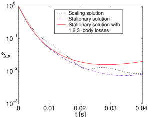
Figure 11: Spin squeezing as a function of time in two small Rb condensates. Black doted line: scaling solution based on (91). Violet dash-dotted line: stationary calculation without losses. Red solid line: stationary calculation with losses. Parameters: $K_{1}^{(a)}=K_{1}^{(b)}=0.01$s^-1, $K_{2}^{(a)}=0$, $K_{2}^{(b)}=119\times 10^{-21}$m³s^-1Hall , $K_{3}^{(a)}=6\times 10^{-42}$m⁶s^-1 Cornell97 . The other parameters: $\bar{N}_{a}=\bar{N}_{b}=10^{3}$, $\omega_{x,y}=2\pi\times 11.82$ Hz, $\omega_{z}=2\pi\times 2$ kHz, $m$=87 a.m.u., $a_{aa}=100.44\,r_{B}$, $a_{bb}=95.47\,r_{B}$, $a_{ab}=98.09\,r_{B}$, $r_{B}$ is the Bohr radius. $\chi=0.213$s^-1, $\tilde{\chi}=2.763\times 10^{-3}$s^-1.

6 Conclusions

In conclusion we developed a method to study the entangled spatial and spin dynamics in binary mixtures of Bose-Einstein condensates. The method, which is the natural extension of our work EPJD to the case of spin squeezing, allows a full analytical treatment in some cases and can be used in the general case to study a priori complicated situations in 3D without the need of heavy numerics. Including the effect of particle losses and spatial dynamics, we have calculated the maximum squeezing obtainable in a bimodal condensate of Na atoms in $|F=1,m_{F}=\pm 1\rangle$ states when the two condensates overlap in space, and we have calculated the squeezing in a bimodal Rb condensate in which a Feshbach resonance is used to reduce the inter-species scattering length as recently realized experimentally Widera . For Rb we also propose an original scheme in which the two components are spatially separated using state-dependent potentials, recently realized for the $|F=1,m_{F}=-1\rangle$ and $|F=2,m_{F}=1\rangle$ states, and then recombined after a well chosen squeezing time. With this method we show that $\xi^{2}\sim 2\times 10^{-2}$ could be reached in condensates of 1000 atoms, despite the high two-body losses in the higher hyperfine state.

Yun Li acknowledges support from the ENS-ECNU program, and A.S. acknowledges stimulating discussions with M. Oberthaler, J. Estève and K. Mølmer. Our group is a member of IFRAF.

Appendix A Quantum averages of the field operators

Using equations (2.2)-(21), the averages needed to calculate squeezing parameter can be written in terms of the wave functions $\phi_{a}$, $\phi_{b}$ and the phase factor $A$ solution of equation (9):

$$\langle\hat{\psi}_{b}^{\dagger}(\vec{r})\hat{\psi}_{a}(\vec{r})\rangle$$ (94)

$$= \sum^{N}_{N_{a}=1}\frac{N!}{(N_{a}-1)!N_{b}!}|C_{a}|^{2(N_{a}-1)}|C_{b}|^{2N_{b}}C^{\ast}_{b}C_{a}$$

$$\times\phi^{\ast}_{b}(N_{a}-1,N_{b}+1,\vec{r})\phi_{a}(N_{a},N_{b},\vec{r})$$

$$\times\exp\{i[A(N_{a}-1,N_{b}+1)-A(N_{a},N_{b})]/\hbar\}$$

$$\times[\langle\phi_{a}(N_{a}-1,N_{b}+1)|\phi_{a}(N_{a},N_{b})\rangle]^{N_{a}-1}$$

$$\times[\langle\phi_{b}(N_{a}-1,N_{b}+1)|\phi_{b}(N_{a},N_{b})\rangle]^{N_{b}}\,.$$

$$\langle\hat{\psi}_{b}^{\dagger}(\vec{r})\hat{\psi}_{a}^{\dagger}(\vec{r}^{\prime})\hat{\psi}_{a}(\vec{r})\hat{\psi}_{b}(\vec{r}^{\prime})\rangle$$ (95)

$$= \sum^{N-1}_{N_{a}=1}\frac{N!}{(N_{a}-1)!(N_{b}-1)!}|C_{a}|^{2N_{a}}|C_{b}|^{2N_{b}}$$

$$\times\phi^{\ast}_{b}(N_{a},N_{b},\vec{r})\phi^{\ast}_{a}(N_{a},N_{b},\vec{r}^{\prime})\phi_{a}(N_{a},N_{b},\vec{r})$$

$$\times\phi_{b}(N_{a},N_{b},\vec{r}^{\prime})\,.$$

$$\langle\hat{\psi}_{b}^{\dagger}(\vec{r})\hat{\psi}_{b}^{\dagger}(\vec{r}^{\prime})\hat{\psi}_{a}(\vec{r})\hat{\psi}_{a}(\vec{r}^{\prime})\rangle$$ (96)

$$= \sum^{N}_{N_{a}=2}\frac{N!}{(N_{a}-2)!N_{b}!}|C_{a}|^{2(N_{a}-2)}|C_{b}|^{2N_{b}}C^{\ast 2}_{b}C_{a}^{2}$$

$$\times\phi^{\ast}_{b}(N_{a}-2,N_{b}+2,\vec{r})\phi^{\ast}_{b}(N_{a}-2,N_{b}+2,\vec{r}^{\prime})$$

$$\times\phi_{a}(N_{a},N_{b},\vec{r})\phi_{a}(N_{a},N_{b},\vec{r}^{\prime})$$

$$\times\exp\{i[A(N_{a}-2,N_{b}+2)-A(N_{a},N_{b})]/\hbar\}$$

$$\times[\langle\phi_{a}(N_{a}-2,N_{b}+2)|\phi_{a}(N_{a},N_{b})\rangle]^{N_{a}-2}$$

$$\times[\langle\phi_{b}(N_{a}-2,N_{b}+2)|\phi_{b}(N_{a},N_{b})\rangle]^{N_{b}}\,.$$

$$\langle\hat{\psi}_{b}^{\dagger}(\vec{r})\hat{\psi}_{b}^{\dagger}(\vec{r}^{\prime})\hat{\psi}_{b}(\vec{r})\hat{\psi}_{a}(\vec{r}^{\prime})\rangle$$ (97)

$$= \sum^{N-1}_{N_{a}=1}\frac{N!}{(N_{a}-1)!(N_{b}-1)!}|C_{a}|^{2(N_{a}-1)}|C_{b}|^{2N_{b}}C^{\ast}_{b}C_{a}$$

$$\times\phi^{\ast}_{b}(N_{a}-1,N_{b}+1,\vec{r})\phi^{\ast}_{b}(N_{a}-1,N_{b}+1,\vec{r}^{\prime})$$

$$\times\phi_{b}(N_{a},N_{b},\vec{r})\phi_{a}(N_{a},N_{b},\vec{r}^{\prime})$$

$$\times\exp\{i[A(N_{a}-1,N_{b}+1)-A(N_{a},N_{b})]/\hbar\}$$

$$\times[\langle\phi_{a}(N_{a}-1,N_{b}+1)|\phi_{a}(N_{a},N_{b})\rangle]^{N_{a}-1}$$

$$\times[\langle\phi_{b}(N_{a}-1,N_{b}+1)|\phi_{b}(N_{a},N_{b})\rangle]^{N_{b}-1}\,.$$

$$\langle\hat{\psi}_{a}^{\dagger}(\vec{r})\hat{\psi}_{a}^{\dagger}(\vec{r}^{\prime})\hat{\psi}_{a}(\vec{r})\hat{\psi}_{b}(\vec{r}^{\prime})\rangle$$ (98)

$$= \sum^{N-1}_{N_{a}=1}\frac{N!}{(N_{a}-1)!(N_{b}-1)!}|C_{a}|^{2N_{a}}|C_{b}|^{2(N_{b}-1)}C^{\ast}_{a}C_{b}$$

$$\times\phi^{\ast}_{a}(N_{a}+1,N_{b}-1,\vec{r})\phi^{\ast}_{a}(N_{a}+1,N_{b}-1,\vec{r}^{\prime})$$

$$\times\phi_{a}(N_{a},N_{b},\vec{r})\phi_{b}(N_{a},N_{b},\vec{r}^{\prime})$$

$$\times\exp\{i[A(N_{a}+1,N_{b}-1)-A(N_{a},N_{b})]/\hbar\}$$

$$\times[\langle\phi_{a}(N_{a}+1,N_{b}-1)|\phi_{a}(N_{a},N_{b})\rangle]^{N_{a}-1}$$

$$\times[\langle\phi_{b}(N_{a}+1,N_{b}-1)|\phi_{b}(N_{a},N_{b})\rangle]^{N_{b}-1}\,.$$

We use these averages to calculate the squeezing in our full dynamical model. In practice we do not sum over all the Fock states but over a “large enough width” (typically $>6\sqrt{N}$) around the average number of atoms $\bar{N}_{a}$, $\bar{N}_{b}$. The spin squeezing is obtained by equation (15) using the definitions (10)-(12) for the spin operators.

Appendix B Quantum averages in the modulus-phase approach

Within the modulus-phase approximation, the scalar product of the wave vectors can be written as

$$\langle\phi_{a}(N_{a}-\beta,N_{b}+\beta)|\phi_{a}(N_{a},N_{b})\rangle$$

$$= \exp\{i\beta\textstyle\int d^{3}r|\bar{\phi}_{a}(\vec{r})|^{2}[\chi_{0}(\vec{r})+\chi_{d}(\vec{r})]\}\;\;$$

$$\langle\phi_{b}(N_{a}-\beta,N_{b}+\beta)|\phi_{b}(N_{a},N_{b})\rangle$$

$$= \exp\{i\beta\textstyle\int d^{3}r|\bar{\phi}_{b}(\vec{r})|^{2}[\chi_{0}(\vec{r})-\chi_{d}(\vec{r})]\}\;\;$$ (102)

$$\langle\phi_{b}(N_{a}-\beta,N_{b}+\beta)|\phi_{a}(N_{a},N_{b})\rangle$$

$$= \textstyle\int d^{3}r\bar{\phi}^{\ast}_{b}(\vec{r})\bar{\phi}_{a}(\vec{r})\exp[i(N_{a}-\beta)\chi_{d}(\vec{r})-iN_{b}\chi_{d}(\vec{r})]$$

$$\times\exp[i(N-\bar{N})\chi_{s}(\vec{r})-iN(|C_{a}|^{2}-|C_{b}|^{2})\chi_{d}(\vec{r})]$$

$$\times\exp[i\beta\chi_{0}(\vec{r})]$$

$$\langle\phi_{a}(N_{a}+\beta,N_{b}-\beta)|\phi_{b}(N_{a},N_{b})\rangle$$

$$= \textstyle\int d^{3}r\bar{\phi}^{\ast}_{a}(\vec{r})\bar{\phi}_{b}(\vec{r})\exp[-iN_{a}\chi_{d}(\vec{r})+i(N_{b}-\beta)\chi_{d}(\vec{r})]$$

$$\times\exp[-i(N-\bar{N})\chi_{s}(\vec{r})-iN(|C_{a}|^{2}-|C_{b}|^{2})\chi_{d}(\vec{r})]$$

$$\times\exp[-i\beta\chi_{0}(\vec{r})]$$

where $\beta\in\mathbb{Z}$, and we have used the relation

$$\textstyle\int d^{3}r|\bar{\phi}_{\varepsilon}|^{2}\exp[i(\partial_{N_{a}}-\partial_{N_{b}})\theta_{\varepsilon}(\bar{N}_{a},\bar{N}_{b})]$$

$$\hskip 22.76219pt\simeq\exp[\,i\textstyle\int d^{3}r|\bar{\phi}_{\varepsilon}|^{2}(\partial_{N_{a}}-\partial_{N_{b}})\theta_{\varepsilon}(\bar{N}_{a},\bar{N}_{b})]\,.\hskip 14.22636pt$$ (103)

By using the Gross-Pitaevskii equations (7) for $\phi_{\varepsilon}(N_{a},N_{b})$ and for $\phi_{\varepsilon}(\bar{N}_{a},\bar{N}_{b})$, one obtains

$$i\hbar\partial_{t}\left[(N_{a}-\bar{N}_{a})\frac{\partial\theta_{\varepsilon}}{\partial N_{a}}+(N_{b}-\bar{N}_{b})\frac{\partial\theta_{\varepsilon}}{\partial N_{b}}\right]_{\bar{N}_{a},\bar{N}_{b}}$$

$$\hskip 14.22636pt=(N_{\varepsilon}-\bar{N}_{\varepsilon})g_{\varepsilon\varepsilon}|\phi_{\varepsilon}|^{2}+(N_{\varepsilon^{\prime}}-\bar{N}_{\varepsilon^{\prime}})g_{\varepsilon\varepsilon^{\prime}}|\phi_{\varepsilon^{\prime}}|^{2}\,,\hskip 22.76219pt$$ (104)

where $\varepsilon\neq\varepsilon^{\prime}=a,b$. Using (104) together with the initial condition (8), we obtain for the phase factor $A$ in Eq. (9)

$$[A(N_{a}-1,N_{b}+1)-A(N_{a},N_{b})]/\hbar$$

$$= -(N_{a}-1)\textstyle\int d^{3}r|\bar{\phi}_{a}(\vec{r})|^{2}[\chi_{0}(\vec{r})+\chi_{d}(\vec{r})]$$

$$-N_{b}\textstyle\int d^{3}r|\bar{\phi}_{b}(\vec{r})|^{2}[\chi_{0}(\vec{r})-\chi_{d}(\vec{r})]$$

$$[A(N_{a}-2,N_{b}+2)-A(N_{a},N_{b})]/\hbar$$

$$= -2(N_{a}-2)\textstyle\int d^{3}r|\bar{\phi}_{a}(\vec{r})|^{2}[\chi_{0}(\vec{r})+\chi_{d}(\vec{r})]$$ (106)

$$-2N_{b}\textstyle\int d^{3}r|\bar{\phi}_{b}(\vec{r})|^{2}[\chi_{0}(\vec{r})-\chi_{d}(\vec{r})]$$

$$-\textstyle\int d^{3}r\{|\bar{\phi}_{a}(\vec{r})|^{2}[\chi_{0}(\vec{r})+\chi_{d}(\vec{r})]$$

$$+|\bar{\phi}_{b}(\vec{r})|^{2}[\chi_{0}(\vec{r})-\chi_{d}(\vec{r})]\}$$

The averages and variances of the spin operators equations (10)-(12) are obtained by equations (94)-(98) after spatial integration. We get:

$$\textstyle\int d^{3}r\langle\hat{\psi}_{b}^{\dagger}(\vec{r})\hat{\psi}_{a}(\vec{r})\rangle$$ (111)

$$= NC^{\ast}_{b}C_{a}\textstyle\int d^{3}r\bar{\phi}^{\ast}_{b}(\vec{r})\bar{\phi}_{a}(\vec{r})[|C_{a}|^{2}e^{i\chi_{d}(\vec{r})}+|C_{b}|^{2}e^{-i\chi_{d}(\vec{r})}]^{N-1}$$

$$\times\exp[i(N-\bar{N})\chi_{s}(\vec{r})]\exp[-i\bar{N}(|C_{a}|^{2}-|C_{b}|^{2})\chi_{d}(\vec{r})]$$

$$\times\exp[i\chi_{0}(\vec{r})]\,.$$

$$\textstyle\int d^{3}rd^{3}r^{\prime}\langle\hat{\psi}_{b}^{\dagger}(\vec{r})\hat{\psi}_{a}^{\dagger}(\vec{r}^{\prime})\hat{\psi}_{a}(\vec{r})\hat{\psi}_{b}(\vec{r}^{\prime})\rangle$$

$$= N(N-1)|C_{a}|^{2}|C_{b}|^{2}\textstyle\int d^{3}rd^{3}r^{\prime}\bar{\phi}^{\ast}_{b}(\vec{r})\bar{\phi}_{a}(\vec{r})\bar{\phi}^{\ast}_{a}(\vec{r}^{\prime})\bar{\phi}_{b}(\vec{r}^{\prime})\,.$$

$$\textstyle\int d^{3}rd^{3}r^{\prime}\langle\hat{\psi}_{b}^{\dagger}(\vec{r})\hat{\psi}_{b}^{\dagger}(\vec{r}^{\prime})\hat{\psi}_{a}(\vec{r})\hat{\psi}_{a}(\vec{r}^{\prime})\rangle$$

$$= N(N-1)C^{\ast 2}_{b}C^{2}_{a}\textstyle\int d^{3}rd^{3}r^{\prime}\bar{\phi}^{\ast}_{b}(\vec{r})\bar{\phi}_{a}(\vec{r})\bar{\phi}^{\ast}_{b}(\vec{r}^{\prime})\bar{\phi}_{a}(\vec{r}^{\prime})$$

$$\times[|C_{a}|^{2}e^{i\chi_{d}(\vec{r})+i\chi_{d}(\vec{r}^{\prime})}+|C_{b}|^{2}e^{-i\chi_{d}(\vec{r})-i\chi_{d}(\vec{r}^{\prime})}]^{N-2}$$

$$\times\exp\{-i\bar{N}(|C_{a}|^{2}-|C_{b}|^{2})[\chi_{d}(\vec{r})+\chi_{d}(\vec{r}^{\prime})]\}\exp\{2i[\chi_{0}(\vec{r})$$

$$+\chi_{0}(\vec{r}^{\prime})]\}\exp\{i(N-\bar{N})[\chi_{s}(\vec{r})+\chi_{s}(\vec{r}^{\prime})]\}$$

$$\times\exp\{-i\textstyle\int d^{3}r^{\prime\prime}(|\bar{\phi}_{a}|^{2}[\chi_{0}(\vec{r}^{\prime\prime})+\chi_{d}(\vec{r}^{\prime\prime})]$$

$$+|\bar{\phi}_{b}|^{2}[\chi_{0}(\vec{r}^{\prime\prime})-\chi_{d}(\vec{r}^{\prime\prime})])\}\,.$$

$$\textstyle\int d^{3}rd^{3}r^{\prime}\langle\hat{\psi}_{b}^{\dagger}(\vec{r})\hat{\psi}_{b}^{\dagger}(\vec{r}^{\prime})\hat{\psi}_{b}(\vec{r})\hat{\psi}_{a}(\vec{r}^{\prime})\rangle$$

$$= N(N-1)C^{\ast}_{b}C_{a}|C_{b}|^{2}\textstyle\int d^{3}r^{\prime}\bar{\phi}^{\ast}_{b}(\vec{r}^{\prime})\bar{\phi}_{a}(\vec{r}^{\prime})[|C_{a}|^{2}e^{i\chi_{d}(\vec{r}^{\prime})}$$

$$+|C_{b}|^{2}e^{-i\chi_{d}(\vec{r}^{\prime})}]^{N-2}\exp[-i\bar{N}(|C_{a}|^{2}-|C_{b}|^{2})\chi_{d}(\vec{r}^{\prime})]$$

$$\times\exp[i\chi_{0}(\vec{r}^{\prime})-i\chi_{d}(\vec{r}^{\prime})]\exp[i(N-\bar{N})\chi_{s}(\vec{r}^{\prime})]\,.$$

$$\textstyle\int d^{3}rd^{3}r^{\prime}\langle\hat{\psi}_{a}^{\dagger}(\vec{r})\hat{\psi}_{a}^{\dagger}(\vec{r}^{\prime})\hat{\psi}_{a}(\vec{r})\hat{\psi}_{b}(\vec{r}^{\prime})\rangle$$

$$= N(N-1)C^{\ast}_{a}C_{b}|C_{a}|^{2}\textstyle\int d^{3}r^{\prime}\bar{\phi}^{\ast}_{a}(\vec{r}^{\prime})\bar{\phi}_{b}(\vec{r}^{\prime})[|C_{a}|^{2}e^{-i\chi_{d}(\vec{r}^{\prime})}$$

$$+|C_{b}|^{2}e^{i\chi_{d}(\vec{r}^{\prime})}]^{N-2}\exp[i\bar{N}(|C_{a}|^{2}-|C_{b}|^{2})\chi_{d}(\vec{r}^{\prime})]$$

$$\times\exp[-i\chi_{0}(\vec{r}^{\prime})-i\chi_{d}(\vec{r}^{\prime})]\exp[-i(N-\bar{N})\chi_{s}(\vec{r}^{\prime})]\,.$$

In the above expressions $\chi_{d}$, $\chi_{s}$ and $\chi_{0}$ are the space and time dependent functions defined in equations (24), (25) and (26). In practice it is sufficient to evolve five wave functions $\phi_{a}(\vec{r},t)$, $\phi_{b}(\vec{r},t)$ for ($\bar{N}_{a},\bar{N}_{b}\pm\delta N_{b}$) and ($\bar{N}_{a}\pm\delta N_{a},\bar{N}_{b}$) with $\delta N_{a,b}\neq 0$ (to calculate numerically $\chi_{d}$ $\chi_{s}$ $\chi_{0}$), and with $\delta N_{a,b}=0$ (to calculate the central wave functions $\bar{\phi}_{a,b}$). The spin squeezing is obtained by equation (15) using the definitions (10)-(12) for the spin operators.

Appendix C Equality of $\chi_{s}$ and $\chi_{0}$ in the breathe-together configuration

Evaluating (104) for $\varepsilon=a$, $N_{a}=\bar{N}_{a}$; $\varepsilon=b$, $N_{b}=\bar{N}_{b}$ and subtracting the two relations, on obtains

$$\partial_{t}\left(\bar{\frac{\partial\theta_{a}}{\partial N_{b}}}-\bar{\frac{\partial\theta_{b}}{\partial N_{a}}}\right)=0$$ (112)

where we used the fact that in breathe-together conditions $|\bar{\phi}_{a}|=|\bar{\phi}_{b}|$. Equation (112) implies that the time derivative of $\chi_{s}-\chi_{0}$ is zero. As for $t=0$ $\chi_{s}=\chi_{0}=0$, we conclude that $\chi_{s}=\chi_{0}$ at all times.

Appendix D Extracted spin squeezing quantum averages

By using the instantaneous modes (42)-(43) and within the modulus-phase approach, the quantum averages useful to calculate spin squeezing are expressed in terms of the functions:

$$\chi^{\text{ex}}_{d}(\vec{r},\vec{r}^{\prime}) = \frac{1}{2}(\partial_{N_{a}}-\partial_{N_{b}})[\theta_{a}(\vec{r})-\theta_{b}(\vec{r}^{\prime})](\bar{N}_{a},\bar{N}_{b})$$ (113)

$$\chi^{\text{ex}}_{s}(\vec{r},\vec{r}^{\prime}) = \frac{1}{2}(\partial_{N_{a}}+\partial_{N_{b}})[\theta_{a}(\vec{r})-\theta_{b}(\vec{r}^{\prime})](\bar{N}_{a},\bar{N}_{b})$$ (114)

$$\chi^{\text{ex}}_{0}(\vec{r},\vec{r}^{\prime}) = \frac{1}{2}(\partial_{N_{a}}-\partial_{N_{b}})[\theta_{a}(\vec{r})+\theta_{b}(\vec{r}^{\prime})](\bar{N}_{a},\bar{N}_{b})\,.\hskip 17.07164pt$$ (115)

We obtain:

$$\langle\tilde{b}^{\dagger}\tilde{a}\rangle = NC^{\ast}_{b}C_{a}\textstyle\int d^{3}r_{1}d^{3}r_{2}|\bar{\phi}_{b}(\vec{r}_{1})|^{2}|\bar{\phi}_{a}(\vec{r}_{2})|^{2}$$ (116)

$$\times[|C_{a}|^{2}e^{i\chi^{\text{ex}}_{d}(\vec{r}_{2},\vec{r}_{1})}+|C_{b}|^{2}e^{-i\chi^{\text{ex}}_{d}(\vec{r}_{2},\vec{r}_{1})}]^{N-1}$$

$$\times\exp[i(N-\bar{N})\chi^{\text{ex}}_{s}(\vec{r}_{2},\vec{r}_{1})+i\chi^{\text{ex}}_{0}(\vec{r}_{2},\vec{r}_{1})]$$

$$\times\exp[-i\bar{N}(|C_{a}|^{2}-|C_{b}|^{2})\chi^{\text{ex}}_{d}(\vec{r}_{2},\vec{r}_{1})]$$

$$\langle\tilde{b}^{\dagger}\tilde{a}^{\dagger}\tilde{a}\tilde{b}\rangle = N(N-1)|C_{a}|^{2}|C_{b}|^{2}$$ (117)

$$\langle\tilde{b}^{\dagger}\tilde{b}^{\dagger}\tilde{a}\tilde{a}\rangle = N(N-1)C^{\ast 2}_{b}C^{2}_{a}\textstyle\int d^{3}r_{1}d^{3}r_{2}d^{3}r_{3}d^{3}r_{4}$$ (118)

$$\times|\bar{\phi}_{b}(\vec{r}_{1})|^{2}|\bar{\phi}_{b}(\vec{r}_{2})|^{2}|\bar{\phi}_{a}(\vec{r}_{3})|^{2}|\bar{\phi}_{a}(\vec{r}_{4})|^{2}$$

$$\times\{|C_{a}|^{2}e^{i[\chi^{\text{ex}}_{d}(\vec{r}_{4},\vec{r}_{2})+\chi^{\text{ex}}_{d}(\vec{r}_{3},\vec{r}_{1})]}$$

$$+|C_{b}|^{2}e^{-i[\chi^{\text{ex}}_{d}(\vec{r}_{4},\vec{r}_{2})+\chi^{\text{ex}}_{d}(\vec{r}_{3},\vec{r}_{1})]}\}^{N-2}$$

$$\times\exp\{2i[\chi^{\text{ex}}_{0}(\vec{r}_{4},\vec{r}_{2})+\chi^{\text{ex}}_{0}(\vec{r}_{3},\vec{r}_{1})]\}$$

$$\times\exp\{-i\bar{N}(|C_{a}|^{2}-|C_{b}|^{2})[\chi^{\text{ex}}_{d}(\vec{r}_{4},\vec{r}_{2})+\chi^{\text{ex}}_{d}(\vec{r}_{3},\vec{r}_{1})]\}$$

$$\times\exp\{i(N-\bar{N})[\chi^{\text{ex}}_{s}(\vec{r}_{4},\vec{r}_{2})+\chi^{\text{ex}}_{s}(\vec{r}_{3},\vec{r}_{1})]\}$$

$$\times\exp\{-i\textstyle\int d^{3}r_{5}(|\bar{\phi}_{a}(\vec{r}_{5})|^{2}[\chi^{\text{ex}}_{0}(\vec{r}_{5},\vec{r}_{5})+\chi^{\text{ex}}_{d}(\vec{r}_{5},\vec{r}_{5})]$$

$$+|\bar{\phi}_{b}(\vec{r}_{5})|^{2}[\chi^{\text{ex}}_{0}(\vec{r}_{5},\vec{r}_{5})-\chi^{\text{ex}}_{d}(\vec{r}_{5},\vec{r}_{5})])\}$$

$$\langle\tilde{b}^{\dagger}\tilde{b}^{\dagger}\tilde{b}\tilde{a}\rangle = N(N-1)C^{\ast}_{b}C_{a}|C_{b}|^{2}\textstyle\int d^{3}r_{1}d^{3}r_{2}|\bar{\phi}_{b}(\vec{r}_{1})|^{2}|\bar{\phi}_{a}(\vec{r}_{2})|^{2}$$ (119)

$$\times[|C_{a}|^{2}e^{i\chi^{\text{ex}}_{d}(\vec{r}_{2},\vec{r}_{1})}+|C_{b}|^{2}e^{-i\chi^{\text{ex}}_{d}(\vec{r}_{2},\vec{r}_{1})}]^{N-2}$$

$$\times\exp[i\chi^{\text{ex}}_{0}(\vec{r}_{2},\vec{r}_{1})-i\chi^{\text{ex}}_{d}(\vec{r}_{2},\vec{r}_{1})]$$

$$\times\exp[-i\bar{N}(|C_{a}|^{2}-|C_{b}|^{2})\chi^{\text{ex}}_{d}(\vec{r}_{2},\vec{r}_{1})]$$

$$\times\exp[i(N-\bar{N})\chi^{\text{ex}}_{s}(\vec{r}_{2},\vec{r}_{1})]$$

$$\langle\tilde{a}^{\dagger}\tilde{a}^{\dagger}\tilde{a}\tilde{b}\rangle = N(N-1)C^{\ast}_{a}C_{b}|C_{a}|^{2}\textstyle\int d^{3}r_{1}d^{3}r_{2}|\bar{\phi}_{a}(\vec{r}_{1})|^{2}|\bar{\phi}_{b}(\vec{r}_{2})|^{2}$$ (120)

$$\times[|C_{b}|^{2}e^{i\chi^{\text{ex}}_{d}(\vec{r}_{1},\vec{r}_{2})}+|C_{a}|^{2}e^{-i\chi^{\text{ex}}_{d}(\vec{r}_{1},\vec{r}_{2})}]^{N-2}$$

$$\times\exp[-i\chi^{\text{ex}}_{0}(\vec{r}_{1},\vec{r}_{2})-i\chi^{\text{ex}}_{d}(\vec{r}_{1},\vec{r}_{2})]$$

$$\times\exp[i\bar{N}(|C_{a}|^{2}-|C_{b}|^{2})\chi^{\text{ex}}_{d}(\vec{r}_{1},\vec{r}_{2})]$$

$$\times\exp[-i(N-\bar{N})\chi^{\text{ex}}_{s}(\vec{r}_{1},\vec{r}_{2})]$$

In case the wave functions $\bar{\phi}_{a}$, $\bar{\phi}_{b}$ are stationary we recover the stationary two-mode model averages given in the next appendix in the particular case of no losses. The spin squeezing is obtained by equation (15) using the definitions (44)-(46) for the spin operators.

Appendix E Quantum averages with one-body losses: Exact solution in the non symmetric case

In this appendix we give the exact result for quantum averages needed to calculate spin squeezing in the case of a two-mode model with one-body losses only, in the general non-symmetric case.

$$\langle a^{\dagger}a\rangle = |C_{a}|^{2}N\exp(-\gamma_{a}t)\phantom{\frac{1}{2}}$$ (121)

$$\langle a^{\dagger}a^{\dagger}aa\rangle = |C_{a}|^{4}N(N-1)\exp(-2\gamma_{a}t)\phantom{\frac{1}{2}}$$ (122)

$$\langle b^{\dagger}b^{\dagger}bb\rangle = |C_{b}|^{4}N(N-1)\exp(-2\gamma_{b}t)\phantom{\frac{1}{2}}$$ (123)

$$\langle b^{\dagger}a^{\dagger}ab\rangle = |C_{b}|^{2}|C_{a}|^{2}N(N-1)\exp[-(\gamma_{a}+\gamma_{b})t]\phantom{\frac{1}{2}}$$ (124)

$$\langle b^{\dagger}a\rangle = C^{\ast}_{b}C_{b}e^{-2ivt}N\exp\left[-\frac{1}{2}(\gamma_{a}+\gamma_{b})t\right]L_{1}^{N-1}\hskip 14.22636pt$$ (125)

$$\langle b^{\dagger}b^{\dagger}ba\rangle = |C_{b}|^{2}C^{\ast}_{b}C_{a}e^{-2ivt}N(N-1)e^{i\chi t}$$ (126)

$$\times \exp\left[-\frac{1}{2}(\gamma_{a}+3\gamma_{b})t\right]L_{1}^{N-2}$$

$$\langle a^{\dagger}a^{\dagger}ab\rangle = |C_{a}|^{2}C^{\ast}_{a}C_{b}e^{2ivt}N(N-1)e^{i\chi t}$$ (127)

$$\times \exp\left[-\frac{1}{2}(3\gamma_{a}+\gamma_{b})t\right]L_{-1}^{N-2}$$

$$\langle b^{\dagger}b^{\dagger}aa\rangle = C^{\ast 2}_{b}C^{2}_{a}e^{-4ivt}N(N-1)$$ (128)

$$\times \exp\left[-(\gamma_{a}+\gamma_{b})t\right]L_{2}^{N-2}\phantom{\frac{1}{2}}$$

where we introduced the function $L_{\beta}$ with $\beta=-1,1,2$

$$L_{\beta} = \frac{|C_{a}|^{2}}{\gamma_{a}+i\beta(\chi+\tilde{\chi})}\left[\gamma_{a}e^{i\beta\tilde{\chi}t}+i\beta(\chi+\tilde{\chi})e^{-(\gamma_{a}+i\beta\chi)t}\right]$$

$$+ \frac{|C_{b}|^{2}}{\gamma_{b}-i\beta(\chi-\tilde{\chi})}\left[\gamma_{b}e^{i\beta\tilde{\chi}t}-i\beta(\chi-\tilde{\chi})e^{-(\gamma_{b}-i\beta\chi)t}\right]$$

and $v$ given by (69).

Appendix F Quantum averages with one, two, three-body losses in the non-symmetric case

In this appendix we give the quantum averages useful to calculate spin squeezing for the two-mode model in the general non-symmetric case, in presence of one, two and three-body losses.

$$\langle a^{\dagger}a\rangle = |C_{a}|^{2}e^{-\lambda t}\left[N-(\partial_{\sigma_{1}}+\partial_{\sigma_{2}})\right]F_{0}(\sigma_{1},\sigma_{2})$$ (130)

$$\langle a^{\dagger}a^{\dagger}aa\rangle = |C_{a}|^{4}e^{-\lambda t}\left[N-(\partial_{\sigma_{1}}+\partial_{\sigma_{2}}-1)\right]$$ (131)

$$\times \left[N-(\partial_{\sigma_{1}}+\partial_{\sigma_{2}})\right]F_{0}(\sigma_{1},\sigma_{2})$$

$$\langle b^{\dagger}b^{\dagger}bb\rangle = |C_{b}|^{4}e^{-\lambda t}\left[N-(\partial_{\sigma_{1}}+\partial_{\sigma_{2}}-1)\right]$$ (132)

$$\times \left[N-(\partial_{\sigma_{1}}+\partial_{\sigma_{2}})\right]F_{0}(\sigma_{1},\sigma_{2})$$

$$\langle b^{\dagger}a^{\dagger}ab\rangle = |C_{b}|^{2}|C_{a}|^{2}e^{-\lambda t}\left[N-(\partial_{\sigma_{1}}+\partial_{\sigma_{2}}-1)\right]$$ (133)

$$\times \left[N-(\partial_{\sigma_{1}}+\partial_{\sigma_{2}})\right]F_{0}(\sigma_{1},\sigma_{2})$$

$$\langle b^{\dagger}a\rangle = C^{\ast}_{b}C_{b}e^{-(2iv+\lambda)t}\left(|C_{a}|^{2}e^{-i\chi t}+|C_{b}|^{2}e^{i\chi t}\right)^{N-1}$$ (134)

$$\times \left[N-(\partial_{\sigma_{1}}+\partial_{\sigma_{2}})\right]F_{1}(\sigma_{1},\sigma_{2})$$

$$\langle b^{\dagger}b^{\dagger}ba\rangle = |C_{b}|^{2}C^{\ast}_{b}C_{a}e^{-(2iv+\lambda)t}\left(|C_{a}|^{2}e^{-i\chi t}+|C_{b}|^{2}e^{i\chi t}\right)^{N-2}$$ (135)

$$\times e^{i\chi t}\left[N-(\partial_{\sigma_{1}}+\partial_{\sigma_{2}}-1)\right]\left[N-(\partial_{\sigma_{1}}+\partial_{\sigma_{2}})\right]$$

$$\times F_{1}(\sigma_{1},\sigma_{2})$$

$$\langle a^{\dagger}a^{\dagger}ab\rangle = |C_{a}|^{2}C^{\ast}_{a}C_{b}e^{(2iv-\lambda)t}\left(|C_{b}|^{2}e^{-i\chi t}+|C_{a}|^{2}e^{i\chi t}\right)^{N-2}$$ (136)

$$\times e^{i\chi t}\left[N-(\partial_{\sigma_{1}}+\partial_{\sigma_{2}}-1)\right]\left[N-(\partial_{\sigma_{1}}+\partial_{\sigma_{2}})\right]$$

$$\times G_{1}(\sigma_{1},\sigma_{2})$$

$$\langle b^{\dagger}b^{\dagger}aa\rangle = C^{\ast 2}_{b}C^{2}_{a}e^{-(4iv+\lambda)t}\left(|C_{a}|^{2}e^{-2i\chi t}+|C_{b}|^{2}e^{2i\chi t}\right)^{N-2}$$ (137)

$$\times \left[N-(\partial_{\sigma_{1}}+\partial_{\sigma_{2}}-1)\right]\left[N-(\partial_{\sigma_{1}}+\partial_{\sigma_{2}})\right]$$

$$\times F_{2}(\sigma_{1},\sigma_{2})$$

where we introduced the functions $F_{\beta}(\sigma_{1},\sigma_{2})$ and $G_{\beta}(\sigma_{1},\sigma_{2})$

$$F_{\beta}(\sigma_{1},\sigma_{2}) =$$ (138)

$$\exp\left\{\sum_{m=1}^{3}\frac{e^{m\sigma_{1}}\gamma_{a}^{(m)}[1-e^{-im\beta(\chi+\tilde{\chi})t}]}{im\beta(\chi+\tilde{\chi})[|C_{a}|^{2}e^{-i\beta(\chi+\tilde{\chi})t}+|C_{b}|^{2}e^{i\beta(\chi-\tilde{\chi})t}]^{m}}\right.$$

$$+\left.\frac{e^{m\sigma_{2}}\gamma_{b}^{(m)}[e^{im\beta(\chi-\tilde{\chi})t}-1]}{im\beta(\chi-\tilde{\chi})[|C_{a}|^{2}e^{-i\beta(\chi+\tilde{\chi})t}+|C_{b}|^{2}e^{i\beta(\chi-\tilde{\chi})t}]^{m}}\right.$$

$$\left.+\frac{e^{\sigma_{1}+\sigma_{2}}\gamma_{ab}[1-e^{-i2\beta\tilde{\chi}t}]}{i2\beta\tilde{\chi}[|C_{a}|^{2}e^{-i\beta(\chi+\tilde{\chi})t}+|C_{b}|^{2}e^{i\beta(\chi-\tilde{\chi})t}]^{2}}\right\}$$

$$G_{\beta}(\sigma_{1},\sigma_{2}) =$$ (139)

$$\exp\left\{\sum_{m=1}^{3}\frac{e^{m\sigma_{2}}\gamma_{b}^{(m)}[1-e^{-im\beta(\chi-\tilde{\chi})t}]}{im\beta(\chi-\tilde{\chi})[|C_{b}|^{2}e^{-i\beta(\chi-\tilde{\chi})t}+|C_{a}|^{2}e^{i\beta(\chi+\tilde{\chi})t}]^{m}}\right.$$

$$+\left.\frac{e^{m\sigma_{1}}\gamma_{a}^{(m)}[e^{im\beta(\chi+\tilde{\chi})t}-1]}{im\beta(\chi+\tilde{\chi})[|C_{b}|^{2}e^{-i\beta(\chi-\tilde{\chi})t}+|C_{a}|^{2}e^{i\beta(\chi+\tilde{\chi})t}]^{m}}\right.$$

$$\left.-\frac{e^{\sigma_{1}+\sigma_{2}}\gamma_{ab}[1-e^{i2\beta\tilde{\chi}t}]}{i2\beta\tilde{\chi}[|C_{b}|^{2}e^{-i\beta(\chi-\tilde{\chi})t}+|C_{a}|^{2}e^{i\beta(\chi+\tilde{\chi})t}]^{2}}\right\}$$

with $\beta=0,1,2$, and all the expressions should be evaluated in $\sigma_{1}=\ln{\bar{N}_{a}}$, $\sigma_{2}=\ln{\bar{N}_{b}}$. The expression of $v$ is given in (69). The spin squeezing is obtained by equation (15) using the definitions (44)-(46) for the spin operators (with $\tilde{a}=a$ and $\tilde{b}=b$).

Appendix G Test of the constant loss rate approximation for high asymmetric losses

The constant loss rate approximation (61) is in general valid when a small fraction of particles is lost. In the case of symmetric condensates, from equation (77) one sees that the best squeezing in presence of losses is of the order of the lost fraction. So that $\xi(t_{\text{best}})\ll 1$ guarantees that the lost fraction is small and the constant loss rate approximation is accurate. In the case of asymmetric condensates and asymmetric losses there might be other effects to consider as the population ratio between the two spin components might change in reality while it remains constant in the constant loss rate approximation. Indeed with the approximation (61), the initial phase state remains a phase state through out the whole evolution. As a consequence, when a quantum jump occurs, only the relative phase and the total number of particle changes (see equation (59)). In Fig.12 and Fig.13 we compare the constant loss rate approximation to the exact numerical result in the case of overlapping Rb condensates with large asymmetric two body losses considered in Section 4. In Fig.12 we address the case of evenly split condensates $\bar{N}_{a}=\bar{N}_{b}=N/2$ while in Fig.13 we address the case of breathe-together parameters.

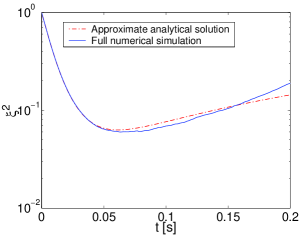
Figure 12: (Top) Spin squeezing with two-body losses in a bimodal Rb condensate as a function of time for symmetrically split condensates. Blue solid line: exact numerical simulation with 4000 realizations. Red dash-dotted line: analytical solution with constant loss rate approximation. (Bottom) Corresponding total number of particles and $\langle S_{z}\rangle$ as a function of time. Parameters: $\bar{N}_{a}=\bar{N}_{b}=10^{4}$, $\omega=2\pi\times 42.6$ Hz, $m$=87 a.m.u., $a_{aa}=100.44\,r_{B}$, $a_{bb}=95.47\,r_{B}$, $a_{ab}=88.28\,r_{B}$, $r_{B}$ is the Bohr radius, $\chi=5.367\times 10^{-3}$s^-1, $\tilde{\chi}=5.412\times 10^{-4}$s^-1, $v=13.758$ s^-1. Particle losses: $K_{2}^{(a)}=0$, $K_{2}^{(b)}=119\times 10^{-21}$m³s^-1.

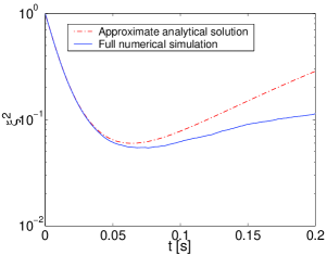
Figure 13: (Top) Spin squeezing with two-body losses in a bimodal Rb condensate as a function of time in breathe-together configuration. Blue solid line: exact numerical simulation with 4000 realizations. Red dash-dotted line: analytical solution with constant loss rate approximation. (Bottom) Corresponding total number of particles and $\langle S_{z}\rangle$ as a function of time. Parameters: $\bar{N}_{a}=7432$, $\bar{N}_{b}=12568$, $\chi=5.392\times 10^{-3}$s^-1, $\tilde{\chi}=1.386\times 10^{-3}$s^-1, $v=13.850$ s^-1. The other parameters are the same as in Fig.12.

The constant loss rate approximation neglects two effects: The decrease of the loss rate in time as less and less particles are in the system, and the change of the ratio $\langle N_{a}\rangle/\langle N_{b}\rangle$ as particles from the $b$ component are lost. In the case of Fig.12 where we consider initially $\langle N_{a}\rangle$=$\langle N_{b}\rangle$, which is the most favorable for squeezing, these two effects partially compensates: one tending to degrade and the other to improve the squeezing with respect to reality. In the case of Fig.13 instead, the two effects sum-up, both of them tending to degrade the squeezing with respect to reality. Note however that even for such large and completely non-symmetric losses, the constant loss rate approximation proves to be rather accurate up to the best squeezing time.

References

- (1) M. Kitagawa and M. Ueda, Phys. Rev. A 47, 5138 (1993).
- (2) J. Hald, J. L. Sørensen, C. Schori, and E. S. Polzik, Phys. Rev. Lett. 83, 1319 (1999); A. Kuzmich, L. Mandel, and N. P. Bigelow, Phys. Rev. Lett. 85, 1594 (2000).
- (3) D. J. Wineland, J. J. Bollinger, W. M. Itano, and D. J. Heinzen, Phys. Rev. A 50, 67 (1994).
- (4) D. Leibfried, M. D. Barrett, T. Schaetz, J. Britton, J. Chiaverini, W. M. Itano, J. D. Jost, C. Langer, D. J. Wineland Science 304, 1476 (2004).
- (5) G. Santarelli, Ph. Laurent, P. Lemonde, A. Clairon, A. G. Mann, S. Chang, and A. N. Luiten, and C. Salomon Phys. Rev. Lett. 82, 4619 (1999).
- (6) A. Sørensen, L. M. Duan, I. Cirac, and P. Zoller, Nature 409, 63 (2001).
- (7) B. Yurke, D. Stoler, Phys. Rev. Lett. 57, 13 (1986).
- (8) D. S. Hall, M. R. Matthews, J. R. Ensher, C. E. Wieman, and E. A. Cornell, Phys. Rev. Lett. 81, 1539 (1998).
- (9) A. Sinatra and Y. Castin, Eur. Phys. J. D 8, 319 (2000).
- (10) A. Sørensen, Phys. Rev. A 65, 043610 (2002).
- (11) S. Thanvanthri, and Z. Dutton, Phys. Rev. A 75, 023618 (2007).
- (12) Y. Li, Y. Castin, and A. Sinatra, Phys. Rev. Lett. 100, 210401 (2008).
- (13) P. Treutlein, P. Hommelhoff, T. Steinmetz, T. W. Häsch, and J. Reichel, Phys. Rev. Lett. 92, 203005 (2004).
- (14) M. Erhard, H. Schmaljohann, J. Kronjäger, K. Bongs, and K. Sengstock, Phys. Rev. A 69, 032705 (2004).
- (15) A. Widera, S. Trotzky, P. Cheinet, S. Fölling, F. Gerbier, I. Bloch, V. Gritsev, M. D. Lukin, and E. Demler, Phys. Rev. Lett. 100, 140401 (2008).
-
(16)
We can write the field operators as
,
and use the commutation
relations:
- (17) A. Sinatra and Y. Castin, Eur. Phys. J. D 4, 247 (1998)
- (18) Yu. Kagan, E. L. Surkov, and G. V. Shlyapnikov, Phys. Rev. A 54, R1753 (1996).
- (19) Y. Castin and R. Dum, Phys. Rev. Lett. 77, 5315 (1996).
- (20) S. Stringari, Phys. Rev. Lett. 77, 2360 (1996).
- (21) K. Mølmer, Y. Castin, J. Dalibard, J. Opt. Soc. Am. B 10, 524 (1993); H. J. Carmichael, An Open Systems Approach to Quantum Optics Springer, (1993).
- (22) A. Sinatra and Y. Castin, Eur. Phys. J. D 4, 247 (1998).
- (23) In the expression (65) of we replaced with consistently with the constant loss rate approximation.
- (24) K. M. Mertes, J. W. Merrill, R. Carretero-Gonzalez, D. J. Frantzeskakis, P. G. Kevrekidis, and D. S. Hall, Phys. Rev. Lett. 99 190402 (2007).
- (25) As we are pretty far from the Feshbach resonance, we assume for the crossed two-body loss rate the same value measured in Hall for the , states.
- (26) E. A. Burt, R. W. Ghrist, C. J. Myatt, M. J. Holland, E. A. Cornell, and C. E. Wieman, Phys. Rev. Lett. 79, 337 (1997).
- (27) D. M. Stamper-Kurn, M. R. Andrews, A. P. Chikkatur, S. Inouye, H.-J. Miesner, J. Stenger, and W. Ketterle, Phys. Rev. Lett. 80 2027 (1998).
- (28) P. Treutlein, T. W. Häsch, J. Reichel, A. Negretti, M. A. Cirone, and T. Calarco Phys. Rev. A 74 022312 (2006).
- (29) Uffe V. Poulsen and Klaus Mølmer, Phys. Rev. A 65 033613 (2002).
- (30) A. Couvert, T. Kawalec, G. Reinaudi, and D. Guéry-Odelin, arXiv: 0708.4197v1.
- (31) We checked that similar result can be obtained with different geometry where we prepare the condensate in a cigar shape and separate them along the longitudinal component.