Large-Sample Confidence Intervals for the Treatment Difference in a Two-Period Crossover Trial, Utilizing Prior Information

Department of Mathematics and Statistics, La Trobe University, Victoria 3086, Australia

Abstract

Consider a two-treatment, two-period crossover trial, with responses that are continuous random variables. We find a large-sample frequentist $1-\alpha$ confidence interval for the treatment difference that utilizes the uncertain prior information that there is no differential carryover effect.

Keywords: Differential carryover effect; Prior information; Two-period crossover trial.

^∗ Corresponding author. Address: Department of Mathematics and Statistics, La Trobe University, Victoria 3086, Australia; Tel.: +61-3-9479-2594; fax: +61-3-9479-2466. E-mail address: P.Kabaila@latrobe.edu.au.

1. Introduction

We consider a two-treatment two-period crossover trial, with responses that are continuous random variables. This design is very popular in a wide range of medical and other applications, see e.g. Jones and Kenward (1989) and Senn (2006). The purpose of this trial is to carry out inference about the difference $\theta$ in the effects of two treatments, labelled A and B. Subjects are randomly allocated to either group 1 or group 2. Subjects in group 1 receive treatment A in the first period and then receive treatment B in the second period. Subjects in group 2 receive treatment B in the first period and then receive treatment A in the second period. This design is efficient under the assumption that there is no differential carryover effect. It is not an appropriate design unless there is strong prior information that this assumption holds. However, a commonly occurring scenario is that it is not certain that this assumption holds. We consider this scenario. To deal with this uncertainty, it has been suggested (starting with Grizzle, 1965, 1974 and endorsed by Hills and Armitage, 1979) that a preliminary test of the null hypothesis that this assumption holds be carried out before proceeding with further inference. If this test leads to acceptance of this null hypothesis then further inference proceeds on the basis that it was known a priori that there is no differential carryover effect. If, on the other hand, this null hypothesis is rejected then further inference is based solely on data from the first period, since this is unaffected by any carryover effect. In a landmark paper, Freeman (1989) showed that the use of such a preliminary hypothesis test prior to the construction of a confidence interval with nominal coverage $1-\alpha$ leads to a confidence interval with minimum coverage probability far below $1-\alpha$. For simplicity, Freeman supposes that the subject variance and the error variance are known. In other words, Freeman presents a large-sample analysis. Freeman’s conclusion that the use of a preliminary test in this way ‘is too potentially misleading to be of practical use’ is now widely accepted (Senn, 2006). Freeman’s finding is consistent with the known deleterious effect of preliminary hypothesis tests on the coverage properties of subsequently-constructed confidence intervals in the context of a linear regression with independent and identically distributed zero-mean normal errors (see e.g. Kabaila, 2005; Kabaila and Leeb, 2006; Giri and Kabaila, 2008; Kabaila and Giri, 2008).

A Bayesian analysis that incorporates prior information about the differential carryover effect is provided by Grieve (1985, 1986). However, there is currently no valid frequentist confidence interval for the difference $\theta$ of the two treatment effects that utilizes the uncertain prior information that there is no differential carryover effect. Similarly to Hodges and Lehmann (1952), Bickel (1983, 1984), Kabaila (1998), Kabaila and Giri (2007ab), Farchione and Kabaila (2008) and Kabaila and Tuck (2008), our aim is to utilize the uncertain prior information in the frequentist inference of interest, whilst providing a safeguard in case this prior information happens to be incorrect. We follow Freeman (1989) and assume that the between-subject variance and the error variance are known. As already noted, this corresponds to a large-sample analysis. The usual $1-\alpha$ confidence interval for $\theta$ based solely on data from the first period is unaffected by any differential carryover effect. We use this interval as the standard against which other $1-\alpha$ confidence intervals will be assessed. We therefore call this confidence interval the ‘standard $1-\alpha$ confidence interval’. We assess a $1-\alpha$ confidence interval for $\theta$ using the ratio

$$\frac{\text{expected length of this confidence interval}}{\text{length of the standard $1-\alpha$ confidence interval}.}$$

We call this ratio the scaled expected length of this confidence interval. We find a new $1-\alpha$ confidence interval that utilizes the uncertain prior information that the differential carryover effect is zero, in the following sense. This new interval has scaled expected length that (a) is substantially less than 1 when the prior information that there is no differential carryover effect holds and (b) has a maximum value that is not too large. Also, this confidence interval coincides with the standard $1-\alpha$ confidence interval when the data strongly contradicts the prior information that there is no differential carryover effect. Additionally, this confidence interval has the attractive feature that it has endpoints that are continuous functions of the data.

The properties of the new large-sample confidence interval, described in Section 2, are illustrated in Section 3 by a detailed analysis of the case that the between-subject variance and the error variance are equal and $1-\alpha=0.95$. In Section 2, we define the parameter $\gamma$ to be the differential carryover divided by the standard deviation of the least squares estimator of the differential carryover. As proved in Section 2, the coverage probability of the new confidence interval for $\theta$ is an even function of $\gamma$. The top panel of Figure 2 is a plot of the coverage probability of the new 0.95 confidence interval for $\theta$ as a function of $\gamma$. This plot shows that the new 0.95 confidence interval for $\theta$ has coverage probability 0.95 throughout the parameter space. As proved in Section 2, the scaled expected length of the new confidence interval for $\theta$ is an even function of $\gamma$. The bottom panel of Figure 2 is a plot of the square of the scaled expected length of the new 0.95 confidence interval for $\theta$ as a function of $\gamma$. When the prior information is correct (i.e. $\gamma=0$), we gain since the square of the scaled expected length is substantially smaller than 1. The maximum value of the square of the scaled expected length is not too large. The new 0.95 confidence interval for $\theta$ coincides with the standard $1-\alpha$ confidence interval when the data strongly contradicts the prior information. This is reflected in Figure 2 by the fact that the square of the scaled expected length approaches 1 as $\gamma\rightarrow\infty$.

In Section 4, we compare the two-period crossover trial with a completely randomized design with the same number of measurements of response, using a large sample analysis. We assume that the new 0.95 confidence interval is used to summarise the data from the two-period crossover trial. We show that the uncertainty in the prior information that there is no differential carryover effect has the following consequence. Subject to a reasonable upper bound on how badly the new 0.95 confidence interval can perform relative to the usual 0.95 confidence interval for $\theta$ based on data from the completely randomized design, the completely randomized design is better than the two-period crossover trial for all (subject variance)/(error variance) $\in(0,11.6263]$. In Section 5 we describe the implications for finite samples of the results described in Sections 3 and 4.

2. New large-sample confidence interval utilizing prior information about the differential carryover effect

We assume the model for the two-treatment two-period crossover trial put forward by Grizzle (1965), as described by Grieve (1987). Let $n_{1}$ and $n_{2}$ denote the number of subjects in groups 1 and 2 respectively. Also let $Y_{ijk}$ denote the response of the $j$th subject in the $i$th group and the $k$th period ($i=1,2$; $j=1,\ldots,n_{i}$; $k=1,2$). The model is

$$Y_{ijk}=\mu+\xi_{ij}+\pi_{k}+\phi_{\ell}+\lambda_{\ell}+\varepsilon_{ijk}$$

where $\mu$ is the overall population mean, $\xi_{ij}$ is the effect of the $j$th patient in the $i$th group, $\pi_{k}$ is the effect of the $k$th period, $\phi_{\ell}$ is the effect of the $\ell$th treatment, $\lambda_{\ell}$ is the residual effect of the $\ell$th treatment and $\varepsilon_{ijk}$ is the random error. We assume that the $\xi_{ij}$ and $\varepsilon_{ijk}$ are independent and that the $\xi_{ij}$ are identically $N(0,\sigma_{s}^{2})$ distributed and the $\varepsilon_{ijk}$ are identically $N(0,\sigma_{\varepsilon}^{2})$ distributed, where $\sigma_{s}^{2}>0$ and $\sigma_{\varepsilon}^{2}>0$. Let $m=(1/n_{1})+(1/n_{2})$, $\sigma^{2}=\sigma_{\varepsilon}^{2}+\sigma_{s}^{2}$ and $\rho=\sigma_{s}^{2}/(\sigma_{\varepsilon}^{2}+\sigma_{s}^{2})$. The parameter of interest is $\theta=\phi_{1}-\phi_{2}$. The parameter describing the differential carryover effect is $\psi=(\lambda_{1}-\lambda_{2})/2$. We suppose that we have uncertain prior information that $\psi=0$.

We use the notation $\bar{Y}_{i\boldsymbol{\cdot}\,k}=(1/n_{i})\sum_{j=1}^{n_{1}}Y_{ijk}$ ($i=1,2$). Our statistical analysis will be described entirely in terms of the following random variables: $A=\big{(}\bar{Y}_{1\boldsymbol{\cdot}1}-\bar{Y}_{1\boldsymbol{\cdot}2}-\bar{Y}_{2\boldsymbol{\cdot}1}+\bar{Y}_{2\boldsymbol{\cdot}2}\big{)}/2$, $\hat{\Psi}=\big{(}\bar{Y}_{1\boldsymbol{\cdot}1}+\bar{Y}_{1\boldsymbol{\cdot}2}-\bar{Y}_{2\boldsymbol{\cdot}1}-\bar{Y}_{2\boldsymbol{\cdot}2}\big{)}/2$,

$$V =\frac{1}{2}\left(\sum_{j=1}^{n_{1}}\left((Y_{1j1}-\bar{Y}_{1\boldsymbol{\cdot}1})-(Y_{1j2}-\bar{Y}_{1\boldsymbol{\cdot}2})\right)^{2}+\sum_{j=1}^{n_{2}}\left((Y_{2j1}-\bar{Y}_{2\boldsymbol{\cdot}1})-(Y_{2j2}-\bar{Y}_{2\boldsymbol{\cdot}2})\right)^{2}\right),$$

$$W =\frac{1}{2}\left(\sum_{j=1}^{n_{1}}\left((Y_{1j1}-\bar{Y}_{1\boldsymbol{\cdot}1})+(Y_{1j2}-\bar{Y}_{1\boldsymbol{\cdot}2})\right)^{2}+\sum_{j=1}^{n_{2}}\left((Y_{2j1}-\bar{Y}_{2\boldsymbol{\cdot}1})+(Y_{2j2}-\bar{Y}_{2\boldsymbol{\cdot}2})\right)^{2}\right).$$

These random variables are independent and they have the following distributions: $A\sim N\big{(}\theta-\psi,m\sigma_{\varepsilon}^{2}/2\big{)}$, $\hat{\Psi}\sim N\big{(}\psi,m(\sigma_{\varepsilon}^{2}+2\sigma_{s}^{2})/2\big{)}$, $V/\sigma_{\varepsilon}^{2}\sim\chi_{n_{1}+n_{2}-2}^{2}$ and $W/(\sigma_{\varepsilon}^{2}+2\sigma_{s}^{2})\sim\chi_{n_{1}+n_{2}-2}^{2}$. Define $\hat{\Theta}=A+\hat{\Psi}=\bar{Y}_{1\boldsymbol{\cdot}1}-\bar{Y}_{2\boldsymbol{\cdot}1}$. This estimator of $\theta$ is based solely on the data from period 1. Consequently, it is not influenced by any carryover effects. Note that

$$\left[\begin{matrix}\hat{\Theta}\\ \hat{\Psi}\end{matrix}\right]\sim N\left(\left[\begin{matrix}\theta\\ \psi\end{matrix}\right],\sigma^{2}\left[\begin{matrix}m\quad\quad m\tilde{\rho}^{2}\\ m\tilde{\rho}^{2}\quad m\tilde{\rho}^{2}\end{matrix}\right]\right).$$ (1)

where $\tilde{\rho}$ denotes the correlation between $\hat{\Theta}$ and $\hat{\Psi}$ and is equal to $\sqrt{(1+\rho)/2}$.

We follow Freeman (1989) and assume that the subject variance $\sigma_{s}^{2}$ and the error variance $\sigma_{\varepsilon}^{2}$ are known. This implies that the parameters $\sigma^{2}$ and $\tilde{\rho}$ are known. Using the random variables $V$ and $W$ in the obvious way, $\sigma_{s}^{2}$ and $\sigma_{\varepsilon}^{2}$ can be estimated consistently as $n_{1}+n_{2}\rightarrow\infty$. In other words, we are using a large-sample analysis.

We use the notation $[a\pm b]$ for the interval $[a-b,a+b]$ ($b>0$). Define $c_{\alpha}=\Phi^{-1}(1-\frac{\alpha}{2})$, where $\Phi$ denotes the $N(0,1)$ cumulative distribution function. The usual $1-\alpha$ confidence interval for $\theta$, based solely on data from the first period, is $I=\big{[}\hat{\Theta}\pm c_{\alpha}\sqrt{m}\sigma\big{]}$. Define the following confidence interval for $\theta$:

$$J(b,s)=\bigg{[}\hat{\Theta}-\sqrt{m}\sigma\,b\bigg{(}\frac{\hat{\Psi}}{\sigma\sqrt{m}\tilde{\rho}}\bigg{)}\,\pm\,\sqrt{m}\sigma\,s\bigg{(}\frac{|\hat{\Psi}|}{\sigma\sqrt{m}\tilde{\rho}}\bigg{)}\bigg{]},$$

where the functions $b$ and $s$ are required to satisfy the following restriction.

Restriction 1  $b:\mathbb{R}\rightarrow\mathbb{R}$ is an odd function and $s:[0,\infty)\rightarrow[0,\infty)$.

Invariance arguments, of the type used by Farchione and Kabaila (2008), may be used to motivate this restriction. For the sake of brevity, these arguments are omitted. We also require the functions $b$ and $s$ to satisfy the following restriction.

Restriction 2  $b$ and $s$ are continuous functions.

This implies that the endpoints of the confidence interval $J(b,s)$ are continuous functions of the data. Finally, we require the confidence interval $J(b,s)$ to coincide with the standard $1-\alpha$ confidence interval $I$ when the data strongly contradict the prior information. The statistic $|\hat{\Psi}|/(\sigma\sqrt{m}\tilde{\rho})$ provides some indication of how far away $\psi/(\sigma\sqrt{m}\tilde{\rho})$ is from 0. We therefore require that the functions $b$ and $s$ satisfy the following restriction.

Restriction 3  $b(x)=0$ for all $|x|\geq d$ and $s(x)=c_{\alpha}$ for all $x>d$, where $d$ is a (sufficiently large) specified positive number.

Define $\gamma=\psi/(\sigma\sqrt{m}\tilde{\rho})$, $G=(\hat{\Theta}-\theta)/(\sigma\sqrt{m})$ and $H=\hat{\Psi}/(\sigma\sqrt{m}\tilde{\rho})$. It follows from (1) that

$$\left[\begin{matrix}G\\ H\end{matrix}\right]\sim N\left(\left[\begin{matrix}0\\ \gamma\end{matrix}\right],\left[\begin{matrix}1\quad\tilde{\rho}\\ \tilde{\rho}\quad 1\end{matrix}\right]\right).$$ (2)

It is straightforward to show that the coverage probability $P\big{(}\theta\in J(b,s)\big{)}$ is equal to $P\big{(}\ell(H)\leq G\leq u(H)\big{)}$ where $\ell(h)=b(h)-s(|h|)$ and $u(h)=b(h)+s(|h|)$. For given $b$, $s$ and $\tilde{\rho}$, this coverage probability is a function of $\gamma$. We denote this coverage probability by $c(\gamma;b,s,\tilde{\rho})$.

Part of our evaluation of the confidence interval $J(b,s)$ consists of comparing it with the standard $1-\alpha$ confidence interval $I$ using the criterion

$$\frac{\text{expected length of $J(b,s)$}}{\text{length of $I$}}.$$ (3)

We call this the scaled expected length of $J(b,s)$. This is equal to $E(s(|H|))/c_{\alpha}$. This is a function of $\gamma$ for given $s$. We denote this function by $e(\gamma;s)$. Clearly, for given $s$, $e(\gamma;s)$ is an even function of $\gamma$.

Our aim is to find functions $b$ and $s$ that satisfy Restrictions 1–3 and such that (a) the minimum of $c(\gamma;b,s,\tilde{\rho})$ over $\gamma$ is $1-\alpha$ and (b)

$$\int_{-\infty}^{\infty}(e(\gamma;s)-1)\,d\nu(\gamma)$$ (4)

is minimized, where the weight function $\nu$ has been chosen to be

$$\nu(x)=\omega x+{\cal H}(x)\ \text{ for all }\ x\in\mathbb{R},$$

where $\omega$ is a specified nonnegative number and ${\cal H}$ is the unit step function defined by ${\cal H}(x)=1$ for $x\geq 0$ and ${\cal H}(x)=0$ for $x<0$. The larger the value of $\omega$, the smaller the relative weight given to minimizing $e(\gamma;s)$ for $\gamma=0$, as opposed to minimizing $e(\gamma;s)$ for other values of $\gamma$.

The following theorem (cf. Kabaila and Giri, 2007a) provides computationally convenient expressions for the coverage probability and scaled expected length of $J(b,s)$.

Theorem 2.1

(a) Define the functions $k^{{\dagger}}(h,\gamma,\tilde{\rho})=\Lambda\left(-c_{\alpha},c_{\alpha};\tilde{\rho}(h-\gamma),1-\tilde{\rho}^{2}\right)$ and $k(h,\gamma,\tilde{\rho})=\Lambda\left(\ell(h),u(h);\tilde{\rho}(h-\gamma),1-\tilde{\rho}^{2}\right)$, where $\Lambda(x,y;\mu,v)=P(x\leq Z\leq y)$ for $Z\sim N(\mu,v)$. The coverage probability $P\big{(}\theta\in J(b,s)\big{)}$ is equal to

$$(1-\alpha)+\int_{-d}^{d}\big{(}k(h,\gamma,\tilde{\rho})-k^{{\dagger}}(h,\gamma,\tilde{\rho})\big{)}\,\phi(h-\gamma)\,dh,$$ (5)

where $\phi$ denotes the $N(0,1)$ probability density function. For given $b$, $s$ and $\tilde{\rho}$, $c(\gamma;b,s,\tilde{\rho})$ is an even function of $\gamma$.

(b) The scaled expected length of $J(b,s)$ is

$$e(\gamma;s)=1+\frac{1}{c_{\alpha}}\int^{d}_{-d}\left(s(|h|)-c_{\alpha}\right)\phi(h-\gamma)\,dh.$$ (6)

Substituting (6) into (4) we obtain that (4) is equal to

$$\frac{1}{c_{\alpha}}\int_{-\infty}^{\infty}\int^{d}_{-d}\left(s(|h|)-c_{\alpha}\right)\phi(h-\gamma)\,dh\,d\nu(\gamma)=\frac{2}{c_{\alpha}}\int^{d}_{0}\left(s(h)-c_{\alpha}\right)(\omega+\phi(h))\,dh.$$ (7)

For computational feasibility, we specify the following parametric forms for the functions $b$ and $s$. We require $b$ to be a continuous function and so it is necessary that $b(0)=0$. Suppose that $x_{1},\ldots,x_{q}$ satisfy $0=x_{1}<x_{2}<\cdots<x_{q}=d$. Obviously, $b(x_{1})=0$, $b(x_{q})=0$ and $s(x_{q})=c_{\alpha}$. The function $b$ is fully specified by the vector $\big{(}b(x_{2}),\ldots,b(x_{q-1})\big{)}$ as follows. Because $b$ is assumed to be an odd function, we know that $b(-x_{i})=-b(x_{i})$ for $i=2,\ldots,q$. We specify the value of $b(x)$ for any $x\in[-d,d]$ by cubic spline interpolation for these given function values, subject to the constraint that $b^{\prime}(-d)=0$ and $b^{\prime}(d)=0$. We fully specify the function $s$ by the vector $\big{(}s(x_{1}),\ldots,s(x_{q-1})\big{)}$ as follows. The value of $s(x)$ for any $x\in[0,d]$ is specified by cubic spline interpolation for these given function values (without any endpoint conditions on the first derivative of $s$). We call $x_{1},x_{2},\ldots x_{q}$ the knots.

To conclude this section, the new $1-\alpha$ confidence interval for $\theta$ that utilizes the prior information that $\psi=0$ is obtained as follows. For a judiciously-chosen set of values of $d$, $\omega$ and knots $x_{i}$, we carry out the following computational procedure.

Computational Procedure  Compute the functions $b$ and $s$, satisfying Restrictions 1–3 and taking the parametric forms described above, such that (a) the minimum over $\gamma\geq 0$ of (5) is $1-\alpha$ and (b) the criterion (7) is minimized. Plot $e^{2}(\gamma;s)$, the square of the scaled expected length, as a function of $\gamma\geq 0$.

Based on these plots and the strength of our prior information that $\psi=0$, we choose appropriate values of $d$, $\omega$ and knots $x_{i}$. The confidence interval corresponding to this choice is the new $1-\alpha$ confidence interval for $\theta$. For given $\omega$, the functions $b$ and $s$ can be chosen to be functions of $\tilde{\rho}$, since $\tilde{\rho}$ is assumed to be known. All the computations for the present paper were performed with programs written in MATLAB, using the Optimization and Statistics toolboxes.

3. Illustration of the properties of the new confidence interval

The parameter $\tilde{\rho}$ lies in the interval $\big{(}1/\sqrt{2},\,1\big{)}$. To illustrate the properties of the new $1-\alpha$ confidence interval for $\theta$, consider the case that $\sigma_{s}^{2}/\sigma_{\varepsilon}^{2}=1$, so that $\tilde{\rho}=\sqrt{3}/2$. Suppose that $1-\alpha=0.95$. We have followed the Computational Procedure, described in the previous section, with $d=6$, $\omega=0.2$ and evenly-spaced knots at $0,6/8,\ldots,6$. The resulting functions $b$ and $s$, which specify the new 0.95 confidence interval for $\theta$, are plotted in Figure 1. The performance of this confidence intervals is shown in Figure 2. When the prior information is correct (i.e. $\gamma=0$), we gain since $e^{2}(0;s)=0.8527$. The maximum value of $e^{2}(\gamma;s)$ is 1.1239. This confidence interval coincides with the standard $1-\alpha$ confidence interval for $\theta$ when the data strongly contradicts the prior information, so that $e^{2}(\gamma;s)$ approaches 1 as $\gamma\rightarrow\infty$.

The value of $\omega=0.2$ was obtained from the following search. Consider $\omega=0.05$, 0.2 , 0.5 and 1. The Computational Procedure was applied for each of these values. As expected from the form of the weight function, for each of these values of $\omega$, $e^{2}(\gamma;s)$ is minimized at $\gamma=0$. For a given value of $\lambda$, define the ‘expected gain’ to be $\big{(}1-e^{2}(0;s)\big{)}$ and the ‘maximum potential loss’ to be $\big{(}\max_{\gamma}e^{2}(\gamma;s)-1\big{)}$. As shown in Table 1, as $\omega$ increases (a) the expected gain decreases and (b) the ratio (expected gain)/(maximum potential loss) increases. By choosing $\omega=0.2$ we have both a reasonably large expected gain and a reasonably large value of the ratio (expected gain)/(maximum potential loss).

$\omega$	0.05	0.2	0.5	1
expected gain	0.2173	0.1473	0.0904	0.0542
maximum potential loss	0.2982	0.1239	0.0595	0.0324
(expected gain)/(maximum potential loss)	0.7288	1.1892	1.5206	1.6704

Table 1: Performance of the 0.95 confidence interval for $d=6$ and evenly-spaced knots at $0,6/8,\ldots,6$, when we vary over $\omega\in\{0.05,0.2,0.5,1\}$.

4. Comparison of the two-period crossover trial with a completely
randomized design with the same number of measurements of response

For the two-period crossover trial, the total number of measurements of response is $2M$, where $M=n_{1}+n_{2}$. Following Brown (1980), we compare this design with a completely randomized design with the same total number of measurements of the response. For the completely randomized design, we have $M$ randomly-chosen subjects given treatment A and $M$ randomly-chosen subjects given treatment B. Let $Y_{1}^{A},\ldots,Y_{M}^{A}$ denote the responses for the $M$ subjects given treatment A and let $Y_{1}^{B},\ldots,Y_{M}^{B}$ denote the responses for the $M$ subjects given treatment B. A model for these responses that is consistent with the model used for the two-period crossover trial is the following. Suppose that $Y_{1}^{A},\ldots,Y_{M}^{A},Y_{1}^{B},\ldots,Y_{M}^{B}$ are independent random variables, with $Y_{1}^{A},\ldots,Y_{M}^{A}$ identically $N(\phi_{1},\sigma^{2})$ distributed and $Y_{1}^{B},\ldots,Y_{M}^{B}$ identically $N(\phi_{2},\sigma^{2})$ distributed. The usual estimator of $\theta=\phi_{1}-\phi_{2}$ is $\widetilde{\Theta}=\big{(}(Y_{1}^{A}+\cdots+Y_{M}^{A})-(Y_{1}^{B}+\cdots+Y_{M}^{B})\big{)}/M$. Obviously, $\widetilde{\Theta}\sim N(\theta,2\sigma^{2}/M)$.

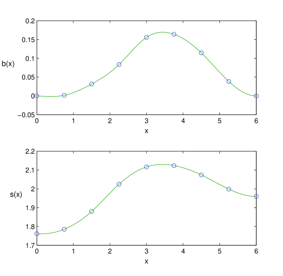
Figure 1: Plots of the functions $b$ and $s$ for $\sigma_{s}^{2}/\sigma_{\varepsilon}^{2}=1$ and $1-\alpha=0.95$. These functions were obtained using $d=6$, $\omega=0.2$ and evenly-spaced knots $x_{i}$ at $0,6/8,\ldots,6$.

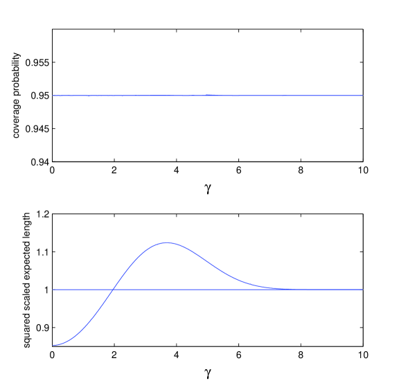
Figure 2: Plots of the coverage probability and $e^{2}(\gamma;s)$, the squared scaled expected length, (as functions of $\gamma=\psi/\sqrt{\text{var}(\hat{\Psi})}$) of the new 0.95 confidence interval for $\theta$ when $\sigma_{s}^{2}/\sigma_{\varepsilon}^{2}=1$. These functions were obtained using $d=6$, $\omega=0.2$ and evenly-spaced knots $x_{i}$ at $0,6/8,\ldots,6$.

Now, following Brown (1980), consider the case that there is no differential carryover effect i.e. that $\psi=0$. In this case, $\theta$ is estimated by $A\sim N(\theta,m\sigma_{\varepsilon}^{2}/2)$. Thus

$$\frac{\text{var}(A)}{\text{var}(\widetilde{\Theta})}=\frac{n_{1}+n_{2}}{4}\left(\frac{1}{n_{1}}+\frac{1}{n_{2}}\right)\frac{1}{1+(\sigma_{s}^{2}/\sigma_{\varepsilon}^{2})}.$$

As this expression shows, the efficiency of the two-period crossover trial, relative to the completely randomized design, is an increasing function of $\sigma_{s}^{2}/\sigma_{\varepsilon}^{2}$. For the case $n_{1}=n_{2}=n$, the two-period crossover trial is more efficient than the completely randomized design for all $\sigma_{s}^{2}/\sigma_{\varepsilon}^{2}>0$. In other words, if we are absolutely certain that there is no differential carryover effect then we should always use the two-period crossover trial, as opposed to the completely randomized design.

However, as noted in the introduction, it is commonly the case that it is not certain that there is no differential carryover effect. We ask the following question. What is the efficiency of the two-period crossover trial relative to the completely randomized design in this case? We consider this question in the context that $\sigma_{s}^{2}$ and $\sigma_{\varepsilon}^{2}$ are known. In other words, we consider this question in the context of large samples. We also assume that the new $1-\alpha$ confidence interval described in Section 2 is used to summarise the data from the two-period crossover trial. For simplicity suppose that $n_{1}=n_{2}=n$. Based on data from a completely randomized design, that usual $1-\alpha$ confidence interval for $\theta$ is $K=\big{[}\widetilde{\Theta}\pm c_{\alpha}\sigma/\sqrt{n}\big{]}$. In earlier sections, we have assessed the new $1-\alpha$ confidence interval using the scaled expected length criterion (3), denoted by $e(\gamma;s)$. To compare the two-period crossover trial with a completely randomized design with the same total number of measurements, we now use the criterion

$$r(\gamma;s)=\frac{\text{expected length of $J(b,s)$}}{\text{length of $K$}}.$$

Note that $r(\gamma;s)=\sqrt{2}\,e(\gamma;s)$, so that $r^{2}(\gamma;s)=2\,e^{2}(\gamma;s)$. For a given value of $\tilde{\rho}\in(1/\sqrt{2},1)$, let us restrict attention to the class ${\cal C}(\tilde{\rho},1-\alpha)$ of new $1-\alpha$ confidence intervals that satisfy the constraint $\max_{\gamma}e^{2}(\gamma;s)\leq 1.25$, so that

$$\max_{\gamma}r^{2}(\gamma;s)\leq 1.5.$$ (8)

This condition puts an upper bound on how badly the new $1-\alpha$ confidence interval can perform relative to the confidence interval $K$ based on data from the completely randomized design. Consider the particular case that $1-\alpha=0.95$. For each $\tilde{\rho}\in(1/\sqrt{2},0.98]$, i.e. for each $\sigma_{s}^{2}/\sigma_{\varepsilon}^{2}\in(0,11.6263]$, we find computationally that $\min_{\gamma}r^{2}(\gamma;s)>1$ for every new $1-\alpha$ confidence interval belonging to ${\cal C}(\tilde{\rho},0.95)$. In other words, if we impose the reasonable constraint (8) then, for $1-\alpha=0.95$ and large samples, the completely randomized design is better than the two-period crossover trial for each $\sigma_{s}^{2}/\sigma_{\varepsilon}^{2}\in(0,11.6263]$. This is a complete contrast to the case that we are absolutely certain that there is no differential carryover effect.

5. Implications for finite samples

By replacing the parameters $\sigma$ and $\tilde{\rho}$ by their obvious estimators (based on the statistics $V$ and $W$) in the new large-sample $1-\alpha$ confidence interval described in Section 2, we obtain a new finite-sample confidence interval for $\theta$. This new finite-sample confidence interval will have coverage and scaled expected length properties that will approach the corresponding properties for the new large-sample $1-\alpha$ confidence interval as $n_{1}+n_{2}\rightarrow\infty$. This suggests that it will be possible to design confidence intervals for $\theta$ that utilize the uncertain prior information that there is no differential carryover effect for small and medium, as well as large sample sizes. This also suggests that the result found in Section 4 will also be reflected in small and medium, as well as large samples sizes. We expect that subject to a reasonable upper bound on how badly any new finite-sample 0.95 confidence interval can perform relative to the usual 0.95 confidence interval for $\theta$ based on data from the completely randomized design, the completely randomized design is better than the two-period crossover trial for a very wide range of values of (subject variance)/(error variance).

Appendix. Proof of Theorem 2.1

In this appendix we prove Theorem 2.1.

Proof of part (a).  It follows from (2) that the probability density function of $H$, evaluated at $h$, is $\phi(h-\gamma)$. Thus

$$c(\gamma;b,s,\tilde{\rho})=\int_{-\infty}^{\infty}\int_{\ell(h)}^{u(h)}f_{G|H}(g|h)\,dg\,\phi(h-\gamma)\,dh$$ (A.1)

where $f_{G|H}(g|h)$ denotes the probability density function of $G$ conditional on $H=h$, evaluated at $g$. The probability distribution of $G$ conditional on $H=h$ is $N\big{(}\tilde{\rho}(h-\gamma),1-\tilde{\rho}^{2}\big{)}$. Thus the right hand side of (A.1) is equal to

$$\int_{-\infty}^{\infty}k(h,\gamma,\tilde{\rho})\,\phi(h-\gamma)\,dh$$ (A.2)

The standard $1-\alpha$ confidence interval $I$ has coverage probability $1-\alpha$. Hence

$$1-\alpha=\int_{-\infty}^{\infty}k^{{\dagger}}(h,\gamma,\tilde{\rho})\,\phi(h-\gamma)\,dh.$$ (A.3)

The result follows from subtracting (A.3) from (A.2) and noting that $b(x)=0$ for all $|x|\geq d$ and $s(x)=c_{\alpha}$ for all $x\geq d$. By a consideration of the distribution of $(-G,-H)$, it may be shown that $c(\gamma;b,s,\tilde{\rho})$ is an even function of $\gamma$, for given $b$, $s$ and $\tilde{\rho}$.

Proof of part (b). The result is an immediate consequence of the fact that $b(x)=0$ for all $|x|\geq d$ and $s(x)=c_{\alpha}$ for all $x\geq d$.

References

Bickel, P.J., 1983. Minimax estimation of the mean of a normal distribution subject to doing well at a point. In: Rizvi, M.H., Rustagi, J.S., Siegmund, D., (Eds), Recent Advances in Statistics, Academic Press, New York, 511–528.

Bickel, P.J., 1984. Parametric robustness: small biases can be worthwhile. Annals of Statistics 12, 864–879.

Brown, B.W., 1980. The crossover experiment in clinical trials. Biometrics 36, 69–79.

Farchione, D., Kabaila, P., 2008. Confidence intervals for the normal mean utilizing prior information. Statistics & Probability Letters 78, 1094–1100.

Freeman, P.R., 1989. The performance of the two-stage analysis of two-treatment, two-period crossover trials. Statistics in Medicine 8, 1421–1432.

Giri, K., Kabaila, P., 2008. The coverage probability of confidence intervals in $2^{r}$ factorial experiments after preliminary hypothesis testing. Australian & New Zealand Journal of Statistics 50, 69–79.

Grieve, A.P., 1985. A Bayesian analysis of the two-period crossover design for clinical trials. Biometrics 41, 979–990.

Grieve, A.P., 1986. Corrigenda to Grieve (1985). Biometrics 42, 459.

Grieve, A.P., 1987. A note on the analysis of a two-period crossover design when the period-treatment interaction is significant. Biometrical Journal 7, 771–776.

Grizzle, J.E., 1965. The two-period change-over design and its use in clinical trials. Biometrics 21, 467–480.

Grizzle, J.E., 1974. Corrigenda to Grizzle (1965). Biometrics 30, 727.

Hills, M., Armitage, P., 1979. The two-period cross-over clinical trial. British Journal of Pharmacology 8, 7–20.

Hodges, J.L., Lehmann, E.L., 1952. The use of previous experience in reaching statistical decisions. Annals of Mathematical Statistics 23, 396–407.

Jones, B., Kenward, M.G., 1989. Design and Analysis of Cross-Over Trials. Chapman & Hall, London.

Kabaila, P., 1998. Valid confidence intervals in regression after variable selection. Econometric Theory 14, 463–482.

Kabaila, P., 2005. On the coverage probability of confidence intervals in regression after variable selection. Australian & New Zealand Journal of Statistics 47, 549–562.

Kabaila, P., Giri, K., 2007a. Large sample confidence intervals in regression utilizing prior information. La Trobe University, Department of Mathematics and Statistics, Technical Report No. 2007–1, Jan 2007.

Kabaila, P., Giri, K., 2007b. Confidence intervals in regression utilizing prior information. arXiv:0711.3236. Submitted for publication.

Kabaila, P., Giri, K., 2008. Upper bounds on the minimum coverage probability of confidence intervals in regression after variable selection. To appear in Australian & New Zealand Journal of Statistics.

Kabaila, P., Leeb, H., 2006. On the large-sample minimal coverage probability of confidence intervals after model selection. Journal of the American Statistical Association 101, 619–629.

Kabaila, P., Tuck, J., 2008. Confidence intervals utilizing prior information in the Behrens-Fisher problem. To appear in Australian & New Zealand Journal of Statistics.

Pratt, J.W., 1961. Length of confidence intervals. Journal of the American Statistical Association 56, 549–657.

Senn, S., 2006. Cross-over trials in Statistics in Medicine: the first ‘25’ years. Statistics in Medicine 25, 3430–3442.