Is the Gini coefficient a stable measure of galaxy structure?

Abstract

The Gini coefficient, a non-parametric measure of galaxy morphology, has recently taken up an important role in the automated identification of galaxy mergers. I present a critical assessment of its stability, based on a comparison of HST/ACS imaging data from the GOODS and UDF surveys. Below a certain signal-to-noise level, the Gini coefficient depends strongly on the signal-to-noise ratio, and thus becomes useless for distinguishing different galaxy morphologies. Moreover, at all signal-to-noise levels the Gini coefficient shows a strong dependence on the choice of aperture within which it is measured. Consequently, quantitative selection criteria involving the Gini coefficient, such as a selection of merger candidates, cannot always be straightforwardly applied to different datasets. I discuss whether these effects could have affected previous studies that were based on the Gini coefficient, and establish signal-to-noise limits above which measured Gini values can be considered reliable.

1. Introduction and Motivation

The ever increasing amount of galaxies probed by imaging surveys such as the Sloan Digital Sky Survey (SDSS, Stoughton et al., 2002), the Great Observatories Origins Deep Survey (GOODS, Giavalisco et al., 2004), or the Hubble Space Telescope (HST) Ultra Deep Field (UDF, Beckwith et al., 2006) triggered the need for automated galaxy classification methods. Ideally, these should not only be faster in classifying thousands of galaxies than any visual examination, but should be more robust and less subjective than the latter.

An important aspect is the evolution of galaxy structure over cosmic time: deep HST surveys such as GOODS or UDF reveal a huge amount of peculiar or irregular galaxies (see, e.g., Cowie et al., 1995b; Elmegreen et al., 2004a; Conselice et al., 2008) that do not fit into the standard Hubble scheme, nor into the class of irregular galaxies as defined for the local Universe. This is owed to the fact that more distant galaxies are seen in a significantly younger stage, in which starburst events and mergers occur at a larger rate (e.g. Cowie et al., 1995a; Madau et al., 1998; Bell et al., 2006a). Moreover, at higher redshifts, bluer rest-frame wavelengths are probed, giving emphasis to the distribution of the young stellar component. Although trust in visual classification remains for both low-redshift (e.g. Schawinski et al., 2007) and high-redshift datasets (e.g. Ferreras et al., 2005), the hope was that new structural classification schemes would also be suitable to describe the various kinds of peculiar galaxies in an appropriate way (Abraham et al., 1994, 1996b), and to separate them from the more familiar galaxy classes.

“Non-parametric” structural measures that have been developed in this context are the concentration index ($C$, Abraham et al., 1994; Bershady et al., 2000; Trujillo et al., 2001; Graham et al., 2001; Conselice, 2003), the asymmetry index ($A$, Abraham et al., 1996a; Conselice, 1997; Kornreich et al., 1998; Conselice et al., 2000), and the clumpiness index ($S$, Conselice, 2003). These three are known as the CAS parameters (Conselice, 2003). Two further parameters that are frequently used are the Gini coefficient (Gini, 1912; Abraham et al., 2003; Lotz et al., 2004) and the $M_{20}$ parameter (Lotz et al., 2004). Gini describes the distribution of flux values among the pixels of an object’s image, while $M_{20}$ quantifies the distribution of the brightest 20% of pixels. As opposed to the CAS parameters, neither Gini nor $M_{20}$ require the center of a galaxy to be defined, and thus do not need to assume that a well-defined visible center exists at all. All these parameters are commonly dubbed “non-parametric”, since they do not rely on certain model parameter fits, such as the Sérsic index (Sérsic, 1963) in models of radial surface brightness profiles. A more appropriate term might therefore be “model-independent”.

One particular application of these model-independent measures was the identification of galaxy mergers. Studying their abundance and properties is crucial to understand the origin of the most massive galaxies in the Universe today (e.g. Bell et al., 2006b), of which many must have formed within the last gigayears (Bell et al., 2004; Ferreras et al., 2005). Conselice et al. (2003a) selected major galaxy mergers as objects with a rest-frame $B$-band asymmetry index of $A\geq 0.35$, and used it to derive merger fractions and subsequently galaxy merger rates out to a redshift of $z\approx 3$. By applying this structural selection to submillimeter-detected galaxies, Conselice et al. (2003b) concluded that many of these are undergoing a major merger. Lotz et al. (2006) studied the fraction of major mergers and minor merger candidates among high-redshift star-forming galaxies, using a classification based on Gini, $M_{20}$, and concentration. A major merger selection criterion within the two-dimensional parameter space of Gini ($G$) and $M_{20}$ was established by Lotz et al. (2008) as $G>-0.14\cdot M_{20}+0.33$, enabling them to study the evolution of the galaxy merger rate.

The Gini coefficient was found to correlate strongly with stellar mass (Zamojski et al., 2007). In fact, Zamojski et al. claim that Gini traces better the overall structure of a galaxy than any other morphological parameter of their study. Apart from describing the overall structure, the Gini coefficient was also used to identify substructure in galaxies: Lisker et al. (2006) presented a preliminary method to automatically identify large bars, using the radial variation of Gini within a galaxy.

The Gini coefficient therefore plays an important role in present-day attempts to understand the formation and evolution of galaxy structure, and in particular, to unveil the formation process of massive galaxies. Despite simulations and a direct comparison of GOODS and UDF images (Lotz et al., 2004, 2006), which were done in order to quantify how Gini and other parameters depend on the signal-to-noise ratio and angular size resolution, the stability of the Gini coefficient has not been fully examined yet. In what follows, I present a critical assessment of the stability of Gini with respect to the signal-to-noise ratio and the choice of aperture.

2. Data and measurements

The HST UDF (Beckwith et al., 2006) and GOODS (Giavalisco et al., 2004) ACS imaging data are ideally suited to investigate the dependence of the Gini coefficient on the signal-to-noise ratio ($S/N$), and hence the depth, of an image. These two datasets were observed with the same instrumental setup, used very similar data reduction procedures, and differ only in their total exposure time. Moreover, along with the UDF images, astrometrically registered images of the corresponding GOODS area are provided, which can be ideally used for a direct investigation of the effect of image depth on the analysis of galaxy structure.

The measurements described below were performed on the $i_{775}$ images. As initial galaxy sample, I use the $i_{775}$ UDF source catalog (Beckwith et al., 2006). Sources that had been identified manually (cf. Beckwith et al., 2006) were excluded, since these are not included in the available segmentation maps, which denote the spatial extent of each object. Sources with stellarity$\geq 0.8$ were excluded, following Coe et al. (2006), leaving 8276 objects.

Both GOODS and UDF suffer from residual (i.e. non-zero) background flux, which typically reaches a level of 1/5 of the noise RMS in GOODS and 1/20 in UDF, in the $i_{775}$ band. This background, along with a value of the noise RMS, was determined individually for each galaxy as a single value that corresponds to the median pixel value within a $21^{\prime\prime}\times 21^{\prime\prime}$-box, applying five iterations of clipping outliers at 2.3 standard deviations. All galaxies were masked in this process.

For each galaxy, I determined a “Petrosian semimajor axis” (hereafter Petrosian SMA, $a_{\rm Petro}$), i.e., in the calculation of the Petrosian radius (Petrosian, 1976), I use ellipses instead of circles (cf. Lotz et al., 2004; Lisker et al., 2007). The elliptical shape and source center of each object were adopted from the UDF source catalog, and kept fixed during the process. The Petrosian SMA was defined as the semimajor axis $a$ at which the local intensity falls below one fifth of the average intensity within $a$. The local intensity is measured as the average intensity within an elliptical annulus reaching from $0.9a$ to $1.1a$, applying five iterations of clipping outlying pixel values at 2.3 standard deviations, and masking neighbouring objects. For 181 objects, the Petrosian SMA determination did not converge or yielded a too large value based on visual inspection. These were excluded, as well as 92 further objects that comprised less than 28 pixels each (corresponding to a circle with a radius of 3 pixels). The final working sample thus contains 8003 galaxies. The total flux of each galaxy was measured within $a=2\,a_{\rm Petro}$. For each galaxy, the Petrosian radius was calculated on the UDF image only, and was then used on both the UDF and the GOODS image.

The Gini coefficient was calculated following the definition of Lotz et al. (2004, 2008),

$$G=\frac{\sum^{N_{pix}}_{i}(2i-N_{pix}-1)|f_{i}|}{(N_{pix}-1)\sum^{N_{pix}}_{i}|f_{i}|}$$ (1)

where $N_{pix}$ is the number of pixels in the image, $f_{i}$ is the pixel flux, and $|f_{1}|\leq|f_{2}|\leq|f_{3}|\leq...\leq|f_{N_{pix}}|$. As discussed by Lotz et al. (2004), the absolute values of $f_{i}$ are required in order to preserve the correct structure at low flux levels, where noise can result in negative values of $f_{i}$ after background subtraction. For this calculation, all pixels within a given aperture were used. Gini was measured for the UDF and GOODS images on three different elliptical apertures: $a=2/3\,a_{\rm Petro}$ (“2/3-Petrosian aperture”), $a=1\,a_{\rm Petro}$ (“Petrosian aperture”), and $a=3/2\,a_{\rm Petro}$ (“1.5-Petrosian aperture”).

3. The Gini coefficient’s dependencies

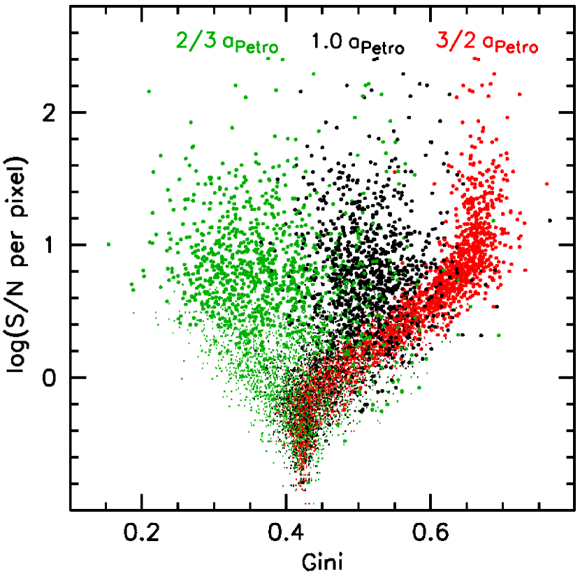
Figure 1.— Gini for different apertures. Logarithmic signal-to-noise ratio per pixel in UDF, measured within the Petrosian aperture, versus the Gini coefficient of the galaxies in UDF. Gini is shown for the three different apertures: $a=2/3\,a_{\rm Petro}$ (green or grey symbols), $a=1\,a_{\rm Petro}$ (black), and $a=3/2\,a_{\rm Petro}$ (red or grey). Large symbols represent the galaxies in the good quality subsample, i.e., having $a_{\rm Petro}\geq 10$ pixels and $m_{i}\leq 26.7$ mag. Small symbols are used for the other galaxies. For a given galaxy, the $S/N$ per pixel is defined as the average flux per pixel, divided by the noise RMS value calculated in a box centered on the galaxy’s position.

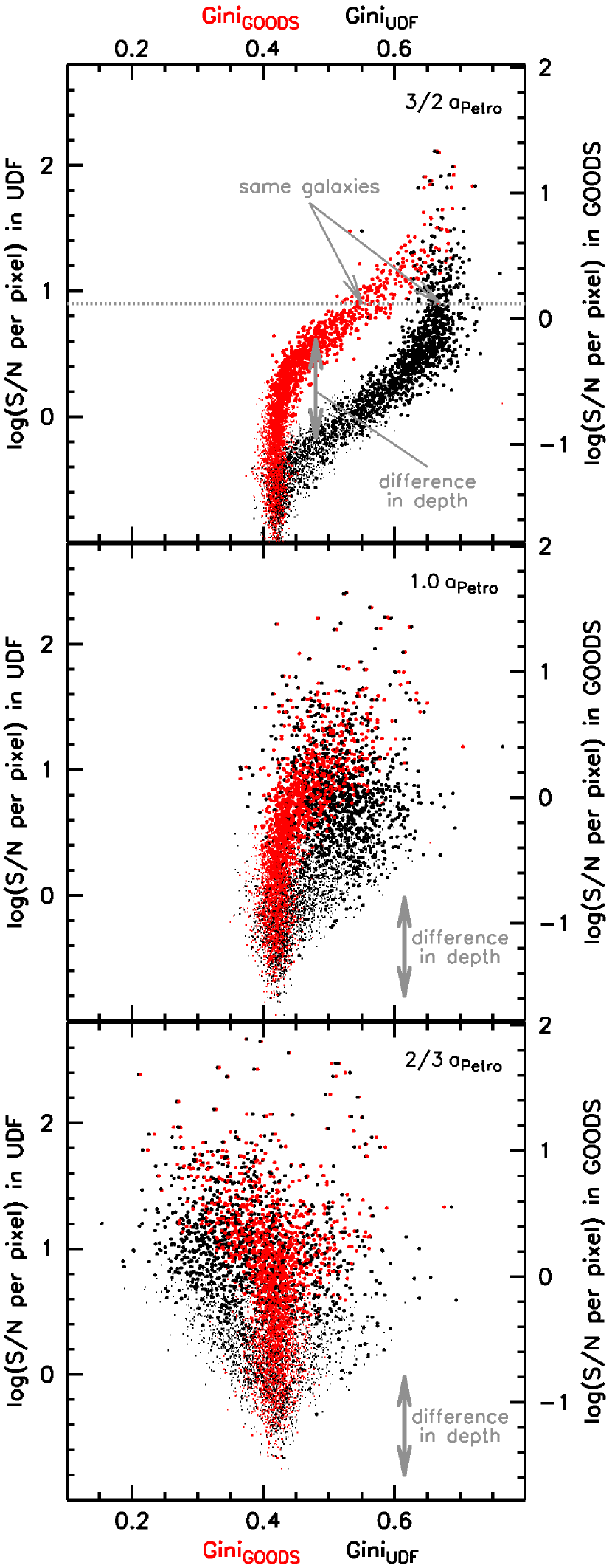
Figure 2.— Gini for different image depth. Logarithmic signal-to-noise ratio per pixel versus the Gini coefficient of the same galaxies in UDF (black symbols) and GOODS (red or white). Top: 1.5-Petrosian aperture, middle: Petrosian aperture, bottom: 2/3-Petrosian aperture. The median difference between the noise RMS of UDF and GOODS is indicated as arrow in each panel. For a given galaxy, the Gini values of UDF and GOODS lie on a horizontal line in each panel, since the galaxy’s $S/N$ value in UDF (left ordinate) was used for plotting, whereas the right ordinate has simply been scaled according to the depth difference to represent the GOODS $S/N$ values.

The strong dependence of the Gini coefficient on the aperture within which it is measured is shown in Fig. 1. For each of the three apertures, Gini occupies a completely different range of values for galaxies with a reasonably high $S/N$. The importance of this aperture dependence becomes clear when considering the fact that different authors keep using different apertures in their computation of model-independent morphology measurements: while, for example, Conselice (2003) and Conselice et al. (2000, 2008) use 1.5 circular Petrosian radii, Lotz et al. (2004, 2006, 2008) use 1.0 Petrosian SMA.

Moreover, the figure implies a $S/N$-dependence of the Gini coefficient: from the high-$S/N$ values, a transition is observed towards a common Gini value of 0.42 for all apertures at very low $S/N$, where noise dominates over the actual signal. However, from Fig. 1 alone it is not possible to judge whether this transition is a direct dependence on $S/N$, or whether it simply means that the Gini coefficient takes a different value for galaxies of different surface brightness, which could be useful to distinguish between different galaxy classes.

Consequently, a direct examination of the effects of image depth is necessary. It is made possible through a comparison of the very same galaxies and apertures in the UDF and GOODS images, which differ only by the total exposure time. This comparison is shown in Fig. 2 for the three different apertures. The arrow in each panel indicates the difference in depth between UDF and GOODS (1.95 mag), calculated from the median of the individual noise RMS measurements. For a given galaxy, the Gini values of UDF and GOODS lie on a horizontal line in each panel, since the galaxy’s $S/N$ value in UDF (left ordinate) was used for plotting, whereas the right ordinate has simply been scaled according to the depth difference to represent the GOODS $S/N$ values.

Obviously, the depth difference equals the offset of the Gini distributions for the two images. For the example of the 1.5-Petrosian aperture (top panel in Fig. 2), this means that the transition of Gini values from $\sim 0.65$ to $\sim 0.4$ is determined solely by the $S/N$, and not by different surface brightnesses of galaxies — the latter do not change between UDF and GOODS. Similar structures, though not as clearly defined, can be seen for the Petrosian and the 2/3-Petrosian aperture (middle and bottom panel). Gini thus shows a strong dependence on the $S/N$ of an image.

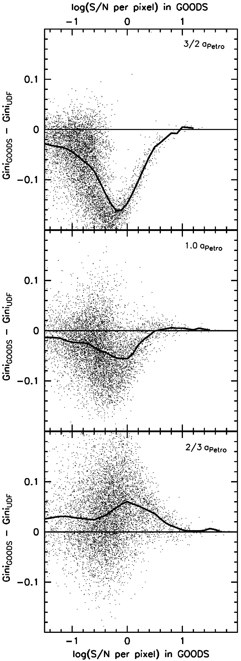
Figure 3.— Gini versus $S/N$. Logarithmic signal-to-noise ratio per pixel in GOODS versus the difference of the Gini coefficient in GOODS and UDF. The black line gives the average Gini difference. Top: 1.5-Petrosian aperture, middle: Petrosian aperture, bottom: 2/3-Petrosian aperture.

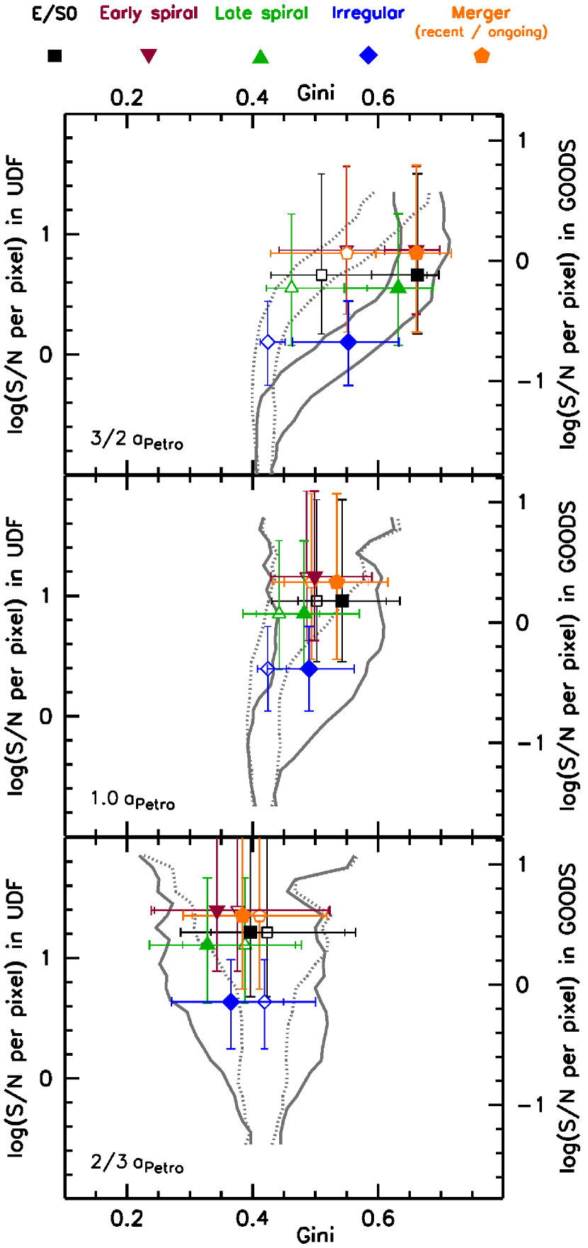
Figure 4.— Gini for different galaxy classes. Logarithmic signal-to-noise ratio per pixel versus the Gini coefficient for different galaxy classes (see text), as indicated above the diagram. Shown are the median values in UDF (filled symbols) and GOODS (open symbols); error bars represent the 5th and 95th percentile. Contours indicate the 5%-to-95% range of Gini values (cf. Fig. 2) in UDF (grey solid lines) and GOODS (grey dotted lines). For a given galaxy class, the Gini values of UDF and GOODS lie on a horizontal line in each panel, since the UDF values (left ordinate) were used for plotting, whereas the right ordinate has simply been scaled according to the depth difference to represent the GOODS $S/N$ values. Top: 1.5-Petrosian aperture, middle: Petrosian aperture, bottom: 2/3-Petrosian aperture.

In order to have a more quantitative measure of the systematic $S/N$ effect on the Gini coefficient, Fig. 3 shows the difference between the GOODS and the UDF Gini value for each galaxy, versus the $S/N$. The same comparison was presented by Lotz et al. (2006) for their sample and aperture. From this, they decided to restrict their analysis to galaxies with $S/N$ per pixel of $S/N_{p.p.}\gtrsim 2.5$ in GOODS, corresponding to $log(S/N_{p.p.})\gtrsim 0.4$. This is in agreement with the middle panel of Fig. 3, which illustrates that the difference between the GOODS and the UDF values for the Petrosian aperture is very small at this $S/N$ level.

The Gini distributions of different galaxy classes in GOODS and UDF are shown in Fig. 4, again for the three elliptical apertures. Galaxy classification was done visually for all 1019 objects with $a_{\rm Petro}\geq 10$ pixels and $m_{i}\leq 26.7$ mag, hereafter referred to as the good quality subsample. Since many, if not most galaxies in deep surveys such as UDF are not well represented by any class of the Hubble scheme, a number of additional classes can be defined that are a more “honest” representation of the diversity of galaxies at higher redshifts, such as chain galaxies, clump clusters (see Elmegreen et al., 2004b, a), and compact or high-surface brightness irregular galaxies. While this detailed classification will be used for future projects, the intention here is to get an idea of how the standard galaxy classes distribute (see the discussion), along with the combined class of candidates for ongoing and recent mergers. Therefore, only these are shown in the figure, with their median value and the corresponding interval that reaches from the 5th to the 95th percentile.

It can be seen that E/S0 galaxies and possible mergers, which typically have comparably high surface brightnesses, have similar Gini values. Recall that Gini is not sensitive to the actual location of galaxy pixels; thus, any asymmetry or irregularity in the spatial distribution does not enter the Gini calculation. Early-type spirals have a lower value at least for the 2/3-Petrosian and the Petrosian aperture, and late-type spirals have again somewhat lower values. The irregulars have a significantly lower $S/N$ on average, causing their comparison with the other classes to be affected strongly by $S/N$ effects: their Gini values are larger than those of the spirals for the 2/3-Petrosian aperture (bottom panel of Fig. 4), about equal for the Petrosian aperture (middle), and significantly lower for the 1.5-Petrosian aperture (top). As an aside, note the large overlap of all galaxy types for all apertures — while it might be possible to perform “non-parametric” quantitative galaxy classification in a statistical way, it is barely possible to obtain clean samples of each galaxy class.

4. Discussion

4.1. Merger selection

Determining the frequency of major galaxy mergers at different epochs is a crucial step towards understanding the origin of present-day massive galaxies. In this context, Lotz et al. (2008) identified mergers within the parameter space of the Gini coefficient $G$ and $M_{20}$ (which measures the distribution of the brightest 20% of a galaxy’s pixels, see Lotz et al., 2004) by selecting galaxies with $G>-0.14\cdot M_{20}+0.33$. However, Conselice et al. (2008) noted that, when applying this criterion to their galaxy sample, the majority of selected objects actually appear to be normal galaxies according to their CAS (concentration, asymmetry, clumpiness) classification criteria. They concluded that the Gini/$M_{20}$ criterion might not be selecting true mergers, or might be more sensitive to specific merger phases.

From the analysis presented here, it is immediately clear that this apparent discrepancy is caused by the strong dependence of Gini on the chosen aperture: while Lotz et al. (2008) used 1.0 Petrosian SMA, Conselice et al. (2008) chose 1.5 Petrosian radii for their aperture. Since the average Gini value increases significantly with increasing aperture (Fig. 1), Conselice et al.’s application of the Gini/$M_{20}$ criterion selected many more objects as “mergers” than it would have with Lotz et al.’s aperture. Furthermore, while Lotz et al. (2008) used elliptical apertures in order to avoid the inclusion of many noise-dominated pixels (Lotz et al., 2004), Conselice et al. (2008) used circular apertures, thereby again increasing the average Gini values of their galaxies.

Conselice et al. quote an average Gini value of 0.71 for their UDF galaxy sample, measured in the $z_{850}$ band. In the present study, the average value for the circular aperture of the same size, but measured in $i_{775}$, is 0.64, using only the good quality subsample. The corresponding values for the elliptical apertures are 0.38 for the 2/3-Petrosian aperture, 0.52 for the Petrosian aperture, and 0.62 for the 1.5-Petrosian aperture.

4.2. Choice of aperture

The signal-to-noise ratio of a galaxy is intrinsically tied to its surface brightness. Nevertheless, as emphasized in Sect. 3, the systematic change of the Gini coefficient from high to low $S/N$ values when considering the 1.5-Petrosian aperture is a true $S/N$-effect (see Fig. 2) and is not caused by varying surface brightness. This, in turn, means that each $S/N$ level defines its own specific range of possible Gini values that galaxies at this $S/N$ level can take. Therefore, a galaxy could only be properly compared to other galaxies if those are at about the same $S/N$ level — a rather alarming result. However, as can be seen from Fig. 2, this effect is far less strong for the 2/3-Petrosian and the Petrosian aperture. For these apertures, the range of Gini values covered by different galaxies is much larger with respect to the systematic $S/N$-effect — although the latter is still clearly recognizable through the difference in depth between UDF and GOODS.

The maximum systematic deviation of the Gini value that one finds acceptable can of course be subjective. Since the Gini coefficient is intended to be used to measure galaxy morphology, a useful criterion would seem that the separation between different galaxy classes be larger than the systematic $S/N$ effect. An acceptable limit for the systematic $S/N$ effect can, for example, be defined as half the difference between the median Gini values of E/S0s and late-type spirals in UDF (see Fig. 4). This would be 0.035 for the 2/3-Petrosian aperture, 0.03 for the Petrosian aperture, and 0.015 for the 1.5-Petrosian aperture. The corresponding $S/N$-restrictions from Fig. 3 would then be $log(S/N_{p.p.})\gtrsim 0.5$ for the 2/3-Petrosian aperture, $log(S/N_{p.p.})\gtrsim 0.2$ for the Petrosian aperture, and $log(S/N_{p.p.})\gtrsim 0.7$ for the 1.5-Petrosian aperture. When taking into account the effects of drizzling on the noise in GOODS (Casertano et al., 2000; Lotz et al., 2006), these limits would decrease by 0.2. Note that the $S/N$ values are calculated as the average $S/N$ of all pixels within a given aperture — it is therefore easier to obtain a larger $S/N$ value for smaller apertures, which contain fewer faint pixels.

The clear conclusion is that for the vast majority of galaxies, the Gini coefficient is strongly affected by the $S/N$ when using the 1.5-Petrosian aperture: for the GOODS images, only 2% of the galaxies in the good quality subsample meet the above criterion. For the 2/3-Petrosian and the Petrosian aperture, this fraction is significantly larger, namely 24% and 30%, respectively. It is therefore recommended to use the Petrosian aperture for calculating the Gini coefficient, confirming the approach of Lotz et al. (2004, 2006).

4.3. Assessment of previous studies

With the criteria established above, it is possible to assess whether past studies that used the Gini coefficient for galaxy classification might have been significantly affected by its systematic behaviour with $S/N$. As mentioned already in Sect. 3, in their studies of intermediate and high redshift galaxy morphology and merger fractions, Lotz et al. (2006, 2008) selected objects having $log(S/N_{p.p.})\gtrsim 0.4$ within the Petrosian aperture, for which there is almost no difference between the Gini values in GOODS and UDF (Fig. 3, middle panel). The same selection was adopted by Pierce et al. (2007) in their study of AGN host galaxy morphologies.

The study of Conselice et al. (2008) of galaxy structures and merger fractions in UDF used galaxies with $z_{850}<27.0$ mag, and adopted a circular aperture of 1.5 Petrosian radii, as mentioned previously. When requiring that the above criterion of $log(S/N_{p.p.})\gtrsim 0.7$ for the 1.5-Petrosian aperture in $i_{775}$ be met by more than 50% of the galaxies with magnitudes similar to the limiting magnitude, the latter would have to be approximately $i_{775}\leq 24.5$ mag (and leave only very few galaxies in a so selected sample). Depending on galaxy type and color, the limiting magnitude in $z_{850}$ would differ by several tenths of a magnitude, but still be more than two magnitudes brighter than the selection of Conselice et al. (2008). Consequently, the Gini values that Conselice et al. obtained for the majority of their sample must be regarded as being strongly affected by $S/N$ effects. If they had chosen the Petrosian aperture instead, the above criterion of $log(S/N_{p.p.})\gtrsim 0.2$ would have been met by about 80% of galaxies with magnitudes around $i_{775}\leq 27.0$. Furthermore, it needs to be pointed out again that their application of the merger selection criterion of Lotz et al. (2008) – which had been established for the elliptical Petrosian aperture – is heavily biased by the strong aperture dependence of the Gini coefficient (see Sect. 3 and Fig. 1), thus providing a straightforward explanation for the apparently very different sensitivity of the CAS merger selection and the Gini/$M_{20}$ merger selection (cf. Conselice et al., 2008).

The Gini coefficient was used by Neichel et al. (2008) in their analysis of intermediate-mass galaxies at redshift $z\approx 0.6$. These authors find good agreement of visual morphological classification with the dynamical states of the galaxies, but point out that this correlation is not as clear when using automated classification methods instead. With the Petrosian aperture and a limiting magnitude of $i_{775}=23.5$ mag for GOODS images, they are only weakly affected by $S/N$ effects: about 20% of galaxies with magnitudes around $i_{775}=23.5$ mag fall below the $S/N$ criterion. The $S/N$ effect on the Gini coefficient can cause low-$S/N$ objects to be assigned to later galaxy types than they actually belong to (cf. Fig. 4), or mergers to fall out of the merger regime as defined by Lotz et al. (2008) and used by Neichel et al. (2008). This could partly explain that the visually assigned classes of Neichel et al. intermingle when using the Gini/$M_{20}$ criterion, but only few of their 52 galaxies should be affected by this.

Urrutia et al. (2008) applied the Gini coefficient in their analysis of quasar host galaxies, following the Gini calculation of Lotz et al. (2004). Their $I_{814}$ HST/ACS imaging exposure times are $\lesssim 30$ times lower than the total exposure time of GOODS $i_{775}$, corresponding to a difference in depth of $\lesssim 1.8$ mag. Since all galaxies of their sample have magnitudes $I_{814}<21$ mag, their study does not suffer from $S/N$ effects on the Gini values.

Based on COSMOS (Scoville et al., 2007b) HST/ACS data, Capak et al. (2007) and Casey et al. (2008) applied the Gini coefficient to study the evolution of the morphology-density relation, and to morphologically select faint AGN, respectively. Both rely on the Gini calculation outlined in Abraham et al. (2007), using a “quasi-Petrosian” aperture. A magnitude limit of $I_{814}<24$ mag is used by Capak et al. (2007), whereas Casey et al. (2008) adopt $I_{814}<24.5$ mag. Due to the larger pixel scale of the COSMOS data as compared to GOODS, a galaxy would actually have a slightly larger $S/N$ per pixel in COSMOS than in GOODS, despite the shallower depth of COSMOS (Scoville et al., 2007a).

Taking this into account, $\sim$30% of galaxies with magnitudes close to the limit of Capak et al. (2007) fall below the $S/N$ criterion established above, and $\sim$15% of all galaxies brighter than the limit would do so. These authors separated early and late-type galaxies according to their Gini value, and therefore probably missed a certain fraction of (faint) early types. Since mostly galaxies at higher redshift should be affected, due to their lower overall $S/N$, the growth rate of the early-type fraction with cosmic time determined by Capak et al. may have been slightly overestimated.

For the study of Casey et al. (2008), $\sim$35% of galaxies close to the magnitude limit do not meet the $S/N$ criterion, and $\sim$20% of all galaxies brighter than the limit do so. They applied the Gini coefficient to select compact sources that are likely to be AGNs by their high Gini value. Therefore, the authors might have missed a small fraction of galaxies at low $S/N$ levels with Gini values close to the selection limit, which would have entered their AGN candidate sample at larger $S/N$.

The fractions of $S/N$-affected galaxies given above for the study of Capak et al. (2007) also apply to the COSMOS morphological classification presented by Scarlata et al. (2007). This leads to a certain number of (faint) galaxies being classified as later types than they should, and is in agreement with Scarlata et al.’s estimate that $\lesssim 30\%$ of faint early types could be misclassified as disks or irregulars.

In their study of the morphology of distant star-forming galaxies in COSMOS, Zamojski et al. (2007) adopt a magnitude limit of $I_{814}<23$ mag, thus avoiding any significant $S/N$ effect. Likewise, the selection of $I_{814}<22$ mag for COSMOS and $i_{775}<22$ mag for GOODS ensured that no $S/N$ effect on the Gini values affected the morphological analysis of Lisker et al. (2006), who presented a preliminary method for identifying bars based on radial Gini profiles.

Abraham et al. (2007) stated that “the Gini coefficient remains a surprisingly robust statistic, even in the face of morphological $K$-corrections”. This was based on their assessment of the robustness of the Gini coefficient (computed within the “quasi-Petrosian” aperture), using an SDSS reference sample of nearby galaxies for their HST/ACS study of distant early-type galaxies. The galaxies in both their HST/ACS sample and their SDSS reference sample have a total $S/N>100$. When compared to the GOODS data of the present study, indeed all galaxies with $S/N>100$ would meet the $S/N$-criterion established above, in accordance with Abraham et al.’s positive conclusion on the performance of the Gini coefficient as morphology estimator.

5. Concluding remarks

So far, most authors using the Gini coefficient to describe galaxy morphology applied a reasonable magnitude and/or $S/N$ selection that prevented their investigations from being seriously affected by $S/N$ effects. However, I have shown that the Gini coefficient depends strongly on the aperture within which it is computed, and that it exhibits a strong dependence on $S/N$ below a certain $S/N$ level (which, again, depends on the aperture). Therefore, quantitative selection criteria involving the Gini coefficient – such as the merger selection of Lotz et al. (2008) – cannot be straightforwardly applied to a different dataset than the one for which they have been established (cf. Conselice et al., 2008). Care needs to be taken with the selection of aperture and limiting magnitude, as well as with the comparison of calculated Gini values to those of other studies. From the analysis presented here, the use of the Petrosian aperture is recommended. Larger apertures are strongly disfavored due to their inclusion of many faint pixels.

Typically, the total $S/N$ or the $S/N$ per pixel are quoted as quantitative, but crude estimates of the “quality” of a galaxy’s image. From these average values, it can of course not be seen whether a given galaxy image actually consists of pixels with very different individual $S/N$ values, or whether the $S/N$ of most pixels is similar — which might make a huge difference depending on the desired analysis. This pixel flux distribution is exactly what the Gini coefficient, by definition, measures. One could thus conclude somewhat ironically that the Gini coefficient could serve as a sophisticated measure of the $S/N$ distribution within a galaxy’s image, if it did not depend so much on the galaxy’s morphology.

References

- Abraham et al. (2007) Abraham, R. G., et al. 2007, ApJ, 669, 184
- Abraham et al. (1996a) Abraham, R. G., Tanvir, N. R., Santiago, B. X., Ellis, R. S., Glazebrook, K., & van den Bergh, S. 1996a, MNRAS, 279, L47
- Abraham et al. (1994) Abraham, R. G., Valdes, F., Yee, H. K. C., & van den Bergh, S. 1994, ApJ, 432, 75
- Abraham et al. (1996b) Abraham, R. G., van den Bergh, S., Glazebrook, K., Ellis, R. S., Santiago, B. X., Surma, P., & Griffiths, R. E. 1996b, ApJS, 107, 1
- Abraham et al. (2003) Abraham, R. G., van den Bergh, S., & Nair, P. 2003, ApJ, 588, 218
- Beckwith et al. (2006) Beckwith, S. V. W., et al. 2006, AJ, 132, 1729
- Bell et al. (2006a) Bell, E. F., et al. 2006a, ApJ, 640, 241
- Bell et al. (2006b) Bell, E. F., Phleps, S., Somerville, R. S., Wolf, C., Borch, A., & Meisenheimer, K. 2006b, ApJ, 652, 270
- Bell et al. (2004) Bell, E. F., et al. 2004, ApJ, 608, 752
- Bershady et al. (2000) Bershady, M. A., Jangren, A., & Conselice, C. J. 2000, AJ, 119, 2645
- Capak et al. (2007) Capak, P., Abraham, R. G., Ellis, R. S., Mobasher, B., Scoville, N., Sheth, K., & Koekemoer, A. 2007, ApJS, 172, 284
- Casertano et al. (2000) Casertano, S., et al. 2000, AJ, 120, 2747
- Casey et al. (2008) Casey, C. M., et al. 2008, ApJS, 177, 131
- Coe et al. (2006) Coe, D., Benítez, N., Sánchez, S. F., Jee, M., Bouwens, R., & Ford, H. 2006, AJ, 132, 926
- Conselice (1997) Conselice, C. J. 1997, PASP, 109, 1251
- Conselice (2003) —. 2003, ApJS, 147, 1
- Conselice et al. (2003a) Conselice, C. J., Bershady, M. A., Dickinson, M., & Papovich, C. 2003a, AJ, 126, 1183
- Conselice et al. (2000) Conselice, C. J., Bershady, M. A., & Jangren, A. 2000, ApJ, 529, 886
- Conselice et al. (2003b) Conselice, C. J., Chapman, S. C., & Windhorst, R. A. 2003b, ApJ, 596, L5
- Conselice et al. (2008) Conselice, C. J., Rajgor, S., & Myers, R. 2008, MNRAS, 446
- Cowie et al. (1995a) Cowie, L. L., Hu, E. M., & Songaila, A. 1995a, Nature, 377, 603
- Cowie et al. (1995b) —. 1995b, AJ, 110, 1576
- Elmegreen et al. (2004a) Elmegreen, D. M., Elmegreen, B. G., & Hirst, A. C. 2004a, ApJ, 604, L21
- Elmegreen et al. (2004b) Elmegreen, D. M., Elmegreen, B. G., & Sheets, C. M. 2004b, ApJ, 603, 74
- Ferreras et al. (2005) Ferreras, I., Lisker, T., Carollo, C. M., Lilly, S. J., & Mobasher, B. 2005, ApJ, 635, 243
- Giavalisco et al. (2004) Giavalisco, M., et al. 2004, ApJ, 600, L93
- Gini (1912) Gini C., 1912, reprinted in Memorie di Metodologia Statistica, ed. E. Pizetti & T. Salvemini (1955; Rome: Libreria Eredi Virgilio Veschi)
- Graham et al. (2001) Graham, A. W., Trujillo, I., & Caon, N. 2001, AJ, 122, 1707
- Kornreich et al. (1998) Kornreich, D. A., Haynes, M. P., & Lovelace, R. V. E. 1998, AJ, 116, 2154
- Lisker et al. (2006) Lisker, T., Debattista, V. P., Ferreras, I., & Erwin, P. 2006, MNRAS, 370, 477
- Lisker et al. (2007) Lisker, T., Grebel, E. K., Binggeli, B., & Glatt, K. 2007, ApJ, 660, 1186
- Lotz et al. (2008) Lotz, J. M., et al. 2008, ApJ, 672, 177
- Lotz et al. (2006) Lotz, J. M., Madau, P., Giavalisco, M., Primack, J., & Ferguson, H. C. 2006, ApJ, 636, 592
- Lotz et al. (2004) Lotz, J. M., Primack, J., & Madau, P. 2004, AJ, 128, 163
- Madau et al. (1998) Madau, P., Pozzetti, L., & Dickinson, M. 1998, ApJ, 498, 106
- Neichel et al. (2008) Neichel, B., et al. 2008, A&A, 484, 159
- Petrosian (1976) Petrosian, V. 1976, ApJ, 209, L1
- Pierce et al. (2007) Pierce, C. M., et al. 2007, ApJ, 660, L19
- Scarlata et al. (2007) Scarlata, C., et al. 2007, ApJS, 172, 406
- Schawinski et al. (2007) Schawinski, K., Thomas, D., Sarzi, M., Maraston, C., Kaviraj, S., Joo, S.-J., Yi, S. K., & Silk, J. 2007, MNRAS, 382, 1415
- Scoville et al. (2007a) Scoville, N., et al. 2007a, ApJS, 172, 38
- Scoville et al. (2007b) Scoville, N., et al. 2007b, ApJS, 172, 1
- Sérsic (1963) Sérsic, J. L. 1963, Boletin de la Asociacion Argentina de Astronomia La Plata Argentina, 6, 41
- Stoughton et al. (2002) Stoughton, C., et al. 2002, AJ, 123, 485
- Trujillo et al. (2001) Trujillo, I., Graham, A. W., & Caon, N. 2001, MNRAS, 326, 869
- Urrutia et al. (2008) Urrutia, T., Lacy, M., & Becker, R. H. 2008, ApJ, 674, 80
- Zamojski et al. (2007) Zamojski, M. A., et al. 2007, ApJS, 172, 468