A Parameter Study of Classical Be Star Disk Models Constrained by Optical Interferometry

Abstract

We have computed theoretical models of circumstellar disks for the classical Be stars $\kappa$ Dra, $\beta$ Psc, and $\upsilon$ Cyg. Models were constructed using a non-LTE radiative transfer code developed by Sigut & Jones (2007) which incorporates a number of improvements over previous treatments of the disk thermal structure, including a realistic chemical composition. Our models are constrained by direct comparison with long baseline optical interferometric observations of the H$\alpha$ emitting regions and by contemporaneous H$\alpha$ line profiles. Detailed comparisons of our predictions with H$\alpha$ interferometry and spectroscopy place very tight constraints on the density distributions for these circumstellar disks.

1 Introduction

Classical Be (or B-emission) stars are rapidly rotating, hot stars with optical spectra that show hydrogen emission lines, and, frequently, emission lines from singly ionized metals. It has been recognized since the days of Struve (1931) that recombination in a flattened disk of circumstellar gas can reproduce the basic features of the spectroscopically observed H$\alpha$ line profiles of Be stars. However, it is now generally accepted that this model is too simplistic. The detailed mechanism(s) that creates and maintains Be star disks remains unclear (Porter & Rivinus, 2003; Owocki, 2003), although rapid rotation of the central B star certainly plays a role (Townsend et al., 2004). In addition to this lack of a successful dynamical model, the evolutionary status of Be stars and related stars (such as B[e] stars) is not well understood, and possible evolutionary connections between these groups are ambiguous. These problems are compounded by the additional uncertainty in their rotation rates (Cranmer, 2005; Townsend et al., 2004; Owocki, 2003) and lack of understanding of how rotation and evolution interplay. The suggestion by Townsend et al. (2004) that the rotation rates of Be stars may be systematically underestimated, combined with new interferometric data, has rekindled interest in finding suitable dynamical models for these stars.

Until recently, the bulk of the observational evidence for the presence of disks surrounding Be stars has been spectroscopic and polarimetric in nature. The spectroscopic evidence includes the profiles of the emission lines observed in the optical and IR spectra, as well as continuum excesses at infrared wavelengths. The net linear polarization observed in Be stars arises via electron scattering in the non-spherical distribution of gas, as first suggested by Coyne & Kruszewski (1969). However, interferometric observations that spatially resolve the disks in several wavelength regimes are becoming available, (see for example Chesneau et al., 2005; McAlister et al., 2005; Tycner et al., 2006). Interferometric observations, in concert with other observables, allow the disk physical properties to be determined with greater accuracy and this may contribute to the development of more successful dynamical models.

Tycner et al. (2006) collected long-baseline, optical, interferometric observations of the classical Be stars $\gamma\;$Cas and $\phi\;$Per at the Navy Prototype Optical Interferometer (NPOI) and interpreted these observations using simple models of the intensity distribution on the sky, such as uniform disks, rings, or disks with a Gaussian intensity distribution. In this paper, we extend the work of Tycner et al. (2006) by computing detailed theoretical models for the intensity distribution on the sky produced by the central B star and disk of a Be system. We then compare these models to observations collected at the NPOI.

The theoretical models are computed with the bedisk code developed by Sigut & Jones (2007). Assuming a density distribution of the disk gas, the code can compute the temperatures in the disk given the energy input from the central stars’ photoionizing radiation field, by enforcing radiative equilibrium. As the disk density model contains several adjustable parameters, values for these parameters can then be extracted from the match to observations. We present new observations and detailed models for the Be stars $\kappa\;$Dra, $\beta\;$Psc, and $\upsilon\;$Cyg. We also use near-contemporaneous observations of the H$\alpha$ spectral lines for these stars as additional constraints on the density model. As we shall demonstrate, the additional spectroscopic constraint of detailed line profiles is often an important ingredient in selecting among models consistent with the interferometric observations. The overall goal of this study is to place tight constraints on physical conditions in the circumstellar regions of these Be stars.

2 Theory

The theoretical disk models presented in this investigation were constructed using the bedisk code developed by Sigut & Jones (2007). A brief overview of the code and assumptions relevant to this work are presented below. The reader is referred to Sigut & Jones (2007) for more details.

The circumstellar disk is assumed to be axi-symmetric about the star’s rotation axis and symmetric about the mid-plane of the disk. In this case, cylindrical geometry is appropriate and we use $R$ for the radial distance from the star’s rotation axis and $Z$ for the height above the equatorial plane. The radial density distribution in the equatorial plane is assumed to be given by an $R^{-n}$ power-law following the works of Waters (1986); Coté & Waters (1987); Waters & Coté (1987). At each radial distance from the rotation axis, the vertical structure of the disk is determined by the requirement of hydrostatic equilibrium in the $Z$ direction which balances the $Z$ component of the star’s gravitational acceleration with the gradient of the gas pressure.

Typical values for the radial power-law index $n$ for theoretical models of Be stars usually fall in the range of 2 to 3.5 based on models that fit the IR continuum (Waters, 1986). Models with the highest values of $n$ have a faster decrease in the density distribution with increasing $R$. The density distribution within the disk is determined by an assumed value of the density at the stellar surface in the equatorial plane, $\rho_{\circ}$, by the power-law index, $n$, and by the assumption of pressure support perpendicular to the equatorial plane. Since $\rho_{\circ}$ and $n$ significantly affect the theoretical predictions, we conduct a 2-dimensional parameter search by varying these input parameters over all reasonable values for comparison with interferometric and spectroscopic observations.

Given this density model, the bedisk code is used to find the temperature structure of the disk by enforcing radiative equilibrium. The microscopic heating and cooling rates implied by a gas with a solar chemical composition are computed and the temperature that balances heating and cooling is found. To compute the atomic level populations required by this procedure, the statistical equilibrium equations are solved for each chemical element included, accounting for the bound-bound and bound-free collisional and radiative processes that set the rates in and out of each atomic level.

To compute the hydrogen line profiles, we solved the transfer equation along a series of rays through the star plus disk system as viewed at an angle $i$ relative to the line-of-sight (where $i=0^{o}$ is pole-on, and $i=90^{o}$ is equator-on). The disk is assumed to be in pure Keplerian rotation, and the equatorial rotational velocity of the star was chosen so that the measured $v\sin i$ of the star was recovered for the adopted value of $i$. For rays terminating on the stellar surface, we adopted a photospheric H$\alpha$ line profile computed using the synthe code and the Stark Broadening routines of Barklem & Piskunov (2003); these profiles are based on the hydrogen populations computed for the appropriate LTE, line-blanketed model atmosphere adopted from Kurucz (1993). For rays passing through the disk, the equation of radiative transfer was solved along the ray using the short-characteristics method of Olson & Kunasz (1987). To compute the H$\alpha$ opacity and emissivity, the hydrogen level populations computed for the thermal solution were used. Here, hydrogen was represented by a 15 level atom and all implied radiative and collisional bound-bound and bound-free processes from and between the 15 levels were included. The radiative bound-bound rates were treated by the escape probability approximation in which the net radiative bracket for the line (Mihalas, 1978) is replaced by a single-flight escape probability. While the escape probability approximation can provide a reasonable description of the line thermalization, the use of escape probabilities is an important approximation. The bedisk code assumes static escape probabilities based on the complete redistribution over a Doppler profile for all lines (for a justification of this procedure see Sigut & Jones, 2007). If the functional form of the escape probability function is changed, for example, to a simple $\tau^{-1}$ dependence on optical depth for $\tau\gg 1$, the predicted equivalent width of H$\alpha$ can change by $\sim\,2$ Å  (due to the change in the thermal structure of the disk and in the hydrogen level populations). Thus in matching to the observed H$\alpha$ profiles, the largest uncertainty is likely from the uncertainty in the theoretical profile and not from the observational uncertainties (see Section 3 for an estimate of the observational uncertainties).

Our approach allows the full dependence of the H$\alpha$ line emissivity and opacity on the physical conditions throughout the disk to be retained. The Stark broadening routines of Barklem & Piskunov (2003) were also used to compute the local H$\alpha$ line profile throughout the disk. This is important as these routines can handle high disk densities for which the assumption of a simple Gaussian or Voigt profile for the H$\alpha$ line would be invalid. The final H$\alpha$ line profile from the unresolved system was obtained by summing over the rays weighted by their projected area on the sky. The H$\alpha$ line profile was computed over a wavelength bin of $\pm 20$Å from line centre at each area element on the sky. To obtain the final H$\alpha$ line profile to compare with spectroscopic observations, the profile was convolved with a Gaussian of FWHM of $0.656\,$Å to bring the resolving power of the computed profile down to $10^{4}$ to match the observations. The predicted interferometric visibilities also followed from the same numerical model. The monochromatic H$\alpha$ image of the system projected on the plane of the sky was computed by integrating the stellar continuum and H$\alpha$ line flux over a 150 Å  spectral window centered at H$\alpha$ to represent the interferometric spectral channels (see Section 3). Thus the calculation of the H$\alpha$ profiles and the H$\alpha$ interferometric visibilities used the same model calculations.

3 Observations

We obtained long-baseline interferometric and spectroscopic observations of three Be stars, $\kappa$ Dra, $\beta$ Psc, and $\upsilon$ Cyg. The interferometric observations were acquired using the Navy Prototype Optical Interferometer (NPOI) utilizing baselines ranging from 18.9 to 64.4 m in length. The NPOI is described in detail in Armstrong et al. (1998) and the technique used to extract interferometric observables from the spectral channel containing the H$\alpha$ emission line has been discussed by Tycner et al. (2003). Table 1 shows all the interferometric observations obtained for the three stars and the number of data points obtained on each night in the spectral channel containing the H$\alpha$ line. The interferometric observations of all stars were obtained over a period of less than a month, with $\beta$ Psc and $\upsilon$ Cyg observed during 2005, and $\kappa$ Dra observed during 2006.

To complement our interferometric observations we have also obtained near contemporaneous spectroscopic observations of all three targets. The spectroscopic observations were obtained using an Echelle spectrograph at the Lowell Observatory’s John. S. Hall telescope and covered the spectral region around the H$\alpha$ line. The properties of the spectrograph and the description of the reduction methods have been described elsewhere (see § 3.2 in Tycner et al., 2006, and references therein). The continuum signal-to-noise ratio (SNR) near H$\alpha$ is more than 200 in the spectra of all three stars. However, the equivalent width and the shape of the line is determined with respect to the normalized continuum level. Because the line profile must be normalized by a smoothly varying function that is fit to the continuum (or where one thinks the continuum is located), the choice of this normalizing function affects the shape of the H$\alpha$ line. In addition, the presence of telluric lines, as well as their temporal variability from night to night (and season to season) can affect how well the continuum level is determined; we expect this to be the dominant source of uncertainty associated with the shape of the observed H$\alpha$ line. We have estimated the magnitude of this effect by analyzing a set of reduced spectra all obtained from the same raw spectrum, but all obtained with slightly different quadratic functions fitted to slightly different continuum regions. The variations in the resulting normalized continuum were at the 2 to 3% level, and to be conservative we adopt a 3% uncertainty for our continuum level determination and, in turn, the shape and equivalent width measure of the observed H$\alpha$ emission line.

For $\beta$ Psc and $\upsilon$ Cyg the spectra were obtained on 2005 Sep 16, and for $\kappa$ Dra the spectrum was obtained on 2006 Mar 17, and therefore in all three cases the spectroscopic observations overlapped the interferometric observing runs (Table 1). The equivalent widths of the observed H$\alpha$ spectra lines are -15.3 Å, -24.8 Å, and -22.2 Å  for $\beta$ Psc, $\upsilon$ Cyg, and $\kappa$ Dra, respectively. (We adopt the usual convention that a negative in the quoted value of the equivalent width indicates a net line flux above the continuum.)

Table 1: Observing Log for Interferometric Observations

UT Date	$\kappa$ Dra	$\beta$ Psc	$\upsilon$ Cyg
	(# of points)	(# of points)	(# of points)
2005 Aug 28	…	12	8
2005 Aug 29	…	16	12
2005 Aug 30	…	20	20
2005 Aug 31	…	20	20
2005 Sep 1	…	20	20
2005 Sep 5	…	8	4
2005 Sep 13	…	16	16
2005 Sep 14	…	23	20
2005 Sep 15	…	20	20
2005 Sep 16	…	21	24
2005 Sep 17	…	8	9
2005 Sep 26	…	16	28
2006 Feb 25	30	…	…
2006 Feb 26	6	…	…
2006 Mar 5	52	…	…
2006 Mar 6	24	…	…
2006 Mar 14	36	…	…
2006 Mar 16	76	…	…
2006 Mar 19	52	…	…
Total:	276	200	201

4 Results

There is considerable uncertainty in the assigned spectral types for Be stars due to rapid rotation and spectral variability. The effects of gravity darkening, and the potential obscuration of portions of the stellar surface by the disk, further compound the uncertainty in classification and the corresponding stellar parameters. Since the stellar parameters fix the photoionizing radiation field that is assumed to be the sole source of energy input into the circumstellar disk, realistic stellar parameters are essential to the construction of reasonable disk models. For each of the stars in this study, we searched the literature in order to find the most reasonable stellar parameters available. See Table 2 for the adopted stellar parameters for $\kappa$ Dra, $\beta$ Psc, and $\upsilon$ Cyg. The rationale for adopting the particular stellar parameters is explained and compared with other published values in each subsection for a given star.

Table 2: Adopted stellar parameters

Star	HR	$\log g$	Spectral	Stellar Radius	Stellar Mass	$T_{eff}$	$v\sin i$	Reference
Name	Number		Type	${\rm R}_{\odot}$	${\rm M}_{\odot}$	K	km/s
$\kappa$ Dra	HR4787	3.5	B6IIIpe	6.4	4.8	14000	170	1
$\beta$ Psc	HR8773	4.0	B6Ve	3.6	4.7	15500	90$\pm$15	2
$\upsilon$ Cyg	HR8146	4.0	B2Vne	4.7	6.8	19800	173$\pm$10	3

4.1 $\kappa$ Draconis

$\kappa$ Dra is a known spectroscopic binary and giant star of intermediate spectral type. It is variable on a variety of timescales; see Hirata (1995) for a detailed discussion of these variations. Saad (2004) modeled the central star of $\kappa$ Dra by comparing a variety of spectroscopic and photometric observations to a grid of non-LTE models. We have adopted their derived best-fit stellar parameters for our study. We used their parameters of $T_{eff}$, log$g$, and mass to calculate the stellar radius. Gies et al. (2007) also used these parameters for the interpretation of $K^{\prime}$-band observations of $\kappa\;$Dra collected at the CHARA Array interferometer. The parameters of Saad (2004) are also in reasonable agreement with stellar parameters listed for the spectral class of B5III in Cox (2000).

Figure 1: The density parameter grid for $\kappa$ Dra shown as a function of $\rho_{o}$ (g/cm³) and $n$.

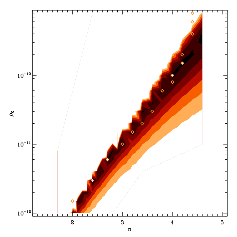
Figure 2: The $\chi^{2}$ values for computed models as a function of $n$ and $\rho_{o}$ (g/cm³) for $\kappa$ Dra. The contour plot shows the reduced $\chi^{2}$ values in steps of 1.0. Only a region of reduced $\chi^{2}<6$ is shown. The darkest regions on the figure represent models with reduced $\chi^{2}<2$. The four white plus signs correspond to models with the lowest values of reduced $\chi^{2}$ determined from interferometry. The diamonds correspond to models that have predicted H$\alpha$ equivalent widths $\pm\,2\,$Å  of the observation.

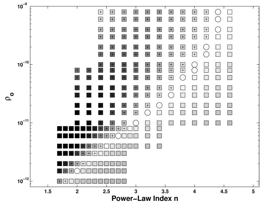
Figure 3: The predicted H$\alpha$ equivalent widths as a function of $\log\,\rho_{o}$, and the power-law index, $n$, for the entire grid of models. The lightest coloured symbols are closest to the value of the observed equivalent width of -22.2 Å . The models that predict H$\alpha$ equivalent width within $\pm\,2\,$Å  of the observation are represented by white circles. The models that correspond to predicted H$\alpha$ emission greater than the observation are indicated by the plus sign within the symbol.

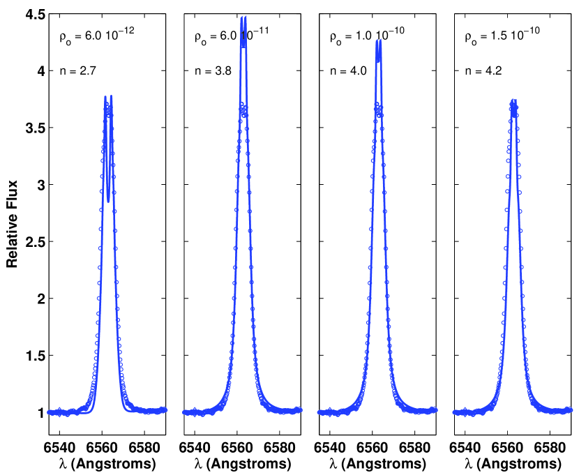
Figure 4: The observed H$\alpha$ line for $\kappa$ Dra compared with 4 models with $n$ and $\rho_{o}$ as indicated in the panels. These models correspond the best-fit from both interferometry and H$\alpha$ modeling. The model profiles are the solid lines and the circles represent the observed line. All model profiles were obtained with a disk inclination of 35^o. The reduced $\chi^{2}$ values from interferometry for these models are 1.18, 1.29, 1.18, and 1.18, from left to right respectively.

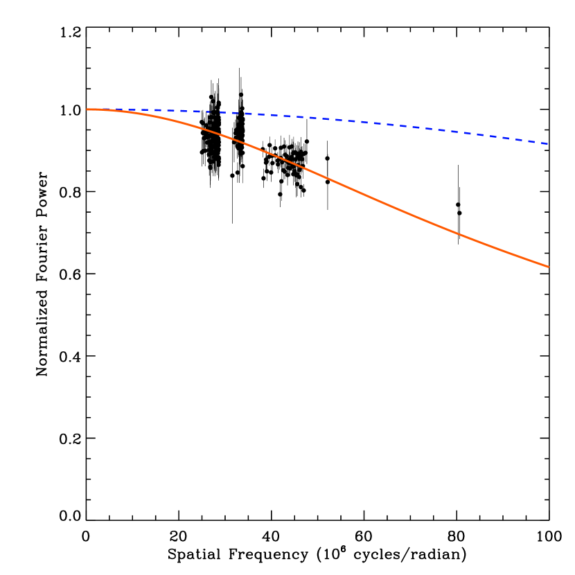
Figure 5: The interferometric data and model with $n=4.2$, and $\rho_{o}=1.5\times 10^{-10}$ g/cm³ for $\kappa$ Dra. The dashed line represents the central star and the solid line is obtained by taking a Fourier transform of a synthetic image of the preferred model.

Figure 1 shows the density parameter grid for the disk of $\kappa\;$Dra. This grid was selected after running a series of models over a much wider range in $\rho_{o}$ and $n$ on a coarser grid. A comparison of the observed and predicted H$\alpha$ equivalent widths allowed us to determine a finer grid to sample for detailed comparisons with interferometric observations. The final density parameter grid consisted of 278 models. We have compared the output from each model to the interferometric observations using the technique described in detail by Tycner et al. (2008). The reduced $\chi^{2}$ values corresponding to these models are presented in Figure 2 as a function of $\rho_{o}$ (g/cm³) and $n$. The darkest patches in this Figure represent the models with reduced $\chi^{2}<2$. The white plus signs correspond to models with the lowest values (ranging from 1.18 to 1.29) of the interferometric reduced $\chi^{2}$. In total, there are 25 models with reduced $\chi^{2}<2$ for this star, therefore, it is necessary to further constrain our models in order to determine the best-fit model.

Figure 3 shows the predicted H$\alpha$ equivalent widths as a function of $\log\,\rho_{o}$, and the power-law index, $n$, for the entire grid of models. The predicted H$\alpha$ profiles were constructed assuming an inclination of $i=35^{o}$. We note that this value of $i$ is consistent with other values determined from spectroscopy and polarization analyzes presented in the literature. For example, Clarke (1990), estimates $i=23^{o}$ based on the observed polarization angle, and Juza et al. (1991) find $i=35^{o}-45^{o}$ based on spectroscopy. We also experimented by varying $i$ and found that an inclination angle for this system of $35^{o}$ seemed to produce profiles that matched the observed H$\alpha$ line. We also note that although changing the value of $i$ by $\pm$ $10^{o}$ changes the shape of the H$\alpha$ profile, the effect on the equivalent width is $<1$ Å. The lightest coloured symbols are closest to the value of the observed equivalent width of -22.2 Å. There are 14 models that predict an H$\alpha$ equivalent width within $\pm\,2\,$ Å  of the observation and these are represented by white circles. Models which correspond to predicted H$\alpha$ equivalent widths greater than the observed emission have a plus sign within the corresponding symbol in Figure 3.

We note that this subset of 14 models does not represent the 14 best models using interferometry alone. Although this set matches the observed H$\alpha$ equivalent width within $\pm$ 2 Å, using interferometric observations as a constraint this same set corresponds to reduced $\chi^{2}$ from 1.18 (the minimum value) up to 16.0. In fact, 6 of the 14 models in this set had a reduced $\chi^{2}$ greater than 2.0. It is clear from a comparison of Figure 2 and Figure 3 that the results from H$\alpha$ interferometry and H$\alpha$ line profile are complimentary but that each provides extra information to help reduce the degeneracy in finding the best-fit model.

Multiple models, of pairs of $n$ and $\rho_{o}$, that produce H$\alpha$ profiles with equivalent widths that match the observations within uncertainties can be found. However, not all of these are the best-fits in terms of interferometry. That is, it is possible to match the equivalent width for a range of $n$ by an appropriate adjustment in $\rho_{o}$, but that these combinations do not necessary have the correct density distribution as a function of radial distance from the star. However, by combining results from spectroscopy and interferometry, we can find the best pairs of $n$ and $\rho_{o}$ for $\kappa$ Dra.

Next, we compared the subset of 8 models which represent the best-fits from both interferometry and H$\alpha$ equivalent width. A subset (4 models with the lowest reduced $\chi^{2}$ from interferometry) of the corresponding H$\alpha$ profiles is shown in Figure 4. Notice the variation in the shape of the profile as $n$ is increased from 2.7 in the left-most panel to 4.2 in the right-most panel. The predicted equivalent widths are -21.9, -23.5, -22.4, and -20.3 Å, with the corresponding $\chi^{2}$ values from interferometry of 1.18, 1.29, 1.18, and 1.18. The model with $n=2.7$ does not have the the correct line profile shape compared to the observed profile. There is too much absorption at line centre, and the profile is clearly too narrow in the wings. All of the predicted profiles in Figure 4 have an absorption feature at line centre. This feature is the most pronounced for low values of $n$ and gradually decreases for models with higher values of $n$. If we increase the inclination, this absorption feature becomes more and more pronounced as the system is viewed closer and closer to edge on. If we decrease $i$, so the system is viewed close to pole-on, the absorption feature remains for the models with the lowest values of $n$. In addition, with $n=2.7$, the wings of the predicted profile are not broad enough for any reasonable values of $i$. The panel with the model corresponding to $n=3.8$ and $n=4.0$ in Figure 4 shows that the predicted line is too strong and this results in an H$\alpha$ equivalent width which is too large. Models corresponding to $n>4.2$ have profiles with wings wider than the observation. The model that corresponds to the profile with $n=4.2$ matches the shape of the observed profile best and has a minimum reduced $\chi^{2}$ of 1.18 from interferometry. We prefer this model with $n=4.2$ and $\rho_{o}=1.5\times 10^{-10}$ g/cm³ in terms of both spectroscopy and interferometry. Figure 5 shows the interferometric observations compared with this model for $\kappa$ Dra.

We note that as previously discussed the uncertainty due to the approximations in the computational code (see Section 2) are larger than those in the observed H$\alpha$ profiles (see Section 3). We searched the literature to find the best possible stellar parameters for the disk systems studied in this investigation (see Section 4.1, 4.2, 4.3). However, generally for Be stars, not only are the stellar parameters not well established but for some stars, even the spectral type may not be accurate. We now wish to test the dependence of model parameters on our results. We experimented by varying the stellar parameters in turn, to see how these changes affect the predicted H$\alpha$ equivalent widths and the interferometric fits for the star $\kappa$ Dra. Similar types of uncertainties would be expected for the other two systems presented in this paper. One might expect that the $T_{eff}$ of the central star, which supplies the disk with energy, may be the source of the greatest uncertainty. We changed the $T_{eff}$ by $\pm$ 1000 $K$ and reproduced all of the profiles. This resulted in a change in the equivalent width of the H$\alpha$ line by a maximum of $\sim$ 2 Å. To assess the effect of uncertainties in the fundamental stellar parameters combined, we performed a Monte Carlo simulation in which new stellar parameters were randomly realized. These parameters were used to compute a new circumstellar disk model, corresponding to our preferred model of $n=4.2$ and $\rho_{o}=1.5\times 10^{-10}\;\rm{g/cm^{3}}$. This procedure was repeated to generate new H$\alpha$ profiles and equivalent widths. Errors assumed for the stellar parameters were $\pm\,25$% in mass, $\pm\,25$% in radius, and $\pm\,10.7$% in $T_{eff}$ (corresponding to $\pm\,1500\;$K); each stellar parameter was assumed equally probable within its errors. Using a Gaussian distribution for the errors, we found our results did not change significantly. The mean of H$\alpha$ equivalent width was $-20\,$Å with a standard deviation of $2.65\,$Å.

We have one star in common with the work of Gies et al. (2007): $\kappa\;$Dra. They use a disk density model which is very similar to ours and derive two sets of parameters $(n,\rho_{o})$ based on fits to K’-band interferometric visibilities: $n=0.16\pm 0.43$, $\rho_{o}=2.8\times 10^{-13}\;\rm g\,cm^{-3}$ for a single star model, and $n=0.67\pm 0.36$, $\rho_{o}=6.2\times 10^{-13}\;\rm g\,cm^{-3}$ for a binary model. Gies et al. (2007) prefer the binary fit to the single star model because of the peculiar solution they obtain in the single star case; namely a very small exponent in the radial density power law ($n=0.16$) and a best solution with $i=72^{o}\pm 18^{o}$ which is at odds with the resolved H$\alpha$ line profile. Nevertheless, the particular properties of the introduced binary are not constrained by any independent observations. Both of these solutions seem at odds with our results. It is well documented that the H$\alpha$ equivalent width and the infrared excess are correlated (see for example van Kerkwijk et al., 1995). Saad (2004) present a figure which shows the change in H$\alpha$ equivalent width from the early 1970’s to 2004 for $\kappa$ Dra (see Saad (2004), figure 4(d)). Although there is certainly scatter of data values in their figure, one can easily see from this figure that the H$\alpha$ equivalent width varies by $\sim$ 15 Å  (from about - 5 to about -20 Å) in a period of $\sim$ 6 years. This is a substantial change in the H$\alpha$ emission line and we expect there would be a corresponding increase in the infrared excess. The interferometric observations for $\kappa$ Dra presented in Gies et al. (2007) were obtained in April (3 dates) and December (2 dates) of 2005. Their spectroscopic observations were obtained in April 2005. Our contemporaneous observations were obtained in 2006. The difference in our results and Gies et al. (2007) is partially accounted for by the fact that we model this variable star at different times. This further supports the requirement of contemporaneous observations. Other possible causes for the difference in results could be due the fact that the H$\alpha$ observations are sensitive to different regions within the disk as well as the different spatial resolution of the two interferometers.

There are also other differences between our calculations and Gies et al. (2007) that should be highlighted: as noted in Section 2, the calculation of the H$\alpha$ visibilities and the H$\alpha$ line profiles in our work are obtained from essentially the same calculation that determined the radiative equilibrium temperature structure for the disk given the adopted density model. The H$\alpha$ opacity and emissivity at each point in the disk were computed from the local temperature, pressure, and radiative field by solving the set of statistical equilibrium equations for a 15-level hydrogen atom. While our fits to the observed H$\alpha$ line profiles are not perfect, they are predicted naturally from the models and the assumption of pure Keplerian rotation by the disk. To fit the H$\alpha$, H$\gamma$, and Br$\alpha$ lines, Gies et al. (2007) found it necessary to convolve their profiles with a unit normalized Lorentzian to broaden the line wings; they discuss numerous possible sources for this extra broadening. In the current work, we convolved our line profiles only with a unit normalized Gaussian of FWHM of $0.656\;$Å to bring the resolving power of the computed profile to $10^{4}$ to match the observations. Among the reasons cited by Gies et al. (2007) as to possible broad H$\alpha$ wings, they discuss the possibility of Stark broadening for the hydrogen lines, but then note that the densities they find are too low for Stark broadening to be important. This is consistent with their best fit densities which are about 1-2 orders of magnitudes smaller than those derived here.

Previous studies have shown that self-consistent disk thermal structures are crucial in order to interpret observations correctly (see for example, Carciofi & Bjorkman, 2006; Sigut & Jones, 2007). We computed the thermal structure for $\kappa$ Dra with our bedisk code using the model parameters, $n=0.67\pm 0.36$, $\rho_{o}=6.2\times 10^{-13}\;\rm g\,cm^{-3}$, R${}_{d}=67{\rm R}_{\odot}$, listed in Gies et al. (2007). We find substantial variation in disk temperature near the star and equatorial plane, and an overall average disk temperature of $\sim$ 13000 K. Gies et al. (2007) adopt an isothermal disk temperature of $\sim$ 9300 K for $\kappa$ Dra based on previous studies (Carciofi & Bjorkman, 2006), but we note that this study as well as Sigut & Jones (2007) do not investigate the disk densities as low as the Gies et al. (2007) best-fit model. Finally, we note that the value, $n=4.2$, we obtain for $\kappa$ Dra is in agreement with typical values previously predicted in the literature for Be star disks (see for example Waters, 1986; Tycner et al., 2008).

4.2 $\beta$ Pisces

$\beta$ Psc is a B6Ve star that has long been known to exhibit emission in the hydrogen lines (see for example Merrill et al., 1925). This star is similar in spectral type to $\kappa$ Dra, but it is a main sequence dwarf. We have included $\beta$ Psc in this investigation because comparing the disk models with the interferometric observations lead to unique density parameters, and it is useful to compare the results for this star with $\kappa$ Dra. We adopt the stellar parameters from Levenhagen & Leister (2004) and note that these parameters are also consistent with interpolated values in Cox (2000). The interferometric observations are from 12 nights between 28 Aug. 2005 and 26 Sept. 2005 (see Table 1), and the H$\alpha$ spectroscopy for $\beta$ Psc (and $\upsilon$ Cyg) were obtained on 16 Sept. 2005 and therefore are definitely representative of the H$\alpha$ line during the period of the interferometric observations. We note that a subsequent observation of the H$\alpha$ line for $\beta$ Psc on 3 Oct. 2006 had a 20% weaker equivalent width.

The procedure for selecting the grid of models to be compared in detail with interferometric observations was obtained by the same selection process as done for $\kappa$ Dra. The final parameters to be searched covered the range $n=1.5$ to $n=5.5$ and $\rho_{o}=1.0\times 10^{-12}$ g/cm³ to $\rho_{o}=8.0\times 10^{-9}$ g/cm³. In this range, 193 models were constructed for comparison with interferometric observations. The corresponding $\chi^{2}$ values had a minimum value of 0.83 corresponding to the model with $n=2.2$ and $\rho_{o}=4.0\times 10^{-12}$ g/cm³ and a maximum value of 438 corresponding the model with $n=1.7$ and $\rho_{o}=1.0\times 10^{-11}$ g/cm³. The $\chi^{2}$ values revealed only one other model, $n=2.1$ and $\rho_{o}=3.0\times 10^{-12}$, which was statistically the same as the best-fit. For this model $\chi^{2}=0.84$.

In order to check the predicted H$\alpha$ profiles, we had to adopt a value for $i$. The observed sharp emission line profile (shown in Figure 6) suggests a small value for $i$. However, this star has a $v\sin\,i$ of 90^o km/s (see Table 2), so for very small values of $i$, the star will exceed its critical velocity. The estimated critical velocity of a star of this spectral type is $\sim 416$ km/s (Porter, 1996). Therefore, we argue that the inclination of this system must be at least 15^o, and we have adopted a value of $i=20^{o}$.

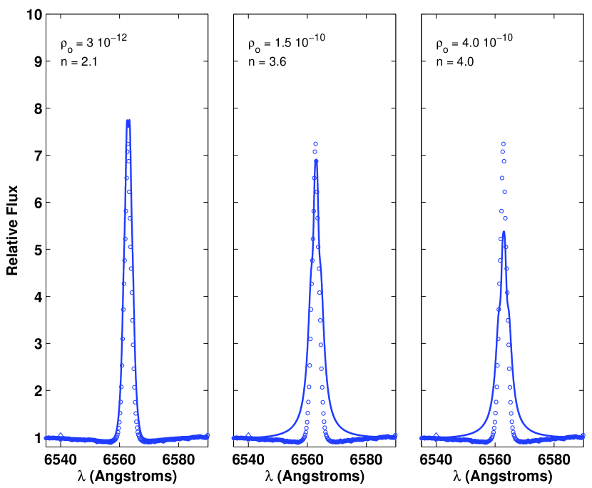
Figure 6: The observed H$\alpha$ line for $\beta$ Psc compared with model predictions for a series of models showing the changes in the profile as $n$ is increased. The model profiles are the solid lines and the circles represent the observation.

We calculated the H$\alpha$ equivalent widths for a subset ($\sim 20$ models) chosen by the best-fit $\chi^{2}$ values, and we considered $\chi^{2}$ values up to $\sim 1.52$. Statistically, the two models corresponding to $\chi^{2}$ values of 0.83, and 0.84 are equally as good while the other models in the subset with larger values of $\chi^{2}$ are poorer fits to the interferometric data. Nevertheless, to be complete we computed profiles for every model in the subset. The equivalent widths for the two models corresponding to the minimum $\chi^{2}$ values had reasonable line shapes compared to the observed profile but the model corresponding to $n=2.2$ had an equivalent width of -25.0 Å  while the model corresponding to $n=2.1$ had an equivalent width of -21.6 Å  which is closer to the value for the observed spectra of -15.3 Å.

Figure 6 shows the H$\alpha$ profile for the best-fit model ($n=2.1$, $\rho_{o}=3.0\times 10^{-12}$ g/cm³) in the left-most panel in terms of interferometric observations and spectroscopy. Models corresponding to other values of $n$ did not produce H$\alpha$ profiles that agreed with observations. Figure 6 shows the behavior of the H$\alpha$ profile with increasing values of $n$. The reader can clearly see that the wings of the line in the middle and right-most panels are too wide, resulting in predicted emission which is too large. These profiles correspond to models with $n=3.6$, $\rho_{o}=1.5\times 10^{-10}$ g/cm³, equivalent width of -30.4 Å, and $n=4.0$, $\rho_{o}=4.0\times 10^{-10}$ g/cm³, equivalent width of -23.4 Å, and have interferometric reduced $\chi^{2}$ values of 1.13, and 1.21, respectively. Models with values of $n<2.1$ had large $\chi^{2}$ values based on the interferometric results, and were eliminated. Figure 7 shows the interferometric observations for our best fit model with $n=2.1$, and $\rho_{o}=3\times 10^{-12}$ g/cm³ for $\beta$ Psc.

Figure 7: The interferometric data and model with $n=2.1$, and $\rho_{o}=3.0\times 10^{-12}$ g/cm³ for $\beta$ Psc. The dashed line represents the central star and the solid line is obtained by taking a Fourier transform of a synthetic image of the preferred model.

4.3 $\upsilon$ Cygnus

$\upsilon$ Cyg has long been recognized as a Be star with strong H$\alpha$ emission (Fleming, 1891; Campbell, 1895). Although several authors have noted that this emission stays relatively constant over periods as long as decades (see, for example, Peters, 1979) others have noted periodic outbursts in H$\alpha$ emission, typical of many Be stars (Ballereau et al., 1995; Neiner, 2005). The interferometric observations for $\upsilon$ Cygnus are from 12 nights between 28 Aug. 2005 and 26 Sept. 2005, and the H$\alpha$ line profile was acquired on 16 Sept. 2005 (see Table 1). We note that we also have observations from 17 Oct. 2005 that confirm the spectroscopic stability of the star.

Neiner (2005) suggested that the outbursts, which occur on periods of $\sim$ years, are the result of multi-periodic, non-radial pulsations. Neiner (2005) derived the stellar parameters for this star by detailed modeling constrained by photometric and spectroscopic data. Three of their models include veiling effects, and gravitational darkening for a range of stellar rotational velocities, 0.80, 0.90, and 0.95 of the critical velocity. (See Neiner (2005) for more detail.) We have chosen to adopt the stellar parameters from their model D which has an intermediate value of the rotational velocity (that is, 0.90 of critical velocity). Also, Neiner (2005) finds a value for the inclination angle of $i\,\sim 27^{o}$. The stellar radius listed in Table 2 corresponds to the equatorial radius given by Neiner (2005). This is a reasonable choice since the star is nearly pole-on. The stellar parameters adopted for $\upsilon$ Cyg are reasonable compared to other values presented in the literature of this spectral type (see for example Cox, 2000).

The procedure for selecting the grid of models to be compared with interferometric observations was obtained by the same selection process as done for the two other stars in this investigation. The final selection of parameters to be searched ranged from $n=1.8$ to $n=4.5$, and $\rho_{o}=1.0\times 10^{-12}$ g/cm³ to $\rho_{o}=4.0\times 10^{-9}$g/cm³, giving a total of 193 models constructed for comparison with interferometric observations. The corresponding $\chi^{2}$ values had a minimum value of 1.14 corresponding to the model with $n=4.0$ and $\rho_{o}=8.0\times 10^{-10}$ g/cm³ and a maximum value of 471 corresponding the model with $n=1.8$ and $\rho_{o}=8.0\times 10^{-12}$ g/cm³. The $\chi^{2}$ values revealed several models that statistically fit the observations equally well. Again, we turn to spectroscopy to remove the degeneracy.

In order to predict H$\alpha$ profiles we adopt $i=30^{\rm o}$ which is consistent with Neiner (2005). We calculate the H$\alpha$ equivalent widths for a subset ($\sim 22$ models) chosen based on the interferometric reduced $\chi^{2}<2$. Statistically, the models with larger values of $\chi^{2}$ are poorer fits to the interferometric data. The equivalent widths for the subset ranged from a minimum of -19.0 Å  to a maximum of -43.1 Å. The observed H$\alpha$ line has an equivalent width of -24.8 Å, and there were three models which had reasonable line shapes and equivalent widths that agreed within $\pm 2$ Å  and had statistically similar interferometric $\chi^{2}$ values. Figure 8 shows the H$\alpha$ profiles corresponding to these models. Table 3 lists the values of $n$, $\rho_{o}$, H$\alpha$ equivalent width, and the reduced $\chi^{2}$ values based on comparisons from interferometry for these 3 models. The models with $n=4.1$ and $n=4.2$ in Figure 8 have predicted profiles that are too narrow and also do not fit the peak of the observed profile. Since the $\chi^{2}$ values are statistically similar, we adopt the model corresponding to $n=4.0$ and $\rho_{o}=8.0\times 10^{-10}$ g/cm³ in Figure 8 as the best-fit. As a further illustration, Figure 9 shows H$\alpha$ profiles corresponding to models with smaller and larger values of $n$ than those given in Table 3. Specifically, these profiles correspond to models with $n=3.6$, $\rho_{o}=3.0\times 10^{-10}$ g/cm³ and $n=4.4$, $\rho_{o}=2.0\times 10^{-9}$ g/cm³ with reduced $\chi^{2}$ values of 1.37, and 1.29, respectively. The shapes of these profiles do not match the observed line. The predicted profile corresponding to $n=3.6$ has too much emission (with an equivalent width of -33.7 Å) and is too wide in the line wings. The predicted profile corresponding to $n=4.4$, has too little emission (with an equivalent width of -20.3 Å) and much of the profile is narrower than the observation. Figure 10 shows a comparison of the interferometric observations and the best-fit model for $\upsilon$ Cyg.

Table 3: Best-Fit Models for $\upsilon$ Cygnus

$n$	$\rho_{o}$	H$\alpha$ Equivalent	$\chi^{2}$
	g/cm3	Width [Å]
4.0	$8.0\times 10^{-10}$	-26.0	1.14
4.1	$1.0\times 10^{-9}$	-24.4	1.16
4.2	$1.5\times 10^{-9}$	-23.7	1.30

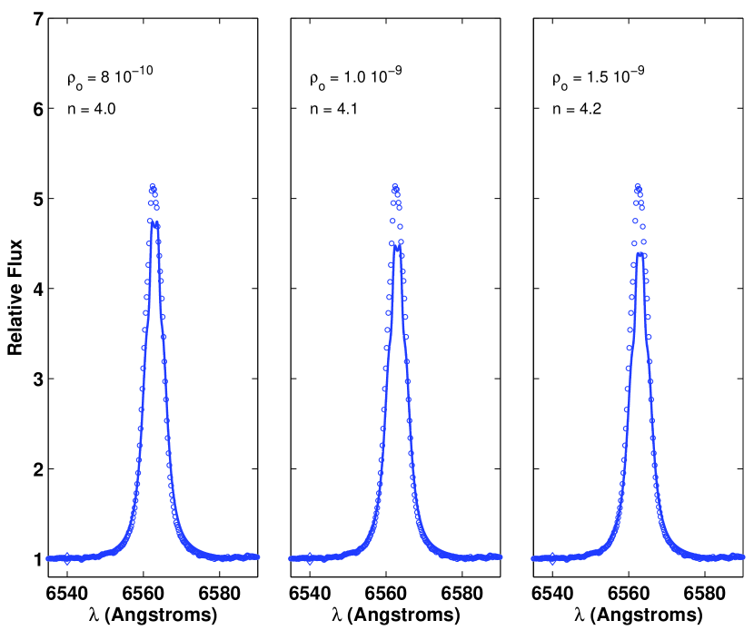
Figure 8: The observed H$\alpha$ line for $\upsilon$ Cyg compared with the best predicted lines from the models which are also in agreement with the interferometric observations. The model profiles are the solid lines and the circles represent the observed line. See Table 3 for the model parameters, H$\alpha$ equivalent widths, and the reduced $\chi^{2}$ values from interferometry corresponding to these models.

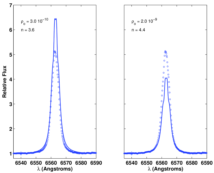
Figure 9: The observed H$\alpha$ lines for $\upsilon$ Cyg compared with the best predicted lines for $n=3.6$ and $n=4.4$. The model profiles are the solid lines and the circles represent the observed line. The model on the left panel has a lower value of $n$ and higher density, resulting in an H$\alpha$ profile which is too large. The model on the right panel has a higher value of $n$ and lower density, resulting in an H$\alpha$ profile which is too small.

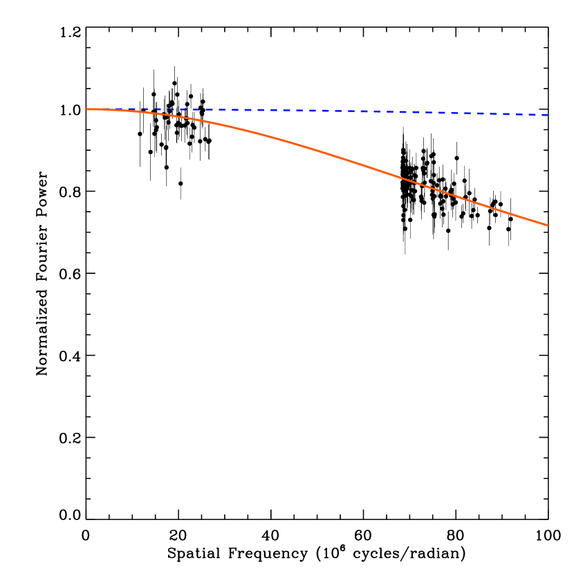
Figure 10: The interferometric data and model with $n=4.0$, and $\rho_{o}=8.0\times 10^{-10}$ g/cm³ for $\upsilon$ Cyg. The dashed line represents the central star and the solid line is obtained by taking a Fourier transform of a synthetic image of the preferred model.

5 Conclusions

In this work, disk density models were obtained for the classical Be stars $\kappa\;$Dra, $\beta\;$Psc, and $\upsilon\;$Cyg by matching the observed interferometric H$\alpha$ visibilities with Fourier transforms of synthetic images produced by theoretical models. It was demonstrated that the additional constraint obtained by the (co-temporal) observed H$\alpha$ line profile was critical to selecting a density model. This was particularly evident in the case of $\kappa$ Dra. We have demonstrated that in the case of these 3 stars, only by additional observational constraints can the degeneracy in the interferometric best-fitting models be removed.

The best fit models to both the interferometric observations and the observed H$\alpha$ line profiles for the three stars are summarized in Table 4. The range of $n$ is consistent with previous determinations based on other diagnostics (such as IR excess see – Waters (1986)). We note that the range of “base” densities, $\rho_{o}$, varies by over two orders of magnitude between the three stars.

Table 4: Summary of Best-Fit Models

Star	$n$	$\rho_{o}$
		g/cm3
$\kappa\;$Dra	4.2	$1.5\times 10^{-10}$
$\beta\;$Psc	2.1	$3.0\times 10^{-12}$
$\upsilon\;$Cyg	4.0	$8.0\times 10^{-10}$

References

- Armstrong et al. (1998) Armstrong, J. T., Mozurkewich, D., Rickard, L. J., Hutter, D. J., Benson, J. A., Bowers, P. F., Elias, N. M. II, Hummel, C. A., Johnston, K. J., Buscher, D. F., and 5 coauthors 1998, ApJ, 496, 550
- Ballereau et al. (1995) Ballereau, D., Chauville, J., & Zorec, J. 1995, A&A, 111, 423
- Barklem & Piskunov (2003) Barklem, P. S., & Piskunov, N. E. 2000 in Model ling of Stellar Atmospheres, IAU Symposium 210, N. E. Piskunov, W. W. Weiss, & D. F. Gray eds., p.E28
- Campbell (1895) Campbell, W. W. 1895, ApJ, 2, 177
- Carciofi & Bjorkman (2006) Carciofi, A. C., & Bjorkman, J. E. 2006, ApJ, 639, 1081
- Chesneau et al. (2005) Chesneau, O., Meilland, A., Rivinius, T., Stee, P., Jankov, S., Domiciano de Souza, A., Graser, U., Herbst, T., Janot-Pacheco, E., Koehler, R., & 5 co-authors. 2005, A&A, 435, 275
- Clarke (1990) Clarke, D. 1990, A&A, 227, 151
- Coté & Waters (1987) Coté, J., & Waters, L. B. F. M. 1987, A&A, 176, 93
- Cox (2000) Cox, A. N.(editor) 2000, Allen’s Astrophysical Quantities, fourth edition, Springer-Verlag, New York
- Coyne & Kruszewski (1969) Coyne, G. V., & Kruszewski, A. 1969, AJ, 74, 528
- Cranmer (2005) Cranmer, S. R. 2005, ApJ, 634, 585
- Dougherty et al. (1991) Dougherty, S. M., Waters, L. B. F. M., Burki, G., Cote, J., Cramer, N., van Kerkwijk, M. H., & Taylor, A. R. 1994, A&A, 290, 609
- Fleming (1891) Fleming, M. 1891, Astronomische Nachrichten, 128, 403
- Gies et al. (2007) Gies, D. R., Bagnuolo, W. G., Jr., Baines, E. K., ten Brummelaar, T. A., Farrington, C. D., Goldfinger, P. J., Grundstrom, E. D., Huang, W., McAlister, H. A., Mérand, A., & 15 coauthors 2007, ApJ, 654, 527
- Hirata (1995) Hirata, R. 1995, PASJ, 47, 195
- Juza et al. (1991) Juza, K., Harmanec, P., Hill, G. M., Tarasov, A. E., & Matthews, J. M. 1991, Bull. Astron. Inst. Czechoslovakia, 42, 39
- Kurucz (1993) Kurucz, R. F. 1993, Kurucz CD-ROM No. 13. Cambridge, Mass: Smithsonian Astrophysical Observatory
- Levenhagen & Leister (2004) Levenhagen, R. S., & Leister, N. V. 2004 ApJ, 127, 1176
- McAlister et al. (2005) McAlister, H. A., Brummelaar, T. A., GiEs, D. R., Huang, W., Bagnuolo, W. G., Jr., Shure, M. A., Sturmann, J., Sturmann, L., Turner, N. H., Taylor, S. F., & 6 co-authors. 2005, ApJ, 628, 439
- Merrill et al. (1925) Merrill, P. W., Humason, M. L., & Burwell, C. G. 1925, ApJ, 61, 389
- Mihalas (1978) Mihalas, D. 1978, Stellar Atmospheres (San Francisco: W. H. Freeman)
- Neiner (2005) Neiner, C., Floquet, M., Hubert, A. M., Frémat, Y., Hirata, R., Masuda, S., Gies, D., Buil, C,; Martayan, C. 2005, A&A, 437, 257 Nuclei, (Mill Valley: Univ. Sci. Books)
- Owocki (2003) Owocki, S. P. 2003, Rotation and Mass Ejection: the Launching of Be-Star Disks in Maeder A., Eenens, P., eds, IAU Symposium 215, Stellar Rotation, 1
- Olson & Kunasz (1987) Olson, G. L., & Kunasz, P. B. 1987, J. Quant. Spectrosc. Radiat. Transfer, 38, 325
- Peters (1979) Peters, G. J. 1979, ApJS, 39, 175
- Porter (1996) Porter, J. M. 1996, MNRAS, 280, 31
- Porter & Rivinus (2003) Porter, J. M., & Rivinius, T. 2003, PASP, 115, 1153
- Saad (2004) Saad, S. M., Kubát, J., Koubský, P., Harmanec, P., Škoda, P., Korčáková, D., Krtička, J., Šlechta, M., Božić, H., Ak, H., Hadrava, P., Votruba, V. 2004, å, 419, 607
- Sigut & Jones (2007) Sigut, T. A. A., & Jones, C. E. 2007 ApJ, 668,481
- Struve (1931) Struve, O. 1931, ApJ, 73, 94
- Townsend et al. (2004) Townsend, R. H. D., Owocki, S. P., & Howarth, I. D. 2004, MNRAS, 350, 189
- Tycner et al. (2003) Tycner, C., Hajian, A. R., Mozurkewich, D., Armstrong, J. T., Benson, J. A., Gilbreath, G. C., Hutter, D. J., Pauls, T. A., & Lester, J. B. 2003, AJ, 125, 3378
- Tycner et al. (2006) Tycner, Christopher, Gilbreath, G. C., Zavala, R. T., Armstrong, J. T., Benson, J. A., Hajian, Arsen R., Hutter, D. J., Jones, C. E., Pauls, T. A., & White, N. M. 2006, AJ, 131, 2710
- Tycner et al. (2008) Tycner, Christopher, Jones, C. E., Sigut, T. A. A. S., Schmitt, H. R., Benson, J. A., Hutter, D. J., & Zavala, R. T. 2008, ApJ, submitted
- van Kerkwijk et al. (1995) van Kerkwijk, M. H., Waters, L. B. F. M., & Marlborough, J. M. 1995, A&A, 300, 259
- Waters (1986) Waters, L. B. F. M. 1986 A&A, 162, 121
- Waters & Coté (1987) Waters, L. B. F. M., Coté, J., & Lamers, H. J. G. L. M. 1987, A&A, 185, 206