Effect of different Dzyaloshinskii-Moriya interactions on entanglement in the Heisenberg XYZ chain

Da-Chuang Li1,2111E-mail: dachuang@ahu.edu.cn, Zhuo-Liang Cao1,2222E-mail:zhuoliangcao@gmail.com (Corresponding Author) 1Department of Physics, Hefei Teachers College, Hefei 230061 P. R. China
2School of Physics & Material Science, Anhui University, Hefei 230039 P. R. China
Abstract

In this paper, we study the thermal entanglement in a two-qubit Heisenberg XYZ system with different Dzyaloshinskii-Moriya (DM) couplings. We show that different DM coupling parameters have different influences on the entanglement and the critical temperature. In addition, we find that when Jisubscript𝐽𝑖J_{i} (i𝑖i-component spin coupling interaction) is the largest spin coupling coefficient, Disubscript𝐷𝑖D_{i} (i𝑖i-component DM interaction) is the most efficient DM control parameter, which can be obtained by adjusting the direction of DM interaction.

Thermal entanglement; Heisenberg XYZ model; DM interaction
pacs:
03.67.Mn, 75.10.Jm, 03.67.Lx

I introduction

Entanglement has been studied intensely in recent years due to its fascinating nonclassical feature and potential applications in quantum information processing 1 . As a simple system, Heisenberg model is an ideal candidate for the generation and the manipulation of entangled states. Many physical systems, such as nuclear spins 2 , quantum dots 3 , superconductor 4 and optical lattices 5 , have been simulated by this model, and the Heisenberg interaction alone can be used for quantum computation by suitable coding 6 . Recently, the Heisenberg models, including Ising model 7 , XY model 8 , XXX model 9 , XXZ model 10 and XYZ model 11 ; 12 , have been intensively studied. Shan et al. investigated the effects of DM interaction, impurity and exchange couplings on entanglement in XY spin chain 16 . Aydiner et al. studied the thermal entanglement of a two-qutrit Ising system with DM interaction 17 , they found that the control of entanglement can be optimized by utilizing competing effects of the magnetic field and the DM interaction. Wang et al. investigated the effects of the DM interaction and intrinsic decoherence on entanglement teleportation in the two-qubit XXX Heisenberg model 18 .

In the above models, the influences of the z-component DM interaction (arising from spin-orbit coupling) and the external magnetic field on the entanglement have been discussed, but the DM coupling interactions along other directions have never been taken into account. Quite recently, we discussed the influences of x-component DM interaction on entanglement in Heisenberg XXZ model 13 and XYZ model 14 . To research further the differences between DM coupling interactions along different directions, in this paper, we generalize the special Heisenberg models to the generalized Heisenberg XYZ models with different DM interactions, and then analyze the different influences of Dxsubscript𝐷π‘₯D_{x} (x-component DM control parameter), Dysubscript𝐷𝑦D_{y} (y-component DM control parameter) and Dzsubscript𝐷𝑧D_{z} (z-component DM control parameter) on the entanglement and the critical temperature. We find that Disubscript𝐷𝑖D_{i} is the most efficient DM control parameter when Jisubscript𝐽𝑖J_{i} is the largest spin coupling coefficient. Thus, according to the relation among Ji​(i=x,y,z)subscript𝐽𝑖𝑖π‘₯𝑦𝑧J_{i}(i=x,y,z), we can know which is the most efficient DM control parameter. In order to provide a detailed analytical and numerical analysis, here we take concurrence as a measure of entanglement 15 . The concurrence C𝐢C ranges from 0 to 1, C=0𝐢0C=0 and C=1𝐢1C=1 indicate the vanishing entanglement and the maximal entanglement respectively. For a mixed state ρ𝜌\rho, the concurrence of the state is C​(ρ)=max⁑{2​λmaxβˆ’βˆ‘i=14Ξ»i,0}𝐢𝜌2subscriptπœ†superscriptsubscript𝑖14subscriptπœ†π‘–0C(\rho)=\max\{2\lambda_{\max}-\sum_{i=1}^{4}\lambda_{i},0\}, where Ξ»i​ssubscriptπœ†π‘–π‘ \lambda_{i}s are the positive square roots of the eigenvalues of the matrix R=ρ​(Οƒy​⨂σy)β€‹Οβˆ—β€‹(Οƒy​⨂σy)π‘…πœŒsuperscriptπœŽπ‘¦tensor-productsuperscriptπœŽπ‘¦superscript𝜌superscriptπœŽπ‘¦tensor-productsuperscriptπœŽπ‘¦R=\rho(\sigma^{y}\bigotimes\sigma^{y})\rho^{*}(\sigma^{y}\bigotimes\sigma^{y}), and the asterisk denotes the complex conjugate.

This paper is organized as follows. In Sec. II, we introduce the Heisenberg XYZ models with different DM interaction parameters, and give the analytical expressions of the concurrences. In Sec. III, we analyze the different influences of different DM control parameters (Dxsubscript𝐷π‘₯D_{x}, Dysubscript𝐷𝑦D_{y} and Dzsubscript𝐷𝑧D_{z}) on the entanglement and the critical temperature. Finally, in Sec. IV a discussion concludes the paper.

II The Heisenberg XYZ models with different DM interaction parameters

II.1 Heisenberg XYZ model with Dxsubscript𝐷π‘₯D_{x}

The Hamiltonian H𝐻H for a two-qubit anisotropic Heisenberg XYZ chain with DM interaction parameter Dxsubscript𝐷π‘₯D_{x} is

H=Jx​σ1x​σ2x+Jy​σ1y​σ2y+Jz​σ1z​σ2z+Dx​(Οƒ1y​σ2zβˆ’Οƒ1z​σ2y),𝐻subscript𝐽π‘₯superscriptsubscript𝜎1π‘₯superscriptsubscript𝜎2π‘₯subscript𝐽𝑦superscriptsubscript𝜎1𝑦superscriptsubscript𝜎2𝑦subscript𝐽𝑧superscriptsubscript𝜎1𝑧superscriptsubscript𝜎2𝑧subscript𝐷π‘₯superscriptsubscript𝜎1𝑦superscriptsubscript𝜎2𝑧superscriptsubscript𝜎1𝑧superscriptsubscript𝜎2𝑦H=J_{x}\sigma_{1}^{x}\sigma_{2}^{x}+J_{y}\sigma_{1}^{y}\sigma_{2}^{y}+J_{z}\sigma_{1}^{z}\sigma_{2}^{z}+D_{x}(\sigma_{1}^{y}\sigma_{2}^{z}-\sigma_{1}^{z}\sigma_{2}^{y}), (1)

where Ji​(i=x,y,z)subscript𝐽𝑖𝑖π‘₯𝑦𝑧J_{i}(i=x,y,z) are the real coupling coefficients, Dxsubscript𝐷π‘₯D_{x} is the x-component DM coupling parameter, and Οƒi​(i=x,y,z)superscriptπœŽπ‘–π‘–π‘₯𝑦𝑧\sigma^{i}(i=x,y,z) are the Pauli matrices. The coupling constants Ji>0subscript𝐽𝑖0J_{i}>0 corresponds to the antiferromagnetic case, and Ji<0subscript𝐽𝑖0J_{i}<0 corresponds to the ferromagnetic case. This model can be reduced to some special Heisenberg models by changing Jisubscript𝐽𝑖J_{i}. Parameters Jisubscript𝐽𝑖J_{i} and Dxsubscript𝐷π‘₯D_{x} are dimensionless.

In the standard basis {|00⟩,|01⟩,|10⟩,|11⟩}ket00ket01ket10ket11\{|00\rangle,|01\rangle,|10\rangle,|11\rangle\}, the Hamiltonian (1) can be rewritten as

H=(Jzi​Dxβˆ’i​DxJxβˆ’Jyβˆ’i​Dxβˆ’JzJx+Jyi​Dxi​DxJx+Jyβˆ’Jzβˆ’i​DxJxβˆ’Jyβˆ’i​Dxi​DxJz).𝐻subscript𝐽𝑧𝑖subscript𝐷π‘₯𝑖subscript𝐷π‘₯subscript𝐽π‘₯subscript𝐽𝑦𝑖subscript𝐷π‘₯subscript𝐽𝑧subscript𝐽π‘₯subscript𝐽𝑦𝑖subscript𝐷π‘₯𝑖subscript𝐷π‘₯subscript𝐽π‘₯subscript𝐽𝑦subscript𝐽𝑧𝑖subscript𝐷π‘₯subscript𝐽π‘₯subscript𝐽𝑦𝑖subscript𝐷π‘₯𝑖subscript𝐷π‘₯subscript𝐽𝑧H=\left(\begin{array}[]{cccc}J_{z}&iD_{x}&-iD_{x}&J_{x}-J_{y}\\ -iD_{x}&-J_{z}&J_{x}+J_{y}&iD_{x}\\ iD_{x}&J_{x}+J_{y}&-J_{z}&-iD_{x}\\ J_{x}-J_{y}&-iD_{x}&iD_{x}&J_{z}\\ \end{array}\right). (2)

By calculating, we can obtain the eigenstates of H𝐻H:

|Ξ¨1⟩=12​(|01⟩+|10⟩),ketsubscriptΞ¨112ket01ket10|\Psi_{1}\rangle=\frac{1}{\sqrt{2}}(|01\rangle+|10\rangle), (3a)
|Ξ¨2⟩=12​(|00⟩+|11⟩),ketsubscriptΞ¨212ket00ket11|\Psi_{2}\rangle=\frac{1}{\sqrt{2}}(|00\rangle+|11\rangle), (3b)
|Ξ¨3⟩=12​(sin⁑θ1​|00βŸ©βˆ’i​cos⁑θ1​|01⟩+i​cos⁑θ1​|10βŸ©βˆ’sin⁑θ1​|11⟩),ketsubscriptΞ¨312subscriptπœƒ1ket00𝑖subscriptπœƒ1ket01𝑖subscriptπœƒ1ket10subscriptπœƒ1ket11|\Psi_{3}\rangle=\frac{1}{\sqrt{2}}(\sin\theta_{1}|00\rangle-i\cos\theta_{1}|01\rangle+i\cos\theta_{1}|10\rangle-\sin\theta_{1}|11\rangle), (3c)
|Ξ¨4⟩=12​(sin⁑θ2​|00⟩+i​cos⁑θ2​|01βŸ©βˆ’i​cos⁑θ2​|10βŸ©βˆ’sin⁑θ2​|11⟩),ketsubscriptΞ¨412subscriptπœƒ2ket00𝑖subscriptπœƒ2ket01𝑖subscriptπœƒ2ket10subscriptπœƒ2ket11|\Psi_{4}\rangle=\frac{1}{\sqrt{2}}(\sin\theta_{2}|00\rangle+i\cos\theta_{2}|01\rangle-i\cos\theta_{2}|10\rangle-\sin\theta_{2}|11\rangle), (3d)

with corresponding eigenvalues:

E1,2=JxΒ±Jyβˆ“Jz,subscript𝐸12minus-or-plusplus-or-minussubscript𝐽π‘₯subscript𝐽𝑦subscript𝐽𝑧E_{1,2}=J_{x}\pm J_{y}\mp J_{z}, (4a)
E3,4=βˆ’JxΒ±w,subscript𝐸34plus-or-minussubscript𝐽π‘₯𝑀E_{3,4}=-J_{x}\pm w, (4b)

where ΞΈ1,2=arctan⁑(2​Dxwβˆ“Jyβˆ“Jz)subscriptπœƒ122subscript𝐷π‘₯minus-or-plus𝑀subscript𝐽𝑦subscript𝐽𝑧\theta_{1,2}=\arctan(\frac{2D_{x}}{w\mp J_{y}\mp J_{z}}), and w=4​Dx2+(Jy+Jz)2𝑀4subscriptsuperscript𝐷2π‘₯superscriptsubscript𝐽𝑦subscript𝐽𝑧2w=\sqrt{4D^{2}_{x}+(J_{y}+J_{z})^{2}}. The system state at thermal equilibrium (thermal state) is ρ​(T)=exp⁑(βˆ’HKB​T)ZπœŒπ‘‡π»subscript𝐾𝐡𝑇𝑍\rho(T)=\frac{\exp(\frac{-H}{K_{B}T})}{Z}, where Z=T​r​[exp⁑(βˆ’HKB​T)]π‘π‘‡π‘Ÿdelimited-[]𝐻subscript𝐾𝐡𝑇Z=Tr[\exp(\frac{-H}{K_{B}T})] is the partition function of the system, H𝐻H is the system Hamiltonian, T𝑇T is the temperature and KBsubscript𝐾𝐡K_{B} is the Boltzmann costant which we take equal to 1 for simplicity. Thus, in the above standard basis, we can get the following analytical expression of the density matrix ρ​(T)πœŒπ‘‡\rho(T):

ρ​(T)=(m1qqβˆ—m2qβˆ—n1n2qqn2n1qβˆ—m2qβˆ—qm1),πœŒπ‘‡subscriptπ‘š1π‘žsuperscriptπ‘žsubscriptπ‘š2superscriptπ‘žsubscript𝑛1subscript𝑛2π‘žπ‘žsubscript𝑛2subscript𝑛1superscriptπ‘žsubscriptπ‘š2superscriptπ‘žπ‘žsubscriptπ‘š1\rho(T)=\left(\begin{array}[]{cccc}m_{1}&q&q^{*}&m_{2}\\ q^{*}&n_{1}&n_{2}&q\\ q&n_{2}&n_{1}&q^{*}\\ m_{2}&q^{*}&q&m_{1}\\ \end{array}\right), (5)

where

m1,2=12​Z​(eβˆ’E2TΒ±eβˆ’E3T​sin2⁑θ1Β±eβˆ’E4T​sin2⁑θ2),subscriptπ‘š1212𝑍plus-or-minussuperscript𝑒subscript𝐸2𝑇superscript𝑒subscript𝐸3𝑇superscript2subscriptπœƒ1superscript𝑒subscript𝐸4𝑇superscript2subscriptπœƒ2\displaystyle m_{1,2}=\frac{1}{2Z}\big{(}e^{-\frac{E_{2}}{T}}\pm e^{-\frac{E_{3}}{T}}\sin^{2}\theta_{1}\pm e^{-\frac{E_{4}}{T}}\sin^{2}\theta_{2}\big{)},
n1,2=12​Z​(eβˆ’E1TΒ±eβˆ’E3T​cos2⁑θ1Β±eβˆ’E4T​cos2⁑θ2),subscript𝑛1212𝑍plus-or-minussuperscript𝑒subscript𝐸1𝑇superscript𝑒subscript𝐸3𝑇superscript2subscriptπœƒ1superscript𝑒subscript𝐸4𝑇superscript2subscriptπœƒ2\displaystyle n_{1,2}=\frac{1}{2Z}\big{(}e^{-\frac{E_{1}}{T}}\pm e^{-\frac{E_{3}}{T}}\cos^{2}\theta_{1}\pm e^{-\frac{E_{4}}{T}}\cos^{2}\theta_{2}\big{)},
q=i2​Z​(eβˆ’E3T​sin⁑θ1​cos⁑θ1βˆ’eβˆ’E4T​sin⁑θ2​cos⁑θ2).π‘žπ‘–2𝑍superscript𝑒subscript𝐸3𝑇subscriptπœƒ1subscriptπœƒ1superscript𝑒subscript𝐸4𝑇subscriptπœƒ2subscriptπœƒ2\displaystyle q=\frac{i}{2Z}\big{(}e^{-\frac{E_{3}}{T}}\sin\theta_{1}\cos\theta_{1}-e^{-\frac{E_{4}}{T}}\sin\theta_{2}\cos\theta_{2}\big{)}.

After straightforward calculations, the positive square roots of the eigenvalues of the matrix R=ρ​(Οƒy​⨂σy)β€‹Οβˆ—β€‹(Οƒy​⨂σy)π‘…πœŒsuperscriptπœŽπ‘¦tensor-productsuperscriptπœŽπ‘¦superscript𝜌superscriptπœŽπ‘¦tensor-productsuperscriptπœŽπ‘¦R=\rho(\sigma^{y}\bigotimes\sigma^{y})\rho^{*}(\sigma^{y}\bigotimes\sigma^{y}) can be expressed as:

Ξ»1,2=1Z​eJxΒ±wT,subscriptπœ†121𝑍superscript𝑒plus-or-minussubscript𝐽π‘₯𝑀𝑇\displaystyle\lambda_{1,2}=\frac{1}{Z}e^{\frac{J_{x}\pm w}{T}}, (6a)
Ξ»3,4=1Z​eβˆ’JxΒ±Jyβˆ“JzT,subscriptπœ†341𝑍superscript𝑒minus-or-plusplus-or-minussubscript𝐽π‘₯subscript𝐽𝑦subscript𝐽𝑧𝑇\displaystyle\lambda_{3,4}=\frac{1}{Z}e^{\frac{-J_{x}\pm J_{y}\mp J_{z}}{T}}, (6b)

where Z=2​eβˆ’JxT​cosh⁑(Jyβˆ’JzT)+2​eJxT​cosh⁑(wT)𝑍2superscript𝑒subscript𝐽π‘₯𝑇subscript𝐽𝑦subscript𝐽𝑧𝑇2superscript𝑒subscript𝐽π‘₯𝑇𝑀𝑇Z=2e^{\frac{-J_{x}}{T}}\cosh(\frac{J_{y}-J_{z}}{T})+2e^{\frac{J_{x}}{T}}\cosh(\frac{w}{T}). Thus, the concurrence of this system can be expressed as 15 :

C={max⁑{|Ξ»1βˆ’Ξ»3|βˆ’Ξ»2βˆ’Ξ»4,0},i​f​Jy>Jz,max⁑{|Ξ»1βˆ’Ξ»4|βˆ’Ξ»2βˆ’Ξ»3,0},i​f​Jyβ©½Jz.𝐢casessubscriptπœ†1subscriptπœ†3subscriptπœ†2subscriptπœ†40𝑖𝑓subscript𝐽𝑦subscript𝐽𝑧subscriptπœ†1subscriptπœ†4subscriptπœ†2subscriptπœ†30𝑖𝑓subscript𝐽𝑦subscript𝐽𝑧\displaystyle C=\left\{\begin{array}[]{l}\max\{|\lambda_{1}-\lambda_{3}|-\lambda_{2}-\lambda_{4},0\},\,\,\,if\,\,\ J_{y}>J_{z},\\ \max\{|\lambda_{1}-\lambda_{4}|-\lambda_{2}-\lambda_{3},0\},\,\,\,if\,\,\ J_{y}\leqslant J_{z}.\\ \end{array}\right. (9)

which is consistent with the results in Ref. 13 for Jx=Jysubscript𝐽π‘₯subscript𝐽𝑦J_{x}=J_{y}.

II.2 Heisenberg XYZ model with Dysubscript𝐷𝑦D_{y}

Here we consider the case of the two-qubit anisotropic Heisenberg XYZ chain with y-component DM parameter Dysubscript𝐷𝑦D_{y}. The Hamiltonian is

Hβ€²=Jx​σ1x​σ2x+Jy​σ1y​σ2y+Jz​σ1z​σ2z+Dy​(Οƒ1z​σ2xβˆ’Οƒ1x​σ2z),superscript𝐻′subscript𝐽π‘₯superscriptsubscript𝜎1π‘₯superscriptsubscript𝜎2π‘₯subscript𝐽𝑦superscriptsubscript𝜎1𝑦superscriptsubscript𝜎2𝑦subscript𝐽𝑧superscriptsubscript𝜎1𝑧superscriptsubscript𝜎2𝑧subscript𝐷𝑦superscriptsubscript𝜎1𝑧superscriptsubscript𝜎2π‘₯superscriptsubscript𝜎1π‘₯superscriptsubscript𝜎2𝑧H^{\prime}=J_{x}\sigma_{1}^{x}\sigma_{2}^{x}+J_{y}\sigma_{1}^{y}\sigma_{2}^{y}+J_{z}\sigma_{1}^{z}\sigma_{2}^{z}+D_{y}(\sigma_{1}^{z}\sigma_{2}^{x}-\sigma_{1}^{x}\sigma_{2}^{z}), (10)

where Dysubscript𝐷𝑦D_{y} is the y-component DM coupling parameter, which is also dimensionless.

In the standard basis {|00⟩,|01⟩,|10⟩,|11⟩}ket00ket01ket10ket11\{|00\rangle,|01\rangle,|10\rangle,|11\rangle\}, the Hamiltonian (8) can be rewritten as

Hβ€²=(JzDyβˆ’DyJxβˆ’JyDyβˆ’JzJx+JyDyβˆ’DyJx+Jyβˆ’Jzβˆ’DyJxβˆ’JyDyβˆ’DyJz).superscript𝐻′subscript𝐽𝑧subscript𝐷𝑦subscript𝐷𝑦subscript𝐽π‘₯subscript𝐽𝑦subscript𝐷𝑦subscript𝐽𝑧subscript𝐽π‘₯subscript𝐽𝑦subscript𝐷𝑦subscript𝐷𝑦subscript𝐽π‘₯subscript𝐽𝑦subscript𝐽𝑧subscript𝐷𝑦subscript𝐽π‘₯subscript𝐽𝑦subscript𝐷𝑦subscript𝐷𝑦subscript𝐽𝑧H^{\prime}=\left(\begin{array}[]{cccc}J_{z}&D_{y}&-D_{y}&J_{x}-J_{y}\\ D_{y}&-J_{z}&J_{x}+J_{y}&D_{y}\\ -D_{y}&J_{x}+J_{y}&-J_{z}&-D_{y}\\ J_{x}-J_{y}&D_{y}&-D_{y}&J_{z}\\ \end{array}\right). (11)

Similarly, by calculating, we can obtain the eigenstates of Hβ€²superscript𝐻′H^{\prime}:

|Ξ¨1β€²βŸ©=12​(|01⟩+|10⟩),ketsuperscriptsubscriptΞ¨1β€²12ket01ket10|\Psi_{1}^{\prime}\rangle=\frac{1}{\sqrt{2}}(|01\rangle+|10\rangle), (12a)
|Ξ¨2β€²βŸ©=12​(|00βŸ©βˆ’|11⟩),ketsuperscriptsubscriptΞ¨2β€²12ket00ket11|\Psi_{2}^{\prime}\rangle=\frac{1}{\sqrt{2}}(|00\rangle-|11\rangle), (12b)
|Ξ¨3β€²βŸ©=12​(sin⁑ϕ1​|00βŸ©βˆ’cos⁑ϕ1​|01⟩+cos⁑ϕ1​|10⟩+sin⁑ϕ1​|11⟩),ketsuperscriptsubscriptΞ¨3β€²12subscriptitalic-Ο•1ket00subscriptitalic-Ο•1ket01subscriptitalic-Ο•1ket10subscriptitalic-Ο•1ket11|\Psi_{3}^{\prime}\rangle=\frac{1}{\sqrt{2}}(\sin\phi_{1}|00\rangle-\cos\phi_{1}|01\rangle+\cos\phi_{1}|10\rangle+\sin\phi_{1}|11\rangle), (12c)
|Ξ¨4β€²βŸ©=12​(sin⁑ϕ2​|00βŸ©βˆ’cos⁑ϕ2​|01⟩+cos⁑ϕ2​|10⟩+sin⁑ϕ2​|11⟩),ketsuperscriptsubscriptΞ¨4β€²12subscriptitalic-Ο•2ket00subscriptitalic-Ο•2ket01subscriptitalic-Ο•2ket10subscriptitalic-Ο•2ket11|\Psi_{4}^{\prime}\rangle=\frac{1}{\sqrt{2}}(\sin\phi_{2}|00\rangle-\cos\phi_{2}|01\rangle+\cos\phi_{2}|10\rangle+\sin\phi_{2}|11\rangle), (12d)

with corresponding eigenvalues:

E1,2β€²=JyΒ±Jxβˆ“Jz,superscriptsubscript𝐸12β€²minus-or-plusplus-or-minussubscript𝐽𝑦subscript𝐽π‘₯subscript𝐽𝑧E_{1,2}^{\prime}=J_{y}\pm J_{x}\mp J_{z}, (13a)
E3,4β€²=βˆ’JyΒ±wβ€²,superscriptsubscript𝐸34β€²plus-or-minussubscript𝐽𝑦superscript𝑀′E_{3,4}^{\prime}=-J_{y}\pm w^{\prime}, (13b)

where Ο•1,2=arctan⁑(2​DyJx+Jzβˆ“wβ€²)subscriptitalic-Ο•122subscript𝐷𝑦minus-or-plussubscript𝐽π‘₯subscript𝐽𝑧superscript𝑀′\phi_{1,2}=\arctan(\frac{2D_{y}}{J_{x}+J_{z}\mp w^{\prime}}), and wβ€²=4​Dy2+(Jx+Jz)2superscript𝑀′4subscriptsuperscript𝐷2𝑦superscriptsubscript𝐽π‘₯subscript𝐽𝑧2w^{\prime}=\sqrt{4D^{2}_{y}+(J_{x}+J_{z})^{2}}. In the above standard basis, the density matrix ρ′​(T)superscriptπœŒβ€²π‘‡\rho^{\prime}(T) has the following form:

ρ′​(T)=(m1β€²βˆ’qβ€²qβ€²m2β€²βˆ’qβ€²n1β€²n2β€²βˆ’qβ€²qβ€²n2β€²n1β€²qβ€²m2β€²βˆ’qβ€²qβ€²m1β€²),superscriptπœŒβ€²π‘‡superscriptsubscriptπ‘š1β€²superscriptπ‘žβ€²superscriptπ‘žβ€²superscriptsubscriptπ‘š2β€²superscriptπ‘žβ€²superscriptsubscript𝑛1β€²superscriptsubscript𝑛2β€²superscriptπ‘žβ€²superscriptπ‘žβ€²superscriptsubscript𝑛2β€²superscriptsubscript𝑛1β€²superscriptπ‘žβ€²superscriptsubscriptπ‘š2β€²superscriptπ‘žβ€²superscriptπ‘žβ€²superscriptsubscriptπ‘š1β€²\rho^{\prime}(T)=\left(\begin{array}[]{cccc}m_{1}^{\prime}&-q^{\prime}&q^{\prime}&m_{2}^{\prime}\\ -q^{\prime}&n_{1}^{\prime}&n_{2}^{\prime}&-q^{\prime}\\ q^{\prime}&n_{2}^{\prime}&n_{1}^{\prime}&q^{\prime}\\ m_{2}^{\prime}&-q^{\prime}&q^{\prime}&m_{1}^{\prime}\\ \end{array}\right), (14)

where

m1,2β€²=12​Z′​(Β±eβˆ’E2β€²T+eβˆ’E3β€²T​sin2⁑ϕ1+eβˆ’E4β€²T​sin2⁑ϕ2),superscriptsubscriptπ‘š12β€²12superscript𝑍′plus-or-minussuperscript𝑒superscriptsubscript𝐸2′𝑇superscript𝑒superscriptsubscript𝐸3′𝑇superscript2subscriptitalic-Ο•1superscript𝑒superscriptsubscript𝐸4′𝑇superscript2subscriptitalic-Ο•2\displaystyle m_{1,2}^{\prime}=\frac{1}{2Z^{\prime}}\big{(}\pm e^{-\frac{E_{2}^{\prime}}{T}}+e^{-\frac{E_{3}^{\prime}}{T}}\sin^{2}\phi_{1}+e^{-\frac{E_{4}^{\prime}}{T}}\sin^{2}\phi_{2}\big{)},
n1,2β€²=12​Z′​(eβˆ’E1β€²TΒ±eβˆ’E3β€²T​cos2⁑ϕ1Β±eβˆ’E4β€²T​cos2⁑ϕ2),superscriptsubscript𝑛12β€²12superscript𝑍′plus-or-minussuperscript𝑒superscriptsubscript𝐸1′𝑇superscript𝑒superscriptsubscript𝐸3′𝑇superscript2subscriptitalic-Ο•1superscript𝑒superscriptsubscript𝐸4′𝑇superscript2subscriptitalic-Ο•2\displaystyle n_{1,2}^{\prime}=\frac{1}{2Z^{\prime}}\big{(}e^{-\frac{E_{1}^{\prime}}{T}}\pm e^{-\frac{E_{3}^{\prime}}{T}}\cos^{2}\phi_{1}\pm e^{-\frac{E_{4}^{\prime}}{T}}\cos^{2}\phi_{2}\big{)},
qβ€²=12​Z′​(eβˆ’E3β€²T​sin⁑ϕ1​cos⁑ϕ1+eβˆ’E4β€²T​sin⁑ϕ2​cos⁑ϕ2).superscriptπ‘žβ€²12superscript𝑍′superscript𝑒superscriptsubscript𝐸3′𝑇subscriptitalic-Ο•1subscriptitalic-Ο•1superscript𝑒superscriptsubscript𝐸4′𝑇subscriptitalic-Ο•2subscriptitalic-Ο•2\displaystyle q^{\prime}=\frac{1}{2Z^{\prime}}\big{(}e^{-\frac{E_{3}^{\prime}}{T}}\sin\phi_{1}\cos\phi_{1}+e^{-\frac{E_{4}^{\prime}}{T}}\sin\phi_{2}\cos\phi_{2}\big{)}.

Then the positive square roots of the eigenvalues of the matrix Rβ€²=ρ′​(Οƒy​⨂σy)β€‹Οβ€²β£βˆ—β€‹(Οƒy​⨂σy)superscript𝑅′superscriptπœŒβ€²superscriptπœŽπ‘¦tensor-productsuperscriptπœŽπ‘¦superscriptπœŒβ€²superscriptπœŽπ‘¦tensor-productsuperscriptπœŽπ‘¦R^{\prime}=\rho^{\prime}(\sigma^{y}\bigotimes\sigma^{y})\rho^{\prime*}(\sigma^{y}\bigotimes\sigma^{y}) can be obtained

Ξ»1,2β€²=1Z′​eβˆ’JyΒ±Jxβˆ“JzT,subscriptsuperscriptπœ†β€²121superscript𝑍′superscript𝑒minus-or-plusplus-or-minussubscript𝐽𝑦subscript𝐽π‘₯subscript𝐽𝑧𝑇\displaystyle\lambda^{\prime}_{1,2}=\frac{1}{Z^{\prime}}e^{\frac{-J_{y}\pm J_{x}\mp J_{z}}{T}}, (15a)
Ξ»3,4β€²=1Z′​eJyΒ±wβ€²T,subscriptsuperscriptπœ†β€²341superscript𝑍′superscript𝑒plus-or-minussubscript𝐽𝑦superscript𝑀′𝑇\displaystyle\lambda^{\prime}_{3,4}=\frac{1}{Z^{\prime}}e^{\frac{J_{y}\pm w^{\prime}}{T}}, (15b)

where Zβ€²=2​eβˆ’JyT​cosh⁑(Jxβˆ’JzT)+2​eJyT​cosh⁑(wβ€²T)superscript𝑍′2superscript𝑒subscript𝐽𝑦𝑇subscript𝐽π‘₯subscript𝐽𝑧𝑇2superscript𝑒subscript𝐽𝑦𝑇superscript𝑀′𝑇Z^{\prime}=2e^{\frac{-J_{y}}{T}}\cosh(\frac{J_{x}-J_{z}}{T})+2e^{\frac{J_{y}}{T}}\cosh(\frac{w^{\prime}}{T}). Thus, the concurrence of this system can be expressed as:

C={max⁑{|Ξ»1β€²βˆ’Ξ»3β€²|βˆ’Ξ»2β€²βˆ’Ξ»4β€²,0},i​f​Jx>Jz,max⁑{|Ξ»2β€²βˆ’Ξ»3β€²|βˆ’Ξ»1β€²βˆ’Ξ»4β€²,0},i​f​Jxβ©½Jz.𝐢casessubscriptsuperscriptπœ†β€²1subscriptsuperscriptπœ†β€²3subscriptsuperscriptπœ†β€²2subscriptsuperscriptπœ†β€²40𝑖𝑓subscript𝐽π‘₯subscript𝐽𝑧subscriptsuperscriptπœ†β€²2subscriptsuperscriptπœ†β€²3subscriptsuperscriptπœ†β€²1subscriptsuperscriptπœ†β€²40𝑖𝑓subscript𝐽π‘₯subscript𝐽𝑧\displaystyle C=\left\{\begin{array}[]{l}\max\{|\lambda^{\prime}_{1}-\lambda^{\prime}_{3}|-\lambda^{\prime}_{2}-\lambda^{\prime}_{4},0\},\,\,\,if\,\,\ J_{x}>J_{z},\\ \max\{|\lambda^{\prime}_{2}-\lambda^{\prime}_{3}|-\lambda^{\prime}_{1}-\lambda^{\prime}_{4},0\},\,\,\,if\,\,\ J_{x}\leqslant J_{z}.\\ \end{array}\right. (18)

II.3 Heisenberg XYZ model with Dzsubscript𝐷𝑧D_{z}

The Hamiltonian Hβ€²β€²superscript𝐻′′H^{\prime\prime} of a two-qubit anisotropic Heisenberg XYZ chain with z-component DM parameter Dzsubscript𝐷𝑧D_{z} is

Hβ€²β€²=Jx​σ1x​σ2x+Jy​σ1y​σ2y+Jz​σ1z​σ2z+Dz​(Οƒ1x​σ2yβˆ’Οƒ1y​σ2x),superscript𝐻′′subscript𝐽π‘₯superscriptsubscript𝜎1π‘₯superscriptsubscript𝜎2π‘₯subscript𝐽𝑦superscriptsubscript𝜎1𝑦superscriptsubscript𝜎2𝑦subscript𝐽𝑧superscriptsubscript𝜎1𝑧superscriptsubscript𝜎2𝑧subscript𝐷𝑧superscriptsubscript𝜎1π‘₯superscriptsubscript𝜎2𝑦superscriptsubscript𝜎1𝑦superscriptsubscript𝜎2π‘₯H^{\prime\prime}=J_{x}\sigma_{1}^{x}\sigma_{2}^{x}+J_{y}\sigma_{1}^{y}\sigma_{2}^{y}+J_{z}\sigma_{1}^{z}\sigma_{2}^{z}+D_{z}(\sigma_{1}^{x}\sigma_{2}^{y}-\sigma_{1}^{y}\sigma_{2}^{x}), (19)

where Dzsubscript𝐷𝑧D_{z} is the z-component DM coupling parameter, which is also dimensionless.

Using the similar process, we can get the eigenstates of Hβ€²β€²superscript𝐻′′H^{\prime\prime}:

|Ξ¨1,2β€²β€²βŸ©=12​(|00⟩±|11⟩),ketsuperscriptsubscriptΞ¨12β€²β€²12plus-or-minusket00ket11|\Psi_{1,2}^{\prime\prime}\rangle=\frac{1}{\sqrt{2}}(|00\rangle\pm|11\rangle), (20a)
|Ξ¨3,4β€²β€²βŸ©=12​(|01βŸ©Β±Ο‡β€‹|10⟩),ketsuperscriptsubscriptΞ¨34β€²β€²12plus-or-minusket01πœ’ket10|\Psi_{3,4}^{\prime\prime}\rangle=\frac{1}{\sqrt{2}}(|01\rangle\pm\chi|10\rangle), (20b)

with corresponding eigenvalues:

E1,2β€²β€²=JzΒ±Jxβˆ“Jy,superscriptsubscript𝐸12β€²β€²minus-or-plusplus-or-minussubscript𝐽𝑧subscript𝐽π‘₯subscript𝐽𝑦E_{1,2}^{\prime\prime}=J_{z}\pm J_{x}\mp J_{y}, (21a)
E3,4β€²β€²=βˆ’JzΒ±wβ€²β€²,superscriptsubscript𝐸34β€²β€²plus-or-minussubscript𝐽𝑧superscript𝑀′′E_{3,4}^{\prime\prime}=-J_{z}\pm w^{\prime\prime}, (21b)

where Ο‡=Jx+Jyβˆ’2​i​Dz4​Dz2+(Jx+Jy)2πœ’subscript𝐽π‘₯subscript𝐽𝑦2𝑖subscript𝐷𝑧4subscriptsuperscript𝐷2𝑧superscriptsubscript𝐽π‘₯subscript𝐽𝑦2\chi=\frac{J_{x}+J_{y}-2iD_{z}}{\sqrt{4D^{2}_{z}+(J_{x}+J_{y})^{2}}}, and wβ€²β€²=4​Dz2+(Jx+Jy)2superscript𝑀′′4subscriptsuperscript𝐷2𝑧superscriptsubscript𝐽π‘₯subscript𝐽𝑦2w^{\prime\prime}=\sqrt{4D^{2}_{z}+(J_{x}+J_{y})^{2}}. Similarly, we can get the analytical expressions of ρ​(T)β€²β€²πœŒsuperscript𝑇′′\rho(T)^{\prime\prime} and Rβ€²β€²superscript𝑅′′R^{\prime\prime}, but we do not list them because of the complexity. After straightforward calculations, the positive square roots of the eigenvalues of Rβ€²β€²=ρ′′​(Οƒy​⨂σy)β€‹Οβ€²β€²β£βˆ—β€‹(Οƒy​⨂σy)superscript𝑅′′superscriptπœŒβ€²β€²superscriptπœŽπ‘¦tensor-productsuperscriptπœŽπ‘¦superscriptπœŒβ€²β€²superscriptπœŽπ‘¦tensor-productsuperscriptπœŽπ‘¦R^{\prime\prime}=\rho^{\prime\prime}(\sigma^{y}\bigotimes\sigma^{y})\rho^{\prime\prime*}(\sigma^{y}\bigotimes\sigma^{y}) can be expressed as:

Ξ»1,2β€²β€²=1Z′′​eJzΒ±wβ€²β€²T,superscriptsubscriptπœ†12β€²β€²1superscript𝑍′′superscript𝑒plus-or-minussubscript𝐽𝑧superscript𝑀′′𝑇\displaystyle\lambda_{1,2}^{\prime\prime}=\frac{1}{Z^{\prime\prime}}e^{\frac{J_{z}\pm w^{\prime\prime}}{T}}, (22a)
Ξ»3,4β€²β€²=1Z′′​eβˆ’JzΒ±Jxβˆ“JyT,superscriptsubscriptπœ†34β€²β€²1superscript𝑍′′superscript𝑒minus-or-plusplus-or-minussubscript𝐽𝑧subscript𝐽π‘₯subscript𝐽𝑦𝑇\displaystyle\lambda_{3,4}^{\prime\prime}=\frac{1}{Z^{\prime\prime}}e^{\frac{-J_{z}\pm J_{x}\mp J_{y}}{T}}, (22b)

with Zβ€²β€²=2​eβˆ’JzT​cosh⁑(Jxβˆ’JyT)+2​eJzT​cosh⁑(wβ€²β€²T)superscript𝑍′′2superscript𝑒subscript𝐽𝑧𝑇subscript𝐽π‘₯subscript𝐽𝑦𝑇2superscript𝑒subscript𝐽𝑧𝑇superscript𝑀′′𝑇Z^{\prime\prime}=2e^{\frac{-J_{z}}{T}}\cosh(\frac{J_{x}-J_{y}}{T})+2e^{\frac{J_{z}}{T}}\cosh(\frac{w^{\prime\prime}}{T}). Thus, the concurrence of this system can be written as:

C={max⁑{|Ξ»1β€²β€²βˆ’Ξ»3β€²β€²|βˆ’Ξ»2β€²β€²βˆ’Ξ»4β€²β€²,0},i​f​Jx>Jy,max⁑{|Ξ»1β€²β€²βˆ’Ξ»4β€²β€²|βˆ’Ξ»2β€²β€²βˆ’Ξ»3β€²β€²,0},i​f​Jxβ©½Jy.𝐢casessuperscriptsubscriptπœ†1β€²β€²superscriptsubscriptπœ†3β€²β€²superscriptsubscriptπœ†2β€²β€²superscriptsubscriptπœ†4β€²β€²0𝑖𝑓subscript𝐽π‘₯subscript𝐽𝑦superscriptsubscriptπœ†1β€²β€²superscriptsubscriptπœ†4β€²β€²superscriptsubscriptπœ†2β€²β€²superscriptsubscriptπœ†3β€²β€²0𝑖𝑓subscript𝐽π‘₯subscript𝐽𝑦\displaystyle C=\left\{\begin{array}[]{l}\max\{|\lambda_{1}^{\prime\prime}-\lambda_{3}^{\prime\prime}|-\lambda_{2}^{\prime\prime}-\lambda_{4}^{\prime\prime},0\},\,\,\,if\,\,\ J_{x}>J_{y},\\ \max\{|\lambda_{1}^{\prime\prime}-\lambda_{4}^{\prime\prime}|-\lambda_{2}^{\prime\prime}-\lambda_{3}^{\prime\prime},0\},\,\,\,if\,\,\ J_{x}\leqslant J_{y}.\\ \end{array}\right. (25)

which is also consistent with the results in Ref. 13 when Jx=Jysubscript𝐽π‘₯subscript𝐽𝑦J_{x}=J_{y}.

Refer to caption
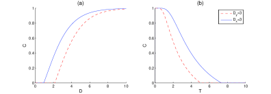
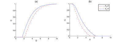
Figure 1: (Color online) (a) The concurrence is plotted versus Dxsubscript𝐷π‘₯D_{x} (blue solid line) and Dysubscript𝐷𝑦D_{y} (red dashed line) for T=3𝑇3T=3. (b) The concurrence is plotted as a function of the temperature T𝑇T for Dx=3subscript𝐷π‘₯3D_{x}=3 (blue solid line) and Dy=3subscript𝐷𝑦3D_{y}=3 (red dashed line). Here the coupling constants Jx=0.2subscript𝐽π‘₯0.2J_{x}=0.2, Jy=βˆ’1subscript𝐽𝑦1J_{y}=-1 and Jz=βˆ’0.5subscript𝐽𝑧0.5J_{z}=-0.5.
Refer to caption
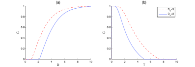
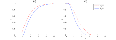
Figure 2: (Color online) (a) The concurrence is plotted versus Dxsubscript𝐷π‘₯D_{x} (blue solid line) and Dysubscript𝐷𝑦D_{y} (red dashed line) for T=3𝑇3T=3. (b) The concurrence is plotted as a function of the temperature T𝑇T for Dx=3subscript𝐷π‘₯3D_{x}=3 (blue solid line) and Dy=3subscript𝐷𝑦3D_{y}=3 (red dashed line). Here the coupling constants Jx=βˆ’1subscript𝐽π‘₯1J_{x}=-1, Jy=0.2subscript𝐽𝑦0.2J_{y}=0.2 and Jz=βˆ’0.5subscript𝐽𝑧0.5J_{z}=-0.5.

From Eqs. (7), (14) and (19), one can see that when Jx=Jysubscript𝐽π‘₯subscript𝐽𝑦J_{x}=J_{y}, there is the same entanglement for Dx=Dysubscript𝐷π‘₯subscript𝐷𝑦D_{x}=D_{y}; when Jy=Jzsubscript𝐽𝑦subscript𝐽𝑧J_{y}=J_{z}, there is the same entanglement for Dy=Dzsubscript𝐷𝑦subscript𝐷𝑧D_{y}=D_{z}; and when Jx=Jzsubscript𝐽π‘₯subscript𝐽𝑧J_{x}=J_{z}, there is the same entanglement for Dx=Dzsubscript𝐷π‘₯subscript𝐷𝑧D_{x}=D_{z}. So when Jx=Jy=Jzsubscript𝐽π‘₯subscript𝐽𝑦subscript𝐽𝑧J_{x}=J_{y}=J_{z}, there is also the same entanglement for the same values of DM interaction parameters (Dxsubscript𝐷π‘₯D_{x}, Dysubscript𝐷𝑦D_{y} and Dzsubscript𝐷𝑧D_{z})

III The comparison between the different DM control parameters in Heisenberg XYZ model

III.1 The comparison between Dxsubscript𝐷π‘₯D_{x} and Dysubscript𝐷𝑦D_{y}

In Heisenberg XYZ model, we has analyzed all kinds of spin coupling coefficients satisfying Jx>Jysubscript𝐽π‘₯subscript𝐽𝑦J_{x}>J_{y}. For simplicity, here we choose one set of spin coupling coefficients satisfying Jx>Jysubscript𝐽π‘₯subscript𝐽𝑦J_{x}>J_{y}, and plot Fig. 1 to demonstrate the properties of different DM parameters. In Fig. 1(a), we find the entanglement increases with the increase of DM coupling parameter. Furthermore, the critical value of Dxsubscript𝐷π‘₯D_{x} is smaller than Dysubscript𝐷𝑦D_{y}, and Dxsubscript𝐷π‘₯D_{x} has more entanglement for Dx=Dysubscript𝐷π‘₯subscript𝐷𝑦D_{x}=D_{y}. In Fig. 1(b), we find that increasing temperature will decrease the entanglement, and Dxsubscript𝐷π‘₯D_{x} has a higher critical temperature than the same Dysubscript𝐷𝑦D_{y}, so that the entanglement can exist at higher temperatures for Dxsubscript𝐷π‘₯D_{x}.

Similarly, we has analyzed various spin coupling coefficients satisfying Jx<Jysubscript𝐽π‘₯subscript𝐽𝑦J_{x}<J_{y}. For simplicity, we choose one set of coupling coefficients satisfying Jx<Jysubscript𝐽π‘₯subscript𝐽𝑦J_{x}<J_{y}, and plot Fig. 2 to demonstrate the properties of different DM parameters. In Fig. 2(a), it is shown that increasing the DM coupling parameter can enhance the entanglement. Besides, for a certain temperature, the critical value of Dysubscript𝐷𝑦D_{y} is smaller than Dxsubscript𝐷π‘₯D_{x}, and Dysubscript𝐷𝑦D_{y} has more entanglement for Dx=Dysubscript𝐷π‘₯subscript𝐷𝑦D_{x}=D_{y}. In Fig. 2(b), it is easy to see that Dysubscript𝐷𝑦D_{y} has a higher critical temperature than the same Dxsubscript𝐷π‘₯D_{x}, so that the entanglement can exist at higher temperatures for Dysubscript𝐷𝑦D_{y}.

Thus, the x-component parameter Dxsubscript𝐷π‘₯D_{x} has a smaller critical value, higher critical temperature and more entanglement than the same y-component parameter Dysubscript𝐷𝑦D_{y} for Jx>Jysubscript𝐽π‘₯subscript𝐽𝑦J_{x}>J_{y}, and Dysubscript𝐷𝑦D_{y} has a smaller critical value, higher critical temperature and more entanglement than the same Dxsubscript𝐷π‘₯D_{x} for Jx<Jysubscript𝐽π‘₯subscript𝐽𝑦J_{x}<J_{y}.

III.2 The comparison between Dysubscript𝐷𝑦D_{y} and Dzsubscript𝐷𝑧D_{z}

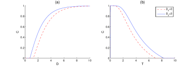
Similarly, for Jy>Jzsubscript𝐽𝑦subscript𝐽𝑧J_{y}>J_{z} case, Fig. 3 is plotted to show the properties of different DM parameters in Heisenberg XYZ model. In Fig. 3(a), we can see that the y-component parameter Dysubscript𝐷𝑦D_{y} has a smaller critical value, and more entanglement for Dy=Dzsubscript𝐷𝑦subscript𝐷𝑧D_{y}=D_{z}. In Fig. 3(b), we can see that Dysubscript𝐷𝑦D_{y} has a higher critical temperature than the same Dzsubscript𝐷𝑧D_{z}, so that the entanglement can exist at higher temperatures for Dysubscript𝐷𝑦D_{y}.

Refer to caption
Figure 3: (Color online) (a) The concurrence is plotted versus Dysubscript𝐷𝑦D_{y} (blue solid line) and Dzsubscript𝐷𝑧D_{z} (red dashed line) for T=3𝑇3T=3. (b) The concurrence is plotted as a function of the temperature T𝑇T for Dy=3subscript𝐷𝑦3D_{y}=3 (blue solid line) and Dz=3subscript𝐷𝑧3D_{z}=3 (red dashed line). Here the coupling constants Jx=βˆ’0.5subscript𝐽π‘₯0.5J_{x}=-0.5, Jy=1subscript𝐽𝑦1J_{y}=1 and Jz=0.2subscript𝐽𝑧0.2J_{z}=0.2.
Refer to caption
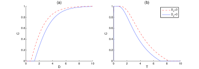
Figure 4: (Color online) (a) The concurrence is plotted versus Dysubscript𝐷𝑦D_{y} (blue solid line) and Dzsubscript𝐷𝑧D_{z} (red dashed line) for T=3𝑇3T=3. (b) The concurrence is plotted as a function of the temperature T𝑇T for Dy=3subscript𝐷𝑦3D_{y}=3 (blue solid line) and Dz=3subscript𝐷𝑧3D_{z}=3 (red dashed line). Here the coupling constants Jx=βˆ’0.5subscript𝐽π‘₯0.5J_{x}=-0.5, Jy=0.2subscript𝐽𝑦0.2J_{y}=0.2 and Jz=1subscript𝐽𝑧1J_{z}=1.

Contrarily, for Jy<Jzsubscript𝐽𝑦subscript𝐽𝑧J_{y}<J_{z} case, the concurrence versus different parameters is shown in Fig. 4. In Fig. 4(a), it is easy to see that the z-component parameter Dzsubscript𝐷𝑧D_{z} has a smaller critical value, and more entanglement for Dy=Dzsubscript𝐷𝑦subscript𝐷𝑧D_{y}=D_{z}. In Fig. 4(b), it is easy to see that Dzsubscript𝐷𝑧D_{z} has a higher critical temperature than the same Dysubscript𝐷𝑦D_{y}, so that the entanglement can also exist at higher temperatures for Dzsubscript𝐷𝑧D_{z}.

Thus, the y-component parameter Dysubscript𝐷𝑦D_{y} has a smaller critical value, higher critical temperature and more entanglement than the same z-component parameter Dzsubscript𝐷𝑧D_{z} for Jy>Jzsubscript𝐽𝑦subscript𝐽𝑧J_{y}>J_{z}, and Dzsubscript𝐷𝑧D_{z} has a smaller critical value, higher critical temperature and more entanglement than the same Dysubscript𝐷𝑦D_{y} for Jy<Jzsubscript𝐽𝑦subscript𝐽𝑧J_{y}<J_{z}.

III.3 The comparison between Dxsubscript𝐷π‘₯D_{x} and Dzsubscript𝐷𝑧D_{z}

Here, for Jx>Jzsubscript𝐽π‘₯subscript𝐽𝑧J_{x}>J_{z} case, we plot Fig. 5 to illustrate the properties of different DM parameters in Heisenberg XYZ model. In Fig. 5(a), Dxsubscript𝐷π‘₯D_{x} has a smaller critical value and more entanglement for Dx=Dzsubscript𝐷π‘₯subscript𝐷𝑧D_{x}=D_{z}. In Fig. 5(b), Dxsubscript𝐷π‘₯D_{x} has a higher critical temperature than the same Dzsubscript𝐷𝑧D_{z}, so that the entanglement can exist at higher temperatures for Dxsubscript𝐷π‘₯D_{x}.

For Jx<Jzsubscript𝐽π‘₯subscript𝐽𝑧J_{x}<J_{z} case, we plot Fig. 6 to illustrate the properties of different DM parameters. In Fig. 6(a), for a certain temperature, Dzsubscript𝐷𝑧D_{z} has a smaller critical value and more entanglement for Dx=Dzsubscript𝐷π‘₯subscript𝐷𝑧D_{x}=D_{z}. In Fig. 6(b), Dzsubscript𝐷𝑧D_{z} has a higher critical temperature than the same Dxsubscript𝐷π‘₯D_{x}, so that the entanglement can also exist at higher temperatures for Dzsubscript𝐷𝑧D_{z}.

Thus, the x-component parameter Dxsubscript𝐷π‘₯D_{x} has a smaller critical value, higher critical temperature and more entanglement than the same z-component parameter Dzsubscript𝐷𝑧D_{z} for Jx>Jzsubscript𝐽π‘₯subscript𝐽𝑧J_{x}>J_{z}, and Dzsubscript𝐷𝑧D_{z} has a smaller critical value, higher critical temperature and more entanglement than the same Dxsubscript𝐷π‘₯D_{x} for Jx<Jzsubscript𝐽π‘₯subscript𝐽𝑧J_{x}<J_{z}.

The above results indicate that when Jisubscript𝐽𝑖J_{i} is the largest spin coupling coefficient, the i-component DM control parameter Disubscript𝐷𝑖D_{i} has the smallest critical value, the highest critical temperature and the most entanglement. So according to the relation among spin coupling coefficients, we can know which is the most efficient DM control parameter.
Refer to caption
Figure 5: (Color online) (a) The concurrence is plotted versus Dxsubscript𝐷π‘₯D_{x} (blue solid line) and Dzsubscript𝐷𝑧D_{z} (red dashed line) for T=3𝑇3T=3. (b) The concurrence is plotted as a function of the temperature T𝑇T for Dx=3subscript𝐷π‘₯3D_{x}=3 (blue solid line) and Dz=3subscript𝐷𝑧3D_{z}=3 (red dashed line). Here the coupling constants Jx=βˆ’0.2subscript𝐽π‘₯0.2J_{x}=-0.2, Jy=0.3subscript𝐽𝑦0.3J_{y}=0.3 and Jz=βˆ’1subscript𝐽𝑧1J_{z}=-1.
Refer to caption
Figure 6: (Color online) (a) The concurrence is plotted versus Dxsubscript𝐷π‘₯D_{x} (blue solid line) and Dzsubscript𝐷𝑧D_{z} (red dashed line) for T=3𝑇3T=3. (b) The concurrence is plotted as a function of the temperature T𝑇T for Dx=3subscript𝐷π‘₯3D_{x}=3 (blue solid line) and Dz=3subscript𝐷𝑧3D_{z}=3 (red dashed line). Here the coupling constants Jx=βˆ’1subscript𝐽π‘₯1J_{x}=-1, Jy=0.3subscript𝐽𝑦0.3J_{y}=0.3 and Jz=βˆ’0.2subscript𝐽𝑧0.2J_{z}=-0.2.

IV Discussion

We have investigated the thermal entanglement in a two-qubit Heisenberg XYZ system with different Dzyaloshinskii-Moriya (DM) couplings. We find that different DM interaction parameters (Dxsubscript𝐷π‘₯D_{x}, Dysubscript𝐷𝑦D_{y} and Dzsubscript𝐷𝑧D_{z}) have different influences on the entanglement and the critical temperature. When Ji​(i=x,y,z)subscript𝐽𝑖𝑖π‘₯𝑦𝑧J_{i}(i=x,y,z) is the largest spin coupling coefficient, the i𝑖i-component DM interaction Di​(i=x,y,z)subscript𝐷𝑖𝑖π‘₯𝑦𝑧D_{i}(i=x,y,z) has the smallest critical value, the highest critical temperature and the most entanglement. In addition, when Jx=Jy=Jzsubscript𝐽π‘₯subscript𝐽𝑦subscript𝐽𝑧J_{x}=J_{y}=J_{z}, there is the same entanglement for the same values of DM interaction parameters (Dxsubscript𝐷π‘₯D_{x}, Dysubscript𝐷𝑦D_{y} and Dzsubscript𝐷𝑧D_{z}). Thus, according to the relation among spin coupling coefficients (Jxsubscript𝐽π‘₯J_{x}, Jysubscript𝐽𝑦J_{y} and Jzsubscript𝐽𝑧J_{z}), the most efficient DM control parameter can be obtained by adjusting the direction of DM interaction.

Acknowledgements.
This work is supported by National Natural Science Foundation of China (NSFC) under Grant Nos: 60678022 and 10704001, the Specialized Research Fund for the Doctoral Program of Higher Education under Grant No. 20060357008, Anhui Provincial Natural Science Foundation under Grant No. 070412060, and the Key Program of the Education Department of Anhui Province under Grant No. KJ2008A28ZC.

References

  • (1) Phys. World 11, 33 (1998), special issue on quantum information; C. H. Bennett and S. J. Wiesner, Phys. Rev. Lett. 69, 2881 (1992); C. H. Bennett et al., ibid. 70, 1895 (1993); A. K. Ekert, ibid. 67, 661 (1991); M. Murao et al., Phys. Rev. A 59, 156 (1999).
  • (2) B. E. Kane, Nature (London) 393, 133 (1998).
  • (3) D. Loss and D. P. DiVincenzo, Phys. Rev. A 57, 120 (1998); G. Burkard, D. Loss, and D. P. DiVincenzo, Phys. Rev. B 59, 2070 (1999); B. Trauzettel et al., Nature Phys. 3 192 (2007).
  • (4) T. Senthil et al., Phys. Rev. B 60 4245 (1999); M. Nishiyama et al., Phys. Rev. Lett. 98 047002 (2007).
  • (5) A. SΓΈrensen and K. MΓΈlmer, Phys. Rev. Lett. 83, 2274 (1999).
  • (6) D. A. Lidar, D. Bacon, and K. B. Whaley, Phys. Rev. Lett. 82, 4556 (1999); D. P. DiVincenzo et al., Nature (London) 408, 339 (2000); L. F. Santos, Phys. Rev. A 67, 062306 (2003).
  • (7) D. Gunlycke et al., Phys. Rev. A 64, 042302 (2001); Z. Yang et al., Phys. Rev. Lett. 100, 067203 (2008).
  • (8) G. L. Kamta and Anthony F. Starace, Phys. Rev. Lett. 88, 107901 (2002); X. G. Wang, Phys. Rev. A 66, 034302 (2002); Y. Sun et al., Phys. Rev. A 68, 044301 (2003); Z. C. Kao et al., Phys. Rev. A 72, 062302 (2005); S. L. Zhu, Phys. Rev. Lett. 96, 077206 (2006).
  • (9) M. Asoudeh and V. Karimipour, Phys. Rev. A 71, 022308 (2005); G. F. Zhang, Phys. Rev. A 75, 034304 (2007).
  • (10) G. F. Zhang and S. S. Li, Phys. Rev. A 72, 034302 (2005); Y. Zhou et al., Phys. Rev. A 75, 062304 (2007); M. Kargarian et al., Phys. Rev. A 77, 032346 (2008).
  • (11) D. C. Li and Z. L. Cao, Optics Communications, in press; L. Zhou et al., Phys. Rev. A 68, 024301 (2003); G. H. Yang et al., e-print arXiv:quant-ph/0602051.
  • (12) F. Kheirandish et al., Phys. Rev. A 77, 042309 (2008); Z. N. Gurkan and O. K. Pashaev, e-print arXiv:quant-ph/0705.0679 and arXiv:quant-ph/0804.0710.
  • (13) Chuan-Jia Shan et al., Chin. Phys. Lett. 25, 817 (2008).
  • (14) C. AkyΓΌz, E. Aydiner, and Γ–. E. MΓΌstecaplioΗ§lu, Optics Communications 281, 5271 (2008).
  • (15) Liang Qiu, An Min Wang, and Xiao Qiang Su, Physica A 387, 6686 (2008).
  • (16) D. C. Li, X. P. Wang, and Z. L. Cao, J. Phys. Condens. Matter 20 325229 (2008).
  • (17) D. C. Li and Z. L. Cao, Eur. Phys. J. D 50, 207 (2008).
  • (18) S. Hill and W. K. Wootters, Phys. Rev. Lett. 78, 5022 (1997); W. K. Wootters, Phys. Rev. Lett. 80, 2245 (1998).