Dynamic treatment of vibrational energy relaxation
in a heterogeneous and fluctuating environment

Abstract

A computational approach to describe the energy relaxation of a high-frequency vibrational mode in a fluctuating heterogeneous environment is outlined. Extending previous work [H. Fujisaki, Y. Zhang, and J.E. Straub, J. Chem. Phys. 124, 144910 (2006)], second-order time-dependent perturbation theory is employed which includes the fluctuations of the parameters in the Hamiltonian within the vibrational adiabatic approximation. This means that the time-dependent vibrational frequencies along an MD trajectory are obtained via a partial geometry optimization of the solute with fixed solvent and a subsequent normal mode calculation. Adopting the amide I mode of N-methylacetamide in heavy water as a test problem, it is shown that the inclusion of dynamic fluctuations may significantly change the vibrational energy relaxation. In particular, it is found that relaxation occurs in two phases, because for short times ($\lesssim$ 200 fs) the spectral density appears continuous due to the frequency-time uncertainty relation, while at longer times the discrete nature of the bath becomes apparent. Considering the excellent agreement between theory and experiment, it is speculated if this behavior can explain the experimentally obtained biphasic relaxation the amide I mode of N-methylacetamide.

I Introduction

Vibrational energy relaxation (VER) is ubiquitous in chemistry and physics. When a chemical reaction or conformational change occurs, some vibrational modes may be excited or de-excited, resulting in nonequilibrium phenomena of VER (for example, see Ref. Agarwal, for the possible role of VER in enzyme reactions). It is usually assumed that VER is much faster than chemical reactions or conformational changes,Steinfeldbook but this is not always the case.LW97 ; GW04 Recent progress in time-resolved spectroscopyMillerReview ; MK97 ; HLH98 ; ZAH01 ; Tokmakoff06 ; FayerReview ; DRID00 ; NNT05 ; Hammreview as well as numerous theoretical formulations Oxtoby ; KTF94 ; Straub ; WWH92 ; Henry ; Straub2 ; NS03 ; Moritsugu2000 ; Nagaoka ; Okazaki ; Geva ; FBS05 ; Leitner05 ; DJBK07 ; Skinner ; Hynes ; Sibert ; Marx04 ; FZS06 ; FS07 ; FYHS07 ; FYHSS08 have been trying to unravel the molecular origin of VER.

To define the problem, we consider the case of the photoinduced $n=1\!\rightarrow\!0$ VER of a high-frequency ($\approx$ 1000$-$2000 cm^-1) vibrational mode in a polyatomic molecule. We partition the total Hamiltonian $H$ as

$$H=H_{S}+H_{B}+H_{SB},$$ (1)

where the system Hamiltonian $H_{S}$ describes the high-frequency mode $\omega_{S}$, the bath Hamiltonian $H_{B}$ comprises all remaining vibrational modes $\omega_{\alpha}$ of the molecule, and $H_{SB}$ accounts for the coupling between the system and bath. The dynamics of the total system is described by the Liouville equation

$${\rm i}\hbar\frac{\partial\rho(t)}{\partial t}=[H,\rho(t)]$$ (2)

with $\rho(t)$ being the density operator for the system and bath. Employing fully quantum-mechanical formulations, various quantum-classical approaches or quasiclassical methods, a number of groups have described VER by calculating the time evolution of the total system. While this strategy is formally exact, it is also quite time-consuming and therefore limited to small molecules or model systems. Thus, various reduced density-matrix formulations for the system part in Eq. (2) have been pursued in the fields of quantum optics, condensed matter physics, and physical chemistry.Weiss ; Breuer ; Nitzan

Considering VER, it is often the case that the coupling $V=H_{SB}-\langle H_{SB}\rangle_{B}$ (where $\langle...\rangle_{B}$ denotes the bath average) is small enough to be described by low-order time-dependent perturbation theory. Assuming, for simplicity, that the VER is dominated by cubic coupling $C_{S\alpha\beta}$ between the system mode $q_{S}$ and two bath modes $q_{\alpha},q_{\beta}$ (i.e., $V\propto\sum_{\alpha\beta}C_{S\alpha\beta}q_{S}q_{\alpha}q_{\beta}$), we obtain Fermi’s Golden RuleOxtoby ; KTF94

$$k_{1\rightarrow 0}\propto\sum_{\alpha,\beta}\left|\langle f|V|i\rangle\right|^{2}\delta(\omega_{S}-\omega_{\alpha}-\omega_{\beta})$$ (3)

for the VER rate from the vibrationally excited state $|1\rangle$ to the ground state $|0\rangle$, where $|i\rangle$ and $|f\rangle$ denote the initial and final state of the total system, respectively. If we are only interested in the short-time decay of our initially prepared state (rather than the time evolution of the complete system as in Eq. (2)), Fermi’s Golden Rule provides a convenient and correct description of VER. However, in many cases (e.g., in condensed phase VER) the straightforward implementation of the Golden Rule is hampered by the fact that the true form of the bath Hamiltonian $H_{B}$ and the coupling Hamiltonian $H_{SB}$ is not known. As a remedy, either idealized models (e.g., a harmonic bath with bilinear couplings to the system mode) or classical molecular dynamics (MD) simulations have been invoked, which allow us to directly calculate the spectral density of the bath and its (inverse) Fourier transform, the bath correlation function $\langle V(t)V(0)\rangle$. Rewriting Eq. (3) in its time-dependent form, the Golden Rule can be directly expressed in terms of the bath correlation function

$$k_{1\rightarrow 0}\propto\int^{\infty}_{-\infty}dt\,e^{{\rm i}\Delta\omega_{fi}t}\,\langle V(t)V(0)\rangle,$$ (4)

where $\Delta\omega_{fi}$ accounts for the frequency difference of the initial and final state. In the case of high-frequency modes, a classical bath correlation function (sampled at $k_{B}T$) may be only a poor approximation to the quantum correlation function (dominated by zero point energy motion). Hence it is a well-established approach to augment Eq. (4) with quantum correction factors.Skinner ; Hynes ; Sibert ; Marx04 Another extension of Eq. (4) was given by Bakker, who explicitly included the time-dependent fluctuations of the bath frequencies Bakker04 .

Recently, Fujisaki et al.FZS06 ; FS07 proposed an alternative approach to include in a realistic manner the effects of an inhomogeneous environment into the description of VER. The idea is to first select numerous snapshots of the solute molecule and its surrounding solvent shell from an equilibrium MD trajectory. For each structure, instantaneous normal mode analysis of the solvated system is performed, which gives the instantaneous vibrational frequencies $\omega_{S}$ and $\omega_{\alpha}$ of this conformation as well as the instantaneous vibrational couplings. Subsequently, a time-dependent perturbative calculation (which can reduce to the Golden Rule) is performed for each snapshot, and the overall rate is obtained by a direct average over all conformation-dependent rates. The approach rests on the assumptions (i) that instantaneous normal mode calculations provide a correct representation of the time-dependent vibrational frequencies and (ii) that these frequencies are constant on the time scale of the VER process, thus rendering a direct inhomogeneous averaging appropriate. A similar treatment using the path-integral method has been proposed by Shiga, Okazaki and their coworkers.Okazaki

The goal of this work is to go beyond these assumptions by explicitly considering the time-dependence of instantaneous vibrational frequencies and couplings during the VER process. To this end, we include the time-dependent driving of the environment into the perturbative formulation of Refs. FZS06, ; FS07, . Adopting N-methylacetamide (NMA) in heavy water as a simple peptide model to study the VER of the amide I vibration, we discuss the effects of the various treatments of the fluctuations. Furthermore, we show that, within the adiabatic approximation underlying the approach, the time-dependent vibrational frequencies need to be obtained from geometry-optimized (rather than true instantaneous) molecular structures. The calculations nicely reproduce the subpicosecond VER of the amide I mode in NMA measured in recent transient infrared experiments. HLH98 ; ZAH01 ; Tokmakoff06

II Theory and methods

II.1 Perturbation theory: Previous formulation

Before considering the time-dependent driving, it is helpful to first briefly summarize the derivation of the perturbative formulation of VER given by Fujisaki et al.FZS06 ; FS07 The total Hamiltonian (1) is partitioned as $H=H_{0}+V$ with

$$H_{0} = H_{S}+H_{B}+\langle H_{SB}\rangle_{B},$$ (5)

$$V = H_{SB}-\langle H_{SB}\rangle_{B},$$ (6)

where $\langle\ldots\rangle_{B}$ denotes the average over the bath degrees of freedom. We have defined the interaction Hamiltonian $V$ such that $\langle V\rangle_{B}=0$, which is appropriate for the perturbative treatment.Hanggi Employing time-dependent perturbation theory with respect to the coupling $V$, the system density operator $\rho_{S}(t)={\rm Tr_{B}}\rho(t)$ in second order can be written as

$$\rho_{S}^{(2)}(t)=\frac{1}{(i\hbar)^{2}}{\rm Tr_{B}}\int^{t}_{0}dt_{2}\int^{t_{2}}_{0}dt_{1}U_{S}(t)\left[V(t_{2}),\left[V(t_{1}),\rho(0)\right]\right]U_{S}^{\dagger}(t).$$ (7)

Here $V(t)=U_{0}^{\dagger}(t)VU_{0}(t)$ represent the coupling $V$ in the interaction representation and we have introduced unperturbed propagators $U_{k}(t)=e^{-iH_{k}t/\hbar}$ with $k=0,{S,B}$.

To be specific, in the following we assume that the system and the bath is described in the harmonic approximation

$$H_{S} = \frac{p_{S}^{2}}{2}+\frac{\omega_{S}^{2}}{2}q_{S}^{2},$$ (8)

$$H_{B} = \sum_{\alpha}\left(\frac{p_{\alpha}^{2}}{2}+\frac{\omega_{\alpha}^{2}}{2}q_{\alpha}^{2}\right),$$ (9)

where $p_{i}$ and $q_{i}$ ($i=S,\alpha$) are momenta and positions of the $i$th vibrational mode with frequency $\omega_{i}$. Furthermore, we assume that the VER is dominated by cubic coupling between the system mode and two bath modes, resulting in

$$H_{SB}=-q_{S}F=q_{S}\sum_{\alpha,\beta}C_{S\alpha\beta}q_{\alpha}q_{\beta},$$ (10)

which noticeably differs from a bilinear coupling commonly employed.Weiss ; Breuer ; Nitzan ; IT06 We consider the case that at time $t=0$ the total density operator factorizes in system and bath operator, i.e., $\rho(0)=\rho_{S}(0)\rho_{B}(0)$, and that initially the system is in its first excited state, i.e., $\rho_{S}(0)=|1\rangle\langle 1|$. Combining Eqs. (7) - (10), the population probability of the amide I vibrational ground state can be written as

$$\rho^{(2)}_{00}(t) \equiv \langle 0|\rho_{S}^{(2)}(t)|0\rangle$$ (11)

$$= \frac{2}{\hbar^{2}}|\langle 0|q_{S}|1\rangle|^{2}\int^{t}_{0}dt_{2}\int^{t_{2}}_{0}dt_{1}\left[\langle\delta F(t_{2}-t_{1})\delta F(0)\rangle_{B}\;e^{i\omega_{S}(t_{2}-t_{1})}+c.c.\right]$$

with $\delta F(t)=F(t)-\langle F\rangle_{B}$ and $F(t)=U_{B}^{\dagger}(t)FU_{B}(t)$. Assuming, for simplicity, that only bath modes with $\hbar\omega_{\alpha}>k_{B}T\simeq 200$ cm^-1 are of importance in the VER of amide I vibrations, the bath correlation function can be written as FBS05

$$\langle\delta F(t_{2})\delta F(t_{1})\rangle_{B}=\frac{\hbar^{2}}{2}\sum_{\alpha,{\beta}}\frac{C_{S\alpha\beta}^{2}}{\omega_{\alpha}\omega_{\beta}}e^{-i(\omega_{\alpha}+\omega_{\beta})(t_{2}-t_{1})}\;.$$ (12)

Insertion into Eq. (11) yields the final result for the time-dependent ground state population

$$\rho^{(2)}_{00}(t)=\frac{\hbar}{2{\omega}_{S}}\sum_{\alpha,\beta}\frac{C_{S\alpha\beta}^{2}}{\omega_{\alpha}\omega_{\beta}}\;\frac{[1-\cos({\omega}_{S}-\omega_{\alpha}-\omega_{\beta})t]}{({\omega}_{S}-\omega_{\alpha}-\omega_{\beta})^{2}}\;.$$ (13)

To recover the corresponding Golden Rule expression (3), the long-time limit of $d\rho_{00}/dt$ is taken.Oxtoby Following Ref. FZS06, , however, here we define the VER probability as

$$P(t)\equiv e^{-\rho^{(2)}_{00}(t)}.$$ (14)

At short times $t\lesssim$ 300 fs, $P(t)\approx 1\!-\!\rho^{(2)}_{00}(t)$. At longer times, Eq. (14) may be advantageous, since it avoids problems associated with the violation of positivity of the density matrix (see below).

Finally, we account for the inhomogeneity of the environment by evaluating the VER probability (14) for a number of MD snapshots $\{r=1,\ldots,N\}$. Each snapshot provides instantaneous vibrational frequencies $\omega_{S}^{(r)}(t)$, $\omega_{\alpha}^{(r)}(t)$ and couplings $C_{S\alpha\beta}^{(r)}(t)$ of this conformation. The mean relaxation probability $\langle P(t)\rangle_{S}$ is then obtained by a statistical average over all conformation-dependent probabilities $P_{r}(t)$

$$\langle P(t)\rangle_{S}=\frac{1}{N}\sum_{r=1}^{N}P_{r}(t)\,.$$ (15)

Alternatively, we may approximate the mean relaxation probability by a second-order cumulant expansion, yielding

$$\langle P(t)\rangle_{S} = \left\langle 1-\left[\rho^{(2)}_{00}(t)+\rho^{(4)}_{00}(t)+\ldots\right]\right\rangle_{S}$$ (16)

$$\approx \exp\left\{-\left\langle\rho^{(2)}_{00}(t)\right\rangle_{S}\right\}\,.$$

Figure 1 compares the outcome of the various possible definitions of the mean VER probability. [Results are obtained from partial energy minimization and dynamical averaging, see below.] We find that the direct averaging [Eqs. (15) and (14)] and the cumulant approximation [Eq. (16)] give virtually the same results, while the naive ansatz $\langle P(t)\rangle_{S}=1-\left\langle\rho^{(2)}_{00}(t)\right\rangle_{S}$ deviates after $\approx$ 300 fs and eventually becomes negative. The latter is associated with the fact that the eigenvalues of a reduced density matrix can be negative.positivity Note that Figure 1 also motivates our ansatz (14) for the VER probability of individual trajectories. As the cumulant approximation appears to provide the clearest derivation of the mean VER probability, in the following we will use this definition for $\langle P(t)\rangle_{S}$.

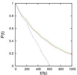
Figure 1: Mean vibrational energy relaxation probability $\langle P(t)\rangle_{S}$ as obtained for NMA in D₂O. Compared is the outcome of direct averaging [Eqs. (15) and (14), red line], cumulant approximation [Eq. (16), green line] and the naive ansatz $\langle P(t)\rangle_{S}=1-\left\langle\rho^{(2)}_{00}(t)\right\rangle_{S}$ (blue line).

II.2 New formulation: Time-dependent driving

In the perturbation theory described above, the vibrational frequencies and coupling elements are assumed to be constant during the VER process.FZS06 ; FS07 This is an assumption which may break down if the time scale of the VER is similar to that of the vibrational parameters. In this work, we extend this formulation by explicitly considering the time dependence of instantaneous vibrational frequencies $\omega_{S}=\omega_{S}(t)$ and $\omega_{\alpha}=\omega_{\alpha}(t)$ and coupling elements $C_{S\alpha\beta}=C_{S\alpha\beta}(t)$ in the derivation of the population probability. As a consequence, the Hamiltonian of system and bath become time-dependent, $H_{S}=H_{S}(t)$ and $H_{B}=H_{B}(t)$, thus yielding the corresponding propagators

$$U_{S}(t) = e^{-(i/\hbar)\int_{0}^{t}H_{S}(\tau)d\tau}\,,$$ (17)

$$U_{B}(t) = e^{-(i/\hbar)\int_{0}^{t}H_{B}(\tau)d\tau}\,.$$ (18)

Second-order time-dependent perturbation theory then leads to an expression that is formally quite similar to Eq. (11), except that the time dependence of all vibrational parameters is considered. The resulting bath correlation function reads

$$\langle\delta F(t_{2})\delta F(t_{1})\rangle_{B} = \frac{\hbar^{2}}{2}\sum_{\alpha,{\beta}}\frac{C_{S\alpha\beta}(t_{2})C_{S\alpha\beta}(t_{1})}{\sqrt{\omega_{\alpha}(t_{2})\omega_{\beta}(t_{1})\omega_{\alpha}(t_{2})\omega_{\beta}(t_{1})}}$$ (19)

$$\times\exp\left\{-i\int_{t_{1}}^{t_{2}}[\omega_{\alpha}(\tau)+\omega_{\beta}(\tau)]d\tau\right\},$$

and we obtain for the time-dependent ground-state population probability

$$\rho^{(2)}_{00}(t) = \frac{\hbar}{2}\sum_{\alpha,\beta}\int^{t}_{0}dt_{2}\int^{t_{2}}_{0}dt_{1}\frac{C_{S\alpha\beta}(t_{2})C_{S\alpha\beta}(t_{1})}{\sqrt{\omega_{S}(t_{2})\omega_{S}(t_{1})\omega_{\alpha}(t_{2})\omega_{\beta}(t_{1})\omega_{\alpha}(t_{2})\omega_{\beta}(t_{1})}}$$ (20)

$$\times\cos\int_{t_{1}}^{t_{2}}[\omega_{S}(\tau)-\omega_{\alpha}(\tau)-\omega_{\beta}(\tau)]d\tau\;.$$

The mean VER probability in Eq. (15) is again defined by averaging over all conformation-dependent probabilities obtained from various MD trajectories. Equation (20) represents the main theoretical result of this paper. We refer to this result as “dynamic treatment” of VER, because it takes into account the time-dependent fluctuations of the environment. Assuming constant frequencies and couplings, we of course recover Eq. (13), which can be regarded as the inhomogeneous limit of Eq. (20).

II.3 Calculation of time-dependent frequencies

In the formulation of VER developed above, we need to calculate instantaneous vibrational frequencies $\omega_{i}(t)$ and couplings $C_{S\alpha\beta}(t)$ along an MD trajectory. As the VER of the amide I mode also involves the vibrations of the first water shell of the peptide, we include NMA and the 16 nearest water molecules in the normal mode analysis (see Sec. II.4 below; the effect of the size of the included solvent shell is discussed in Fig. 6). There are several ways to calculate the normal modes of this subsystem for an instantaneous molecular conformation. As adopted in Refs. FZS06, ; FS07, , for example, one may simply perform an instantaneous normal mode calculation at this molecular geometry. Alternatively, one may first perform a partial geometry optimization of NMA (i.e., keeping the 16 solvent water fixed), before the normal mode calculation is done.

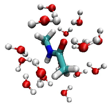
Figure 2: MD snapshot of N-methylacetamide (NMA) and its 16 nearest water molecules.

The latter procedure is sometimes referred to as “quenched normal modes” method,OT90 and is based on the underlying adiabatic approximation for the calculation of the (high-frequency) amide I mode. To explain this, we consider the standard Born-Oppenheimer approach to molecular electronic structures. Here the nuclear (i.e., slow) degrees of freedom coordinates are fixed, while the Schrödinger equation for the electronic (i.e., fast) degrees of freedom is solved. In a direct analogy, to calculate the structure of high-frequency vibrational modes, we keep the slow solvent degrees of freedom fixed and solve the problem of the fast degrees of freedom. Within the harmonic approximation, the latter amounts to a geometry optimization of the subsystem followed by a normal mode calculation.

II.4 Simulation details

All simulations were performed using the CHARMM simulation program package.CHARMM We employed the CHARMM22 all-atom force fieldCHARMMFF to model the solute NMA (H₃C-COND-CH₃) and the TIP3P water modelTIP3P with doubled hydrogen masses to model the solvent D₂O. We also performed simulations for fully deuterated NMA (D₃C-COND-CD₃). The peptide was placed in a periodic cubic box of (25.5 Å)³ containing 551 D₂O molecules. All bonds containing hydrogen bonds were constrained by SHAKE algorithm SHAKE with a relative geometric tolerance of 10^-9. We used a 10 Å  cutoff with a switching function for the nonbonded interaction calculations. After a standard equilibration protocol, we ran a 100 ps NVT trajectory at 300 K, from which 100 statistically independent configurations were sampled. For each initial condition, a 1 ps NVE run was performed for the VER calculations, using a time step of 1 fs.

For the normal mode calculations, the Hessian matrix with respect to the mass-weighted Cartesian coordinates $x_{i}$

$$K_{ij}=\frac{1}{\sqrt{m_{i}m_{j}}}\frac{\partial^{2}V}{\partial x_{i}\partial x_{j}}$$ (21)

of the system NMA/(D₂O)₁₆ was calculated by using the vib command of CHARMM. We obtain in total 180 normal modes. In the partial minimization scheme, the cons fix sele command was employed to constrain all atoms of water except NMA. The min command was used to minimize the energy of the subsystem NMA. The cubic couplings $C_{S\alpha\beta}$ with respect to the normal modes $q_{i}$ were calculated from the Hessian matrix using numerical differentiationFBS05

$$C_{S\alpha\beta} = -\frac{1}{2}\frac{\partial^{3}V}{\partial q_{S}\partial q_{\alpha}\partial q_{\beta}}$$ (22)

$$\simeq -\frac{1}{2}\sum_{ij}U_{i\alpha}U_{j\beta}\frac{K_{ij}(\Delta q_{S})-K_{ij}(-\Delta q_{S})}{2\Delta q_{S}},$$

where $\{U_{i\alpha}\}$ comprises the eigenvectors of the Hessian matrix. To avoid problems with low-frequency bath modes whose frequency may become zero (or even imaginary in the case of instantaneous normal modes) in the denominator of Eqs. (13) and (20), we only include bath modes with $\omega_{\alpha}\geq$ 100 cm^-1.

III Computational results

III.1 Time-dependent frequencies

Let us first consider the time-dependent vibrational frequencies along a typical trajectory by performing instantaneous normal mode analysis of NMA and its 16 nearest water molecules. Figure 3 (top panels) shows the time evolution of the amide I mode (mode 141) and several other modes that are of importance in the VER of the amide I mode (see Table 2 below). The vibrational frequencies obtained from the normal mode calculations at the instantaneous (not minimized) molecular structures (left panel) are seen to undergo substantial fluctuations. The range of fluctuations appears quite unrealistic, when compared to typical experimental infrared line widths. The right panel of Fig. 3 shows results obtained from normal mode calculations for partially minimized molecular structures. We see that the partial geometry optimization of the subsystem NMA/(D₂O)₁₆ results in a reduction of the frequency fluctuations to a physically reasonable range. This finding indicates – in accordance with the underlying adiabatic approximation – that normal mode calculations should be performed after partial geometry optimization rather than at the instantaneous molecular structure. The same conclusion was reached in a recent study of the VER of isolated NMA on ab initio potential energy surfaces.FYHSS08

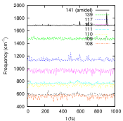
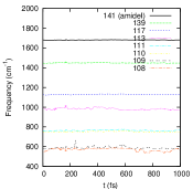
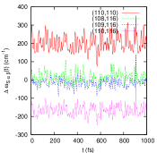
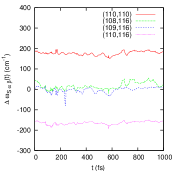
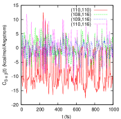
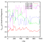
Figure 3: Time evolution of the vibrational dynamics of NMA in D₂O, as obtained from instantaneous normal mode analysis with (right) and without (left) partial energy minimization. Shown are (upper panels) the normal mode frequencies $\omega_{i}$ of selected vibrational modes, (middle panels) the frequency mismatch $\Delta\omega_{S\alpha\beta}(t)=\omega_{S}(t)-\omega_{\alpha}(t)-\omega_{\beta}(t)$ for several resonant bath mode combinations, and (lower panels) the corresponding third-order anharmonic couplings $C_{S\alpha\beta}(t)$.

To assess the effect of the frequency fluctuations on the VER of the amide I mode, we next consider the time dependence of the resonance condition $\Delta\omega_{S\alpha\beta}(t)=\omega_{S}(t)-\omega_{\alpha}(t)-\omega_{\beta}(t)$. As is evident from Eqs. (13) and (20), the minima of $|\Delta\omega_{S\alpha\beta}(t)|$ largely determine the efficiency of the VER process. Adopting the most important mode combinations $\{S,\alpha,\beta\}$ in the VER of the amide I mode of NMA (see Table 1 below), Fig. 3 (middle panels) compares the time evolution of $\Delta\omega_{S\alpha\beta}(t)$ obtained from normal mode calculations with (right) and without (left) partial geometry optimization of the subsystem NMA. The considerable differences found for the two results of $\Delta\omega_{S\alpha\beta}(t)$ again underlines the importance of using the appropriate (i.e., partially minimized) normal mode frequencies.

Also shown in Fig. 3 are the cubic couplings $C_{S\alpha\beta}(t)$ associated with the VER process. From their definition in Eq. (22), it is clear that this quantity, too, depends on how the normal modes are calculated. As expected, we find that the results for $C_{S\alpha\beta}(t)$ without minimization fluctuate much more compared to the results after the partial minimization. We note that apart from the frequencies we also need the normal mode eigenvectors to calculate $C_{S\alpha\beta}(t)$. For simplicity, however, we have assumed that the character of the modes does not change significantly during the VER process and therefore neglected the explicit time dependence of the eigenvectors. This assumption may break down, when it is applied to strongly fluctuating instantaneous normal modes.

III.2 Numerical evaluation of the dynamic VER formula

We are now in a position to study the outcome of the various theoretical treatments of VER introduced above. To this end, Fig. 4 shows the VER probability $P(t)$ of the amide I mode for ten representative trajectories (thin line) as well as the mean population averaged over 60 trajectories (thick line). We again compare results obtained from normal mode calculations with (right) and without (left) partial geometry optimization of the subsystem NMA. Furthermore, the dynamic treatment [Eq. (20)] as well as its inhomogeneous limit [Eq. (13)] are considered. In all cases, we find three stages of the time evolution of $P(t)$. First, we observe a quadratic initial decay for $t\lesssim$ 10 fs, which can be directly derived as short-time expansion of Eq. (13). This is followed by an approximately linear decay for times up to $\approx$ 200 fs. Corresponding to a frequency uncertainty of $\Delta\omega\approx$ 50 cm^-1, this is the time scale on which the normal mode spectrum $\{\omega_{i}\}$ of the “total” system (NMA/(D₂O)₁₆) appears continuous, because $\Delta\omega\gtrsim\omega_{S}-\omega_{\alpha}-\omega_{\beta}$. At longer times, the discrete nature of the bath becomes apparent, leading to dispersion of the population probability for various MD trajectories.

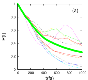
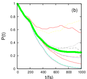
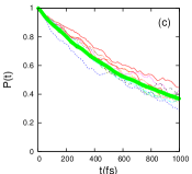
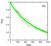
Figure 4: Amide I mode relaxation probability $P(t)$ of NMA, as obtained from an instantaneous normal mode analysis with (right) and without (left) partial energy minimization. Shown are results from (upper panels) the inhomogeneous averaging approximation and (lower panel) dynamics averaging. The VER times according to Eq. (23) are (a) $\tau=0.54\pm 0.23$ ps, (b) $\tau=0.43\pm 0.15$ ps, (c) $\tau=0.93\pm 0.15$ ps, and (d) $\tau=0.60\pm 0.16$ ps.

As may be expected, the different time dependence of the normal mode frequencies with and without the partial minimization also results in different time evolutions of the VER probability. However, the stronger fluctuations of the frequencies and couplings obtained from the calculations without minimization (see Fig. 3) do not necessarily result in enhanced fluctuations of $P(t)$. More important is whether the time-dependent fluctuations are taken into account in the perturbative calculation. After $\gtrsim$ 100 fs, we observe that the inhomogeneously approximated VER probabilities largely disperse, while the dynamic treatment leads to comparatively similar population decays for various MD trajectories. This is because in the former case we use a constant resonance condition $\omega_{S}=\omega_{\alpha}+\omega_{\beta}$, which may differ significantly for individual trajectories. In the dynamic treatment, on the other hand, the time integration in Eq. (20) smoothens the time-dependent resonance condition $\omega_{S}(t)=\omega_{\alpha}(t)+\omega_{\beta}(t)$. To roughly quantify the VER dynamics, we introduce an average time scale $\tau$ viaFS07

$$\frac{1}{\tau}=-\frac{1}{t_{2}-t_{1}}\int_{t_{1}}^{t_{2}}\frac{dP(t)}{dt}\,dt=-\frac{P(t_{2})-P(t_{1})}{t_{2}-t_{1}},$$ (23)

with $t_{1}=0.0$ ps and $t_{2}$=0.5 ps. (Quite similar results are obtained for $t_{1}=0.5$ ps and $t_{2}$=1.0 ps.) As noted in the caption of Fig. 4, we find that the relaxation time $\tau$ as well as its fluctuation may depend significantly on the theoretical treatment of VER.

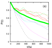
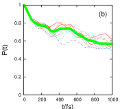
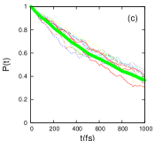
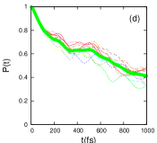
Figure 5: Same as in Fig. 4, but for fully deuterated NMA. The VER times are (a) $\tau=0.89\pm 0.69$ ps, (b) $\tau=1.64\pm 0.32$ ps, (c) $\tau=0.96\pm 0.28$ ps, and (d) $\tau=1.09\pm 0.32$ ps.

It is instructive to compare the above results with calculations for fully deuterated N-methylacetamide. As shown in Fig. 5, deuteration significantly affects the relaxation. While there are again clear differences between the various theoretical treatments, the trends are not that clear as in the case of singly deuterated NMA shown in Fig. 4. Since deuteration may change normal mode frequencies as well as vibrational couplings, this rises the question on the relaxation pathway underlying the VER of NMA.

Table 1: Dominant energy flow pathways of singly deuterated NMA (upper panel) and fully deuterated NMA (lower panel). The vibrational energy relaxation from of the initially excited amide I mode ($\omega_{S}$) to the vibrational modes $\omega_{\alpha}$ and $\omega_{\beta}$ is characterized by their path-specific relaxation times $\tau_{S\alpha\beta}$ (in ps), time-averaged Fermi resonance parameter $\langle F_{S\alpha\beta}\rangle$, frequency mismatch $\langle\Delta\omega_{S\alpha\beta}\rangle$ (in cm^-1), and 3rd order coupling element $\langle C_{S\alpha\beta}\rangle$ (in kcal/mol/Å), respectively.

Mode $\alpha,\beta$	109,116	108,116	109,115	109,117	110,116	112,112	108,117	108,114	109,114
$\tau_{S\alpha\beta}$	3.3	3.6	6.5	7.1	17.5	18.7	21.0	43.2	44.7
$\langle F_{S\alpha\beta}\rangle$	0.209	0.176	0.109	0.043	0.033	0.046	0.055	0.030	0.028
$\langle\Delta\omega_{S\alpha\beta}\rangle$	9.5	17.9	14.6	37.8	164.6	46.0	21.5	56.0	37.0
$\langle C_{S\alpha\beta}\rangle$	2.7	4.2	2.1	2.3	8.4	3.1	1.6	2.2	1.4

Mode $\alpha,\beta$	116,116	109,116	110,116	108,116	109,119	081,109	076,116	079,116	075,109
$\tau_{S\alpha\beta}$	24.6	26.3	33.5	57.7	78.7	80.9	107.2	108.9	142.8
$\langle F_{S\alpha\beta}\rangle$	0.046	0.054	0.096	0.017	0.008	0.002	0.003	0.002	0.002
$\langle\Delta\omega_{S\alpha\beta}\rangle$	252.3	151.2	60.1	172.7	94.6	937.0	565.4	546.9	974.7
$\langle C_{S\alpha\beta}\rangle$	18.9	10.1	7.7	3.6	0.93	0.91	1.2	1.0	0.9

Following definition (23) of an average relaxation time scale $\tau$, the individual energy flow pathways can be characterized by introducing a path-specific VER decay times $\tau_{S\alpha\beta}$. (Note that $1/{\tau}=\sum_{\alpha\beta}1/{\tau_{S\alpha\beta}}$.) Adopting again the sample trajectory shown in Fig. 3, Table 1 lists the dominant relaxation pathways characterized by the shortest $\tau_{S\alpha\beta}$. In the case of singly deuterated NMA, two mode combinations [($\alpha,\beta)$ = (108,116) and (109,116)] results in particularly fast relaxation. To further analyze the relaxation mechanism, we consider the time-averaged Fermi resonance parameter defined asFYHS07 ; FYHSS08

$$\langle F_{S\alpha\beta}\rangle = \left\langle\sqrt{\frac{\hbar}{8{\omega}_{S}\omega_{\alpha}\omega_{\beta}}}\right\rangle\frac{\langle|C_{S\alpha\beta}|\rangle}{\langle|\Delta\omega_{S\alpha\beta}|\rangle},$$ (24)

where $\langle\ldots\rangle$ denotes the time average over a single trajectory. We see that in most (but not all) cases a large Fermi resonance parameter $\langle F_{S\alpha\beta}\rangle$ also means a short corresponding relaxation time $\tau_{S\alpha\beta}$. Furthermore, it is interesting to note that it is the resonance factor $\Delta\omega_{S\alpha\beta}$ rather than the anharmonic coefficient $C_{S\alpha\beta}$ that mostly determines $F_{S\alpha\beta}$ and thus the relaxation pathway.FYHS07 ; FYHSS08

In the case of fully deuterated NMA, on the other hand, there are no such strongly resonant modes. Instead we find that the subpicosecond decay of the overall VER probability $P(t)$ is the result of numerous decay channels with relatively long path-specific decay times. The weak oscillations seen in Fig. 5 reflect the detuning $\Delta\omega_{S\alpha\beta}\approx$ 200 cm^-1 of the two most important paths. Although quite similar in simulation and experiment,HLH98 ; ZAH01 ; Tokmakoff06 interestingly, the mechanism of amide I VER is different for singly and fully deuterated NMA.

Table 2: Characterization of the normal modes that mainly participate in the vibrational energy relaxation of singly deuterated NMA (upper panel) and fully deuterated NMA (lower panel). Shown are the vibrational frequency $\omega_{\alpha}$ and various projections on atomic coordinates, see Eq. (25). Mode 141 is the amide I mode.

Mode #	107	108	109	110	111	112	113	116	117	139	140	141
$\langle\omega_{\alpha}\rangle$ (cm-1)	454	571	590	752	765	864	983	1093	1129	1448	1570	1681
$P_{\rm CO}$	0.16	0.25	0.27	0.39	0.37	0.00	0.12	0.15	0.19	0.36	0.09	0.92
$P_{\rm ND}$	0.10	0.51	0.33	0.28	0.39	0.63	0.04	0.11	0.39	0.16	0.15	0.04
$P_{\rm CH_{3}(C)}$	0.28	0.18	0.31	0.27	0.16	0.00	0.83	0.32	0.18	0.22	0.01	0.04
$P_{\rm CH_{3}(N)}$	0.16	0.05	0.07	0.05	0.08	0.36	0.02	0.42	0.24	0.26	0.75	0.00
$P_{\rm Water}$	0.31	0.02	0.02	0.00	0.00	0.00	0.00	0.00	0.00	0.00	0.00	0.00

Mode #	107	108	109	110	111	112	113	116	117	139	140	141
$\langle\omega_{\alpha}\rangle$ (cm-1)	433	549	560	651	686	787	798	963	1010	1293	1485	1675
$P_{\rm CO}$	0.08	0.28	0.29	0.10	0.17	0.03	0.19	0.49	0.07	0.00	0.46	0.94
$P_{\rm ND}$	0.04	0.21	0.40	0.34	0.20	0.36	0.23	0.13	0.12	0.00	0.39	0.04
$P_{\rm CH_{3}(C)}$	0.12	0.40	0.25	0.41	0.23	0.37	0.42	0.30	0.43	0.00	0.05	0.02
$P_{\rm CH_{3}(N)}$	0.08	0.10	0.03	0.14	0.40	0.23	0.16	0.07	0.38	0.00	0.11	0.00
$P_{\rm Water}$	0.69	0.02	0.03	0.01	0.00	0.00	0.00	0.00	0.00	1.00	0.00	0.00

To characterize the normal modes that mainly participate in the VER process, we have calculated their projection on various atoms of NMA and the surrounding water molecules. For example, the projection of normal mode $\alpha$ onto the CO bond is defined by

$$P_{\rm CO}=\sum_{i\in{\rm CO\,bond}}U_{i\alpha}^{2},$$ (25)

where the sum goes over the $x,y,$ and $z$ coordinates of the corresponding C and O atoms, respectively, and $\{U_{i\alpha}\}$ comprises the eigenvectors of the Hessian matrix [see Eq. (22)]. Listing these projections, Table 2 shows that the resonant modes are mainly localized on NMA, rather than on the solvent water. We also notice that deuteration red-shifts some of the lower frequencies, as expected, but not the amide I mode frequency. This appears to be the main reason of the little resonance of the fully deuterated case.

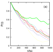
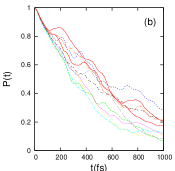
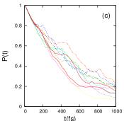
Figure 6: Influence of the solvent on the amide I mode relaxation in NMA. Including 16 (left), 32 (middle), or all (right) water molecules in the calculations, the resulting overall vibrational energy relaxation appears to be quite similar. In the case of isolated NMA (thick line in left panel), however, the relaxation probability $P(t)$ follows the solution-phase decay only up to $\approx$ 300 fs. Note that in the absence of solvent molecules, all trajectories coincide.

To further study the influence of the solvent, Fig. 6 compares the VER dynamics of NMA, when various numbers of D₂O molecules are included in the normal mode and subsequent VER calculations. In all cases, we show the VER probability of 10 single trajectories for singly deuterated NMA, obtained from the dynamic VER treatment and partial energy minimization. Including 16 and 32 water molecules, the resulting amide I relaxation appears to be quite similar [Fig. 6 (a) and (b)]. As another test, we furthermore took into account the remaining 535 water molecules as fixed charges [Fig. 6 (c).] Although individual relaxation pathways may be different, the figure indicates that the first solvation shell with 16 water molecules is sufficient to account for the first step of VER of the amide I mode. Also shown in the left panel of Fig. 6 is the case of isolated NMA. In the absence of solvent water, we find that the excited state population probability $P(t)$ follows the solution-phase decay only up to $\approx$ 300 fs, and deviates to a larger value at longer times. This is a consequence of the fact that while at short times a few resonant pathways dominate, there are numerous possibilities of “off-resonant pathways” that may contribute at longer times.

Finally we remark on the comparison of the above results with existing experimental data. For both singly and fully deuterated NMA, biphasic relaxation $P_{\rm exp}(t)=pe^{-t/\tau_{1}}+(1-p)e^{-t/\tau_{2}}$ of the amide I mode has been reported.HLH98 ; ZAH01 ; Tokmakoff06 The relaxation times are $\tau_{1}$ = 0.45 ps ($p=0.8$) and $\tau_{2}$ = 4 ps for the singly deuterated NMA,ZAH01 and $\tau_{1}$ = 0.38 ps ($p=0.5$) and $\tau_{2}$ = 2.1 ps for the fully deuterated NMA.Tokmakoff06 Comparing $P_{\rm exp}(t)$ with our results obtained from the dynamic VER treatment and partial energy minimization, Fig. 7 shows excellent agreement between theory and experiment – maybe better as it can be expected from a simple force field modeling of the normal modes of the system. Independent of force field uncertainties, however, is our finding that the VER of the amide I mode in NMA consists of two phases (see also Figs. 4 and 5). This is because for $t\lesssim$ 200 fs the system’s spectral density appears continuous due to the frequency-time uncertainty relation, while at longer times the discrete nature of the bath becomes apparent. Although it is tempting to speculate that this behavior can explain the experimentally obtained biphasic relaxation of NMA, it is at present not clear if the approximations involved in our description allow for this conclusion. (E.g., the validity of time-dependent perturbation theory deteriorates at longer times.) Nevertheless, the observation that amide I relaxation in larger peptides occurs in a monoexponential mannerHLH98 is consistent with the fact that the above described effect is expected to vanish for larger peptides with higher spectral density.

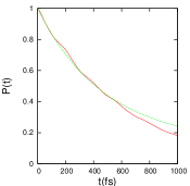
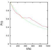
Figure 7: Comparison of calculated (red lines) and experimental (green lines) results for the VER of the amide I mode in NMA. Shown are data for singly (left) and fully (right) deuterated NMA.

IV Concluding Remarks

We have outlined a computational approach to describe the energy relaxation of a high-frequency vibrational mode in a fluctuating heterogeneous environment. Extending the previous work,FZS06 we have employed second time-dependent perturbation theory, which includes the fluctuations of the parameters in the Hamiltonian within the vibrationally adiabatic approximation. This means that the time-dependent vibrational frequencies along an MD trajectory are obtained via a partial geometry optimization of the peptide with fixed solvent water and a subsequent normal mode calculation. Although it requires more computational effort, the partial geometry optimization is necessary, because its omission results in unrealistically high fluctuations of the vibrational frequencies and other quantities (see Fig. 3).

Adopting the amide I VER of NMA in heavy water as a test problem, we have shown that the inclusion of dynamic fluctuations may significantly change the time evolution of the VER probability $P(t)$ (see Fig. 4). After $\gtrsim$ 200 fs, we observe that the inhomogeneously approximated VER probabilities largely disperse, while the dynamic treatment leads to comparatively similar population decays for various MD trajectories. This is because in the former case we use a constant resonance condition $\omega_{S}=\omega_{\alpha}+\omega_{\beta}$, while the time integration in the dynamic treatment averages over the time-dependent resonance condition.

To characterize the dominant energy flow pathways of the amide I VER of NMA, we have introduced path-specific VER decay times and considered the Fermi resonance parameter of the relaxation process. In the case of singly deuterated NMA, mainly two combinations of bath modes were found to achieve the vibrational relaxation. In the case of fully deuterated NMA, on the other hand, we have not observed such strongly resonant modes. Instead we found that the subpicosecond decay of the overall VER probability $P(t)$ is the result of numerous decay channels with relatively long path-specific decay times. In both cases, we observed that the VER of the amide I mode in NMA consists of two phases (see Fig. 4). This is because for $t\lesssim$ 200 fs the system’s spectral density appears continuous due to the frequency-time uncertainty relation, while at longer times the discrete nature of the bath becomes apparent. Considering our excellent agreement between theory and experiment (see Fig. 7), it may be speculated if this behavior can explain the experimentally obtained biphasic relaxation of NMA.

Two directions for further researches are apparent. On a short time scale (here $\lesssim$ 200 fs), our results suggest that a single normal mode calculation should be sufficient to describe VER in peptides. The restriction to ultrashort time scales therefore allows us to employ high-quality ab initio methods to calculate the vibrational structure of even large molecules.FYHS07 ; FYHSS08 On a longer time scale (here $\gtrsim$ 500 fs), on the other hand, the validity of time-dependent perturbation theory is expected to deteriorate. As a straightforward extension, the vibrational dynamics may be described by stochastic Schrödinger equations GNKS07 or stochastic Liouville equations.Hanggi ; Tanimura06

- (1) P.K. Agarwal, S.R. Billeter, P.R. Rajagopalan, S.J. Benkovic, and S. Hammes-Schiffer, Proc. Natl. Acad. Sci. USA 301, 2794 (2002); P. Agarwal, J. Am. Chem. Soc. 127, 15248 (2005); A. Jiménez, P. Clapés, and R. Crehuet, J. Mol. Model (2008), doi:10.1007/s00894-008-0283-2.
- (2) J.I. Steinfeld, J.S. Francisco, and W.L. Hase, Chemical Kinetics and Dynamics, Prentice-Hall (1989).
- (3) D.M. Leitner and P.G. Wolynes, Chem. Phys. Lett. 280, 411 (1997).
- (4) M. Gruebele and P.G. Wolynes, Acc. Chem. Res. 37, 261 (2004); M. Gruebele, J. Phys.: Condens. Matter 16, R1057 (2004).
- (5) R.J.D. Miller, Ann. Rev. Phys. Chem. 42, 581 (1991); R.J. Dwayne Miller, Can. J. Chem. 80, 1 (2002); A.M. Nagy, V.I. Prokhorenko, R.J.D. Miller, Curr. Opin. Struct. Biol. 16, 654 (2006).
- (6) Y. Mizutani and T. Kitagawa, Science 278, 443(1997); Y. Mizutani and T. Kitagawa, Chem. Record 1, 258 (2001).
- (7) P. Hamm, M.H. Lim, R.M. Hochstrasser, J. Phys. Chem. B 102, 6123 (1998).
- (8) M.T. Zanni, M.C. Asplund, R.M. Hochstrasser, J. Chem. Phys. 114, 4579 (2001).
- (9) L.P. DeFlores, Z. Ganim, S.F. Ackley, H.S. Chung, A. Tokmakoff, J. Phys. Chem. B 110, 18973 (2006).
- (10) M.D. Fayer, Ann. Rev. Phys. Chem. 52, 315 (2001).
- (11) J.C. Deàk, S.T. Rhea, L.K. Iwaki, and D.D. Dlott, J. Phys. Chem. A 104, 4866(2000).
- (12) S. Nishida, T. Nada and M. Terazima, Biophys. J. 89, 2004 (2005).
- (13) S. Woutersen and P. Hamm, J. Phys.: Condens. Matter 14, R1035 (2002); P. Hamm, J. Helbing, and J. Bredenbeck, Annu. Rev. Phys. Chem. 59, 291 (2008).
- (14) D.W. Oxtoby, Adv. Chem. Phys. 40, 1 (1979); Adv. Chem. Phys. 47, 487 (1981); Ann. Rev. Phys. Chem. 32, 77 (1981).
- (15) V.M. Kenkre, A. Tokmakoff, and M.D. Fayer, J. Chem. Phys. 101, 10618 (1994).
- (16) R. Rey, K.B. Moller, and J.T. Hynes, Chem. Rev. 104, 1915 (2004); K.B. Moller, R. Rey, and J.T. Hynes, J. Phys. Chem. A 108, 1275 (2004).
- (17) C.P. Lawrence and J.L. Skinner, J. Chem. Phys. 117, 5827 (2002); ibid. 117, 8847 (2002); ibid. 118, 264 (2003); A. Piryatinski, C.P. Lawrence, and J.L. Skinner, ibid. 118, 9664 (2003); ibid. 118, 9672 (2003); C.P. Lawrence and J.L. Skinner, ibid. 119, 1623 (2003); ibid. 119, 3840 (2003).
- (18) E.L. Sibert and R. Rey, J. Chem. Phys. 116, 237 (2002); T.S. Gulmen and E.L. Sibert, J. Phys. Chem. A 109, 5777 (2005); S.G. Ramesh and E.L. Sibert, J. Chem. Phys. 125 244512 (2006); S.G. Ramesh and E.L. Sibert, ibid. 125 244513 (2006).
- (19) R. Ramirez, T. Lopez-Ciudad, P. Kumar, and D. Marx, J. Chem. Phys. 121, 3973 (2004).
- (20) D.E. Sagnella and J.E. Straub, Biophys. J. 77, 70 (1999); L. Bu and J.E. Straub, ibid. 85, 1429 (2003).
- (21) R.M. Whitnell, K.R. Wilson, and J.T. Hynes J. Chem. Phys. 96, 5354 (1992).
- (22) E.R. Henry, W.A. Eaton, R.M. Hochstrasser, Proc. Natl. Acad. Sci. USA 83, 8982 (1986).
- (23) D. E. Sagnella and J. E. Straub, J. Phys. Chem. B 105, 7057 (2001); L. Bu and J. E. Straub, ibid. 107, 10634 (2003); L. Bu and J. E. Straub, ibid. 107, 12339 (2003); Y. Zhang, H. Fujisaki, and J. E. Straub, ibid. 111, 3243 (2007).
- (24) P.H. Nguyen and G. Stock, J. Chem. Phys. 119, 11350 (2003); P. H. Nguyen and G. Stock, Chem. Phys. 323, 36 (2006); P. H. Nguyen, R. D. Gorbunov, and G. Stock, Biophys. J. 91, 1224 (2006); A. Moretto, M. Crisma, C. Toniolo, P. H. Nguyen, G. Stock, and P. Hamm, Proc. Natl. Acad. Sci. USA 104, 12749 (2007).
- (25) K. Moritsugu, O. Miyashita and A. Kidera, Phys. Rev. Lett. 85, 3970, (2000); J. Phys. Chem. B, 107, 3309 (2003).
- (26) I. Okazaki, Y. Hara, and M. Nagaoka, Chem. Phys. Lett. 337, 151 (2001); M. Takayanagi, H. Okumura, and M.Nagaoka, J. Phys. Chem. B, 111, 864 (2007).
- (27) S. Okazaki, Adv. Chem. Phys. 118, 191 (2001); M. Shiga and S. Okazaki, J. Chem. Phys. 109, 3542 (1998); ibid. 111, 5390 (1999); T. Mikami, M. Shiga and S. Okazaki, ibid. 115, 9797 (2001); T. Terashima, M. Shiga, and S. Okazaki, ibid. 114, 5663 (2001); Mikami, T.; Okazaki, S. ibid. 119, 4790 (2003); T. Mikami and S. Okazaki, ibid. 121, 10052 (2004); M. Sato and S. Okazaki, ibid. 123, 124508 (2005); M. Sato and S. Okazaki ibid. 123, 124509 (2005).
- (28) Q. Shi and E. Geva, J. Chem. Phys. 118, 7562 (2003); Q. Shi and E. Geva, J. Phys. Chem. A 107, 9059 (2003); Q. Shi and E. Geva, ibid. 107, 9070 (2003); B.J. Ka, Q. Shi, and E. Geva, ibid. 109, 5527 (2005); B.J. Ka and E. Geva, ibid. 110, 13131 (2006); I. Navrotskaya and E. Geva, ibid. 111, 460 (2007); I. Navrotskaya and E. Geva, J. Chem. Phys. 127, 054504 (2007).
- (29) H. Fujisaki, L. Bu, and J.E. Straub, Adv. Chem. Phys. 130B, 179 (2005); H. Fujisaki and J.E. Straub, Proc. Natl. Acad. Sci. USA 102, 6726 (2005).
- (30) D.M. Leitner, Adv. Chem. Phys. 130B, 205 (2005); D.M. Leitner, Phys. Rev. Lett. 87, 188102 (2001); X. Yu and D.M. Leitner, J. Chem. Phys. 119, 12673 (2003); X. Yu and D.M. Leitner, J. Phys. Chem. B 107, 1689 (2003); D.M. Leitner, M. Havenith, and M. Gruebele, Int. Rev. Phys. Chem. 25, 553 (2006).
- (31) A.G. Dijkstra, T. la Cour Jansen, R. Bloem, and J. Knoester, J. Chem. Phys. 127, 194505 (2007).
- (32) H. Fujisaki, Y. Zhang, and J.E. Straub, J. Chem. Phys. 124, 144910 (2006).
- (33) H. Fujisaki and J.E. Straub, J. Phys. Chem. B 111, 12017 (2007).
- (34) H. Fujisaki, K. Yagi, K. Hirao, and J.E. Straub, Chem. Phys. Lett. 443, 6 (2007).
- (35) H. Fujisaki, K. Yagi, K. Hirao, J.E. Straub, and G. Stock, submitted.
- (36) U. Weiss, Quantum Dissipative Systems, 2nd ed. World Scientific (1999); C.W. Gardiner and P. Zoller, Quantum Noise, 3rd ed. Springer (2004); D.F. Walls and G.J. Milburn, Quantum Optics, 2nd ed. Springer (2008).
- (37) H.-P. Breuer and F. Petruccione, The Theory of Open Quantum Systems, Oxford University, New York (2002).
- (38) A. Nitzan, Chemical Dynamics in Condesed Phase: Relaxation, Transfer, and Reactions in Condensed Molecular Systems, Oxford (2006).
- (39) H. J. Bakker, J. Chem. Phys. 121, 10088 (2004).
- (40) I. Goychuk and P. Hänggi, Adv. Phys. 54, 525 (2005).
- (41) A. Ishizaki and Y. Tanimura J. Chem. Phys. 125, 084501 (2006); A. Ishizaki and Y. Tanimura ibid. 123, 014503 (2005).
- (42) T. Yu, L. Diosi, N. Gisin, and W.T. Strunz, Phys. Lett. A 265, 331 (2000); G. Schaller and T. Brandes, e-print arXiv:0804.2374.
- (43) I. Ohmine and H. Tanaka, J. Chem. Phys. 93, 8138 (1990); I. Ohmine and H. Tanaka, Chem. Rev. 93, 2545 (1993).
- (44) B.R. Brooks, R.E. Bruccoleri, B.D. Olafson, D.J. States, S. Swaminathan, and M. Karplus, J. Comp. Chem. 4, 187 (1983); A.D. MacKerell, Jr., B. Brooks, C.L. Brooks, III, L. Nilsson, B. Roux, Y. Won, and M. Karplus, The Encyclopedia of Computational Chemistry 1. Editors, P.v.R. Schleyer et al. Chichester: John Wiley & Sons. 271 (1998).
- (45) A.D. MacKerell Jr., D. Bashford, M. Bellott, R.L. Dunbrack, J.D. Evanseck, M.J. Field, S. Fischer, J. Gao, H. Guo, S. Ha, D. Joseph-McCarthy, L. Kuchnir, K. Kuczera, F.T.K. Lau, C. Mattos, S. Michnick, T. Ngo, D.T. Nguyen, B. Prodhom, W.E. Reiher, B. Roux, M. Schlenkrich, J.C. Smith, R. Stote, J.E. Straub, M. Watanabe, J. Wiorkiewicz-Kuczera, D. Yin, and M. Karplus, J. Phys. Chem. B 102, 3586 (1998).
- (46) W.L. Jorgensen, J. Chandrasekhar, J. Madura, R.W. Impey, and M.L. Klein, J. Chem. Phys. 79, 926 (1983).
- (47) J.-P. Ryckaert, G. Ciccotti, and H.J.C. Berendsen, J. Comp. Phys. 23, 327 (1977).
- (48) R.D. Gorbunov, P.H. Nguyen, M. Kobus, and G. Stock, J. Chem. Phys. 126, 054509 (2007); M. Kobus, R. D. Gorbunov, P. H. Nguyen, and G. Stock, Chem. Phys. 347, 208 (2008).
- (49) Y. Tanimura, J. Phys. Soc. Jpn. 75, 082001 (2006).