Shaping Robust System through Evolution
Kunihiko Kaneko11footnotemark: 122footnotemark: 2
Department of Basic Science, Univ. of
Tokyo, 3-8-1 Komaba, Tokyo 153-8902, Japan
22footnotemark: 2 ERATO Complex Systems Biology Project, JST, 3-8-1
Komaba, Tokyo 153-8902, Japan
Abstract
Biological functions are generated as a result of developmental dynamics that form phenotypes governed by genotypes. The dynamical system for development is shaped through genetic evolution following natural selection based on the fitness of the phenotype. Here we study how this dynamical system is robust to noise during development and to genetic change by mutation. We adopt a simplified transcription regulation network model to govern gene expression, which gives a fitness function. Through simulations of the network that undergoes mutation and selection, we show that a certain level of noise in gene expression is required for the network to acquire both types of robustness. The results reveal how the noise that cells encounter during development shapes any network’s robustness, not only to noise but also to mutations. We also establish a relationship between developmental and mutational robustness through phenotypic variances caused by genetic variation and epigenetic noise. A universal relationship between the two variances is derived, akin to the fluctuation-dissipation relationship known in physics.
Lead paragraph
Biological function is generally robust to noise in dynamical systems and to mutation to structure of the system. How are these two types of robustness related? Through numerical simulations of a minimal model that captures the essence of a gene expression dynamics that undergoes a mutation and selection process, we demonstrate that the evolved networks acquire robustness to mutation only when gene expression is sufficiently noisy - a physical constraint highlighted by a series of experimental studies in recent years. We derive a quantitative condition for evolution of robustness which ultimately links robustness to mutation in the evolutionary time-scale and robustness to noise in development in the reproductive time-scale. Our model simulations predict correlation between the two robustness, which lead to a universal proportionality relationship between variances of genetic and epigenetic phenotype fluctuations, which remind us of fluctuation-dissipation relationship in statistical physics.
1 Introduction
Function in a biological system is generated by dynamical systems in general. A specific shape of a protein that gives rise to some function is formed by folding dynamics. In a cell, gene expression pattern changes in time, to shape some chemical composition, from which a given function of the cell emerges. In multicellular organisms, developmental dynamics lead to patterns of differentiated cells. Phenotype is shaped in a broad sense from such ‘developmental dynamical systems’, according to which the fitness of an individual is determined.
In a biological system, such developmental dynamics are shaped through Darwinian evolution. Offspring are produced depending on the fitness of the parents, with some variations that introduce slight modifications in parameters or networks in developmental dynamical systems. Among modified dynamical systems, phenotypes with higher function are selected for the next generation. Hence, evolutionary shaping of function is a result of variation and selection of developmental dynamical systems.
Combining both the terminology of biology and dynamical systems, evolutionary process is summarized as follows. (i) The genotype gives a set of equations, i.e., terms and parameters in developmental dynamical systems. (ii) From an initial condition, the developmental dynamical system leads to a set of state variables for a phenotype. (iii) Fitness is a function of these state variables. The offspring number increases with fitness. (iv) In reproduction, there are mutations (or other sources for variations) giving rise to variation in dynamical systems. At each generation, there is redistribution of dynamical systems. If evolution serves to increase fitness, dynamical systems with higher function are shaped through this selection-mutation process.
In discussing this evolutionary shaping of dynamical systems with higher function, an important issue is robustness. Robustness is defined as the ability to function against changes in the parameters of a given system [1, 2, 3, 4, 5, 6]. In any biological system, these changes have two distinct origins: genetic and epigenetic. The former concerns structural robustness of the phenotype, i.e., rigidity of phenotype against variation in dynamical systems, introduced by genetic changes produced by mutations. On the other hand, the latter concerns robustness against the stochasticity that can arise in a given dynamical system, which includes fluctuation in initial states and stochasticity occurring during developmental dynamics or in the external environment. For example, stochasticity in gene expression has recently been studied extensively both experimentally and theoretically [7, 8, 9, 10, 11]. Indeed, the existence of such stochasticity is natural, because the number of molecules in a cell is generally limited. Accordingly, phenotypes of cells differ, even among those sharing the same genotype[12]. An important recent recognition is that phenotypic noise is indeed significant, as is highlighted by the log-normal distribution of protein abundances in bacteria[9].
The two types of robustness—epigenetic and genetic—are concerned with fluctuations in phenotype caused by noise in developmental processes and by variations in dynamical systems caused by genetic changes. In terms of dynamical systems, these two types of robustness are the stability of a state (an attractor) to external noise and the structural stability of the state against changes in the underlying equations, respectively. Then, how are these two forms of robustness related in evolution? Recently we have found a possible relationship between the two, from an experiment on adaptive evolution in bacteria[13] and numerical evolution of reaction networks and transcription regulation networks[5, 14]. The two types of robustness, measured by the (inverse of) phenotypic variances, increase in correlation through evolution, whereas evolutionary speed is greater as the magnitude of the phenotypic fluctuation due to noise is increased. Hence, the relevance of noise to evolution is suggested.
Despite recent quantitative observations on phenotypic fluctuation, noise is often thought to be an obstacle in tuning a system to achieve and maintain a state with higher functions, because the phenotype may be deviated from an optimal state achieving a higher function through such noise. Indeed, the question most often asked is how a given biological function can be maintained in spite of the existence of phenotypic noise[11, 15]. Although the positive roles of stochasticity in gene expression to cell differentiation [16] and adaptation have been discussed [17, 18], its role in evolution has not been explored fully. As a relatively large amount of phenotypic noise has been preserved through evolution, it is important to investigate any positive roles of such noise for the evolution of biological functions.
The present paper is organized as follows. Following the Ref.[5], we introduce a simple transcription regulation network model in §2. In this model. fitness is determined by the gene expression pattern generated by this network. Using a genetic algorithm to change the network so that the fitness is increased, we show that evolution of the robustness of fitness to mutation to a given network is possible only under a certain level of noise in the gene expression dynamics. Dependence of the fitness distribution on the noise level is analyzed in §3. Variances of fitness due to developmental noise and to genetic variation are computed, which give indices for developmental and mutational robustness, respectively. The proportional relationship between the two variances is given in §4, whereas in §5, the two variances are computed for the expression of all genes, which demonstrate common proportion relationship, suggesting the existence of a universal relationship akin to fluctuation-dissipation theorem in statistical physics. Summary and discussion are given in §6.
2 Model
To study evolutionary shaping of dynamical systems, we consider a simple model for ‘development’. This consists of a complex dynamic process to reach a target phenotype under a condition of noise that might alter the final phenotypic state. We do not choose a biologically realistic model that describes a specific developmental process, but instead take a model as simple as possible to satisfy the minimal requirement for our study. Here we take a simplified model for gene expression dynamics, governed by transcription regulatory networks. Expression of a gene activates or inhibits expression of other genes under noise. These interactions between genes are determined by the transcription regulatory network (TRN). The expression profile changes in time, and eventually reaches a stationary pattern. This gene expression pattern determines fitness.
To be specific, a typical switch-like dynamics with a sigmoid input–output behavior [19, 20, 21] was adopted, although several simulations in the form of biological networks will give essentially the same result. In this simplified model, the dynamics of a given gene expression level is described by:
| (1) |
where , and is Gaussian white noise given by . is the total number of genes, and is the number of output genes that are responsible for fitness to be determined. The value of represents noise strength that determines stochasticity in gene expression. By following a sigmoid function , has a tendency to approach either 1 or -1, which is regarded as ‘on’ or ‘off’ in terms of gene expression. The initial condition is given by (-1,-1,…,-1); i.e., all genes are off unless noted otherwise.
Depending on the expression pattern, the cell state changes. Hence, the function of the cell and accordingly its fitness changes. Here we assume that fitness is determined by setting a target gene expression pattern. In the present paper we adopt a simple target so that the gene expression levels () for the output genes reach ‘on’ states, i.e., . The fitness is at its maximum if all genes are ‘on’ after a transient time span , and at its minimum if all are off. is set at , if all the target genes are on, and is decreased by 1 if one of the genes is ‘off’. Accordingly, the fitness function is defined by
| (2) |
where for and otherwise. The initial time can be considered as the time required for developmental dynamics. The fitness is computed only after time , which is sufficiently large for a given gene expression’s dynamics to fall on an attractor. In the simulations presented here we adopt and the results to be discussed are not altered even if it is increased. Here, in considering also the possibility of an oscillatory attractor, we adopt the temporal average for the fitness, but indeed, it is not necessary as attractors after evolution are mostly fixed points. is set at here, but even if it is defined just by a snapshot value at , the results are not essentially altered.
Selection is applied after the introduction of mutation at each generation in the TRN. Among the mutated networks, we select those with higher fitness values. Because the network is governed by which determines the ‘rule’ of the dynamics, it is natural to treat as a measure of genotype. Individuals with different genotype have a different set of .
As model (1) contains a noise term, the fitness can fluctuate at each run, which leads to a distribution in , even among individuals sharing the same network. For each individual network, we compute the average fitness over a given number of runs. At each generation there are individuals with different sets of . Then we select the top networks that have higher fitness values.
At each generation there are individuals. We compute the average fitness for each network by carrying out runs for each. Then, networks with higher values of are selected for the next generation, from which is ‘mutated’, i.e., for a certain pair selected randomly with a certain fraction is changed among . (To be specific, only the changes are allowed). The fraction of path change is given by the mutation rate . Unless otherwise mentioned, only a single path, i.e., a single pair of is changed so that the mutation rate . Here we make mutants from each of the top networks, to keep networks again for the next generation. Following mutation, the individuals at each generation have slightly different network elements, , so that the values of differ. From this population of networks we repeat the processes of developmental dynamics, their mutation, and selection of networks with higher fitness values.
Unless otherwise mentioned, we chose , while the conclusion to be shown does not change as long as these are sufficiently large. (We have also carried out the selection process by instead of , but the conclusion is not altered if is chosen to be sufficiently large.) Throughout the paper, we use . For most numerical results we use and , unless otherwise mentioned. Initially we chose randomly with equal probability for . However, the results to be discussed are not changed qualitatively, even if the fraction of 0 is increased. As shown in eq.(1), we did not include a connection from the output genes , so that with is fixed at 0 and is not mutated. However, the results to be discussed are not altered, even if such connections are included in eq.(1).
3 Decrease in the average fitness with the decrease of noise
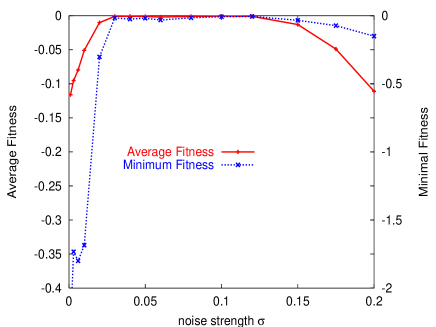
Let us first see how the evolutionary process changes as a function of the noise strength . Within a hundred generations, the top fitness among the network population approaches the highest value , if noise level is not too high ( for ) (see Fig. 1). However, this is not the case for the average fitness among a population with slightly different genes. For low noise level, average fitness stays lower than the fittest value. In the middle range of noise level, the average value approaches the fittest value. This difference against the noise level is clearer in the temporal evolution of the lowest fitness among the existing networks. As shown in Fig. 1, the value stays rather low for a small noise case, whereas for evolution under a high noise value, it goes up with the top fitness value. In other words, the distribution of the fitness over existing networks has three distinct behaviors, depending on the noise strength .
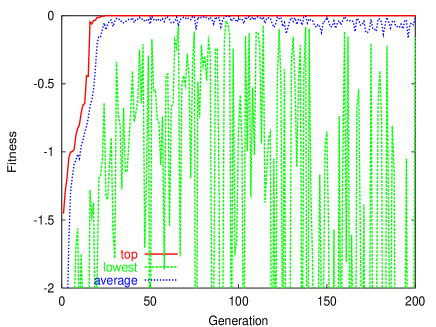
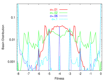
(i) For small ( for and the mutation rate with 1 path per generation), the distribution is broad. The top reaches the fittest, although there remain individuals with very low fitness values , even after many generations of evolution.
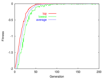
(ii) For the middle range (), the distribution is sharp and concentrated at the fittest value. Even those individuals with the lowest fitness approach . We call this range the ‘robust evolution region’.
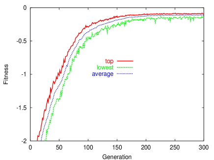
(iii) For the much larger noise value (), the top does not reach the fittest values, while the distribution is sharp, and concentrated around the top value. Here the noise is so large that changes its sign at a certain fraction even after reached the target, so that the top fittest is not achieved.
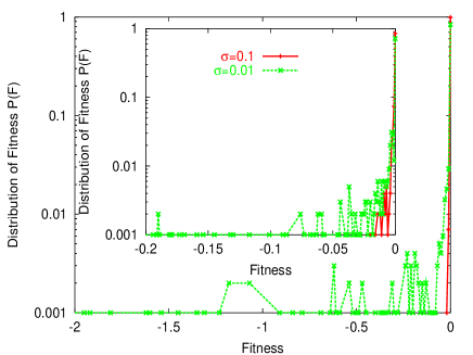
The change in the distribution between (i) and (ii) is demonstrated in Fig. 2. There is a threshold noise , below which the distribution is broadened. As a result, the average fitness over all individuals, is low. and the lowest fitness values over individuals , after a sufficiently large number of generations, are plotted against in Figure 3. The abrupt decrease in fitness suggests the existence of threshold noise level , below which low-fitness mutants always remain in the distribution.
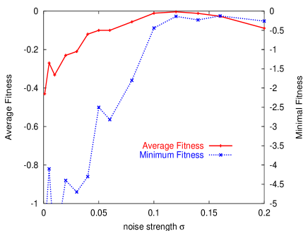
This transition on the noise level is rather sharp, as long as the number of genes is large. As becomes smaller, the plateau in the highest fitness value against is decreased, and the transition loses sharpness, as shown in Fig. 4 for , with the mutation rate per single path change per generation. With an increase in , the region achieving the highest fitness with sharp distribution increases, as well as the increase in the sharpness of transition.
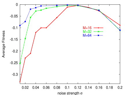
If there are more genes, change in a single path has a smaller influence, so that an increase in the robust evolution region is to be expected. However, the increase in the robust region with is not solely caused by the decrease in the effective mutation rate. In Fig. 5, we have changed the number of genes , by fixing the mutation rate per path, i.e., a single path change per generation for , 4 paths for , and 16 for . Even in this fixed mutation rate, the transition is sharper, and the increase in the robustness in the evolution is detected.
Of course, the increase in the mutation rate reduces the robust evolution region. Comparing Fig. 2(a) and Fig. 4 shows that the threshold noise level for the robust evolution region is lowered with the decrease in mutation rate, where the mutation rate is 16 times higher for the simulation for in Fig. 4 than that for Fig. 2(a).
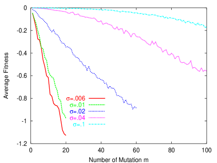
At the transition at we discuss here, mutational robustness of the evolved network changes. The top fitness network evolved at a low noise level () does not have robustness against mutation, in contrast to those evolved at a higher noise level. To check this distinction statistically, we measured the average fitness of mutants generated from the top fitness. We took a network with the top fitness evolved after generations, and changed paths randomly (i.e., change in a value of among ,0). By making a thousand networks of such mutations, we have measured the average fitness of such mutants, which is plotted against in Fig. 6. For , the average fitness decreases linearly with the number of added mutations , as . The coefficient decreases with the increase in , and for , the linear decrease component vanishes, giving rise to a plateau around . In other words, the fitness landscape has an almost neutral region. The fitness is rather insensitive to mutation, demonstrating the evolution of mutational robustness. Around , estimated at small mutation number is rather small, and we may expect that as , although careful examination of the slope at limit is needed to confirm it.
The transition with regards to the mutational robustness at reminds us of the error catastrophe introduced by Eigen and Schuster[22], since the population of non-fit mutants starts to accumulate after this transition. In their error catastrophe, the transition occurs when the advantage by fitted individuals cannot overcome combinatorial diversity of non-fit mutants. Their error catastrophe occurs with the increase in the mutation rate, while our robustness transition occurs with the decrease in developmental noise. In our case, the transition is of dynamic origin, as will be discussed in the next section, whereas there exist (combinatorially) much more non-fit networks than the fittest ones. The robustness transition here could be related with (or regarded as an extension of) error catastrophe, but the relationship between the two remains to be clarified.
4 Dynamic origin of the robustness transition
Why does the system not maintain the highest fitness state under a condition of small phenotypic noise ? Indeed, the top fitness networks that evolved under low noise have dynamic behaviors distinct from those that evolved under high noise. First, the highest fitness network evolved at low often fails to reach the target if simulated under a higher noise level. The expression level often exhibits a few oscillations before reaching the target state and noise might cause expression of the output genes to switch to ‘off’ states. In contrast, the temporal course of gene expression evolved for is much smoother, and is not affected by noise. This distinction is confirmed by simulating gene expression dynamics by cutting off the noise term over a variety of initial gene expression conditions, and to check if the orbit is attracted to the original target. We found that, for networks evolved under , a large portion of the initial conditions is attracted into the target pattern, while for those evolved under , only a tiny fraction (i.e., the vicinity of all ‘off’ states) is attracted to the target (see Fig. 6).
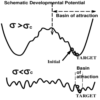
If the time course of a given gene expression to reach its final pattern is represented as a motion falling along a potential valley, our results suggest that the potential landscape becomes smoother and simpler through evolution and loses ruggedness after a few hundred generations. This ‘developmental’ landscape is displayed schematically in Fig. 7. For networks evolved under there is a large, smooth attraction to the target, whereas for the dynamics evolved under , the initial states are split into small basins, from each of which the gene expression patterns reach different steady states.
Now, consider the mutation to a network. Any change in the network leads to slight alterations in gene expression dynamics. In smooth dynamics, as in Fig. 7(a), this perturbation influences the attraction to the target only slightly. By contrast, under the dynamics as shown in Fig. 7(b), a slight change easily destroys the attraction to the target attractor. For this latter case, the fitness of mutant networks is distributed down to lower values, which explains the behavior observed in Fig. 3.
Accordingly, evolution to eliminate ruggedness in developmental potential is possible only for sufficient noise amplitude, whereas ruggedness remains for small noise values and the developmental dynamics often fail to reach the target, either by noise in gene expression dynamics or by mutations to the networks. It is interesting to note that a greater set of initial conditions is attracted to a target pattern for networks evolved under conditions of high noise. Existence of such global attraction in an actual gene network has recently been reported for the yeast cell cycle[23].
5 Evolution of robustness
According to our results in the two previous sections, a network evolved under high noise has two types of robustness. The target pattern is reached even if the developmental dynamics are perturbed by noise or by a mutation to the network. The fitness is rather insensitive to both of such perturbations.
As an index for robustness, variance of the fitness (or phenotype) is useful[5]. There are two types of variance corresponding to the above two types of robustness, i.e., genetic and epigenetic robustness. Variance corresponding to genetic change, denoted by , is defined as phenotype variance caused by the distribution of genes;
| (3) |
where we note is the distribution of average fitness over all networks at each generation, and is the average of average fitness over all networks.
As the variance decreases, the system increases its robustness to genetic change (mutation). On the other hand, epigenetic robustness is measured by the phenotypic variance of isogenic organisms . Indeed, the phenotypes of isogenic individual organisms fluctuate, as discussed extensively[7, 8, 9, 10, 11]. We define the isogenic phenotypic variance by
| (4) |
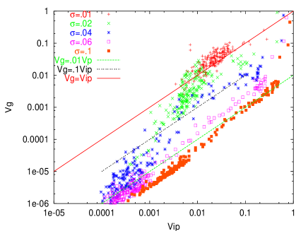
where is the fitness distribution among isogenic individuals sharing the same network , and is the average fitness of the genotype . generally depends on the individual (genotype) . As a measure of , we adopted such that gives the peak in the fitness distribution , i.e., most typical genotype. Or, instead, we estimated it by the average of over all genotypes existing at each generation. The overall - relationship is not altered between the two estimates. In Fig.8, we adopted the latter estimate, to reduce statistical error.
Under high noise conditions, the selection process favors a developmental process that is robust against it. This robustness to noise is then embedded into robustness against mutation. Indeed, for , both and decrease through the course of evolution (Fig. 8), while maintaining proportionality between the two. Such proportionality between the two has been discussed from an evolutionary stability analysis under a few assumptions[14, 24, 25]. For , the the inequality is satisfied, while it is broken at the transition , which also agrees with the theoretical analysis. On the other hand, the proportionality between and is also consistent with an observation on an experiment in bacterial evolution [13], if the Fisher’s theorem[26, 27, 28] on the proportionality between evolution speed and is applied.
6 Consolidation of the Expression of Non-target Genes

So far we have studied how a dynamical system consisting of positive and negative feedbacks is shaped to generate a given target output pattern. Here, the matrix has a large number of nonzero elements, and generally the structure is complex. Fitness generated from such a complex network is robust to noise and to mutation. How is such a robust system achieved to fixate the expressions of target genes?
In our model, there are more degrees of freedom (genes) besides those for the target genes. The expression levels of the non-target genes do not influence the fitness, and can take either positive or negative values. Hence, there is no selection pressure leading them to be fixed, or robust to noise or to mutation. However, we have found that expression levels of many (about half) non-target genes are fixed to positive or negative values successively through the course of evolution in the robust evolution region, i.e., for . Even after mutation to values, the sign value of does not change for most genes (data not shown). For such genes, the variance of each expression level over mutants becomes rather small because of evolution.
To check for a possible decrease in the variance of expression levels, we define for gene , as the variance of computed at , (i.e., after the time span for development) over individuals with different genes, instead of the variance of fitness we measured in the last section. ( is the average among isogenic individuals, i.e., the average over runs). In other words, is defined by replacing by in eq.(3). This variance is plotted in Fig. 9 as a function of generation. Here, for , the variance of the expression level of the target genes decreases at an earlier generation, together with a few other genes, followed by a decrease in for about half of the others towards low levels. Indeed, after 200 generations of evolution, the variance for about half of the genes is less than . Expression levels of many degrees of freedom other than the requested degrees of freedom as a target are also fixed. This consolidation is relevant to achieve a robust system. Indeed, for , such fixation of non-target gene expression levels is not observed.
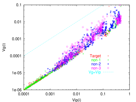
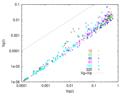
Similarly to , we define as the isogenic variance for each , by using instead of in eq. (4), and have computed its evolution over generations. For genes which show the decrease in , the variances also decrease through evolution. Furthermore, for such genes , and decrease in proportion, as shown in Fig. 10(a). The proportionality relationship between and holds true not only for fitness but also for many genes, including non-target ones. Surprisingly, as evolution progresses, the plot of approaches a single line, suggesting that the proportion coefficient between the two approaches the same value for all genes, whose gene expressions are fixated to on or off by generation. In fact, we have plotted for all genes in Fig. 10(b). For each given generation, the overlaid plot of fits on the same line for most genes. In other words, the proportion relationship between the two variances holds not only for each gene’s expression through the course of evolution, but also for expression levels over different genes at each generation. Over generations, the plots shift toward smaller values , approaching a unique line. This ‘universal’ coefficient for all genes suggests the existence of a global potential dynamic system governing many gene expression patterns.
7 Summary and Discussion
We have shown here that a dynamical system that is robust both to noise and to structural variation is shaped through evolution under noise. In our study, robustness to developmental noise and to mutation are represented quantitatively in terms of the phenotypic variance of isogenic organisms and by genetic variation . The proportionality between the two through evolution is a quantitative manifestation of how developmental and mutational robustness can evolve in coordination. In fact, whether these two types of robustness emerge under natural selection has long been debated in the context of developmental dynamics and evolution theory[1, 2, 29, 30], since the propositions of stabilization selection by Schmalhausen[31] and canalization by Waddington[32, 33] more than half a century ago. Here we have demonstrated a correlation between developmental robustness to noise and genetic robustness to mutation, and have shown that the former leads to the latter.
Isogenic phenotypic fluctuation is related to phenotypic plasticity, which is a degree of phenotype change in a different environment. Positive roles for phenotypic plasticity in evolution have been discussed elsewhere [30, 34, 35, 36]. Because susceptibility to environmental changes and phenotypic fluctuation are correlated positively according to the fluctuation–response relationship[24], our present results on the relationship between phenotypic fluctuations and evolution imply a relationship between phenotypic plasticity and evolution akin to the genetic assimilation proposed by Waddington[32].
Although we have demonstrated this evolution of robustness using a network model of transcriptional regulation, we expect this behavior to be observable generally if fitness is determined through developmental dynamics that are sufficiently complex so that a given developmental process, when deviated by noise, may fail to reach the fittest target pattern. In fact, the decrease in phenotypic variance as well as the proportionality law between and has been confirmed in a catalytic reaction network model[14].
We have also found that the expression of many non-target genes is also fixed. The behavior of many other degrees of freedom is consolidated with that directly related to fitness. With this consolidation, the system’s behavior is constrained to exhibit an identical phenotype against noise and mutation. Many degrees of freedom are highly correlated, which possibly results in the emergence of a simple set of global dynamics over many gene expressions. The existence of a universal proportionality between and with an identical proportion coefficient over many genes might be a manifestation of such global dynamics. It is interesting to note that this universal proportionality over components is also observed in a reaction network model for a reproducing cell[37].
During the course of evolution, the variance levels of some gene expressions decrease at an early generation, while others decrease only later. This difference between genes should be related to how their expressions influence those for the target. It will be important to study the order of fixation in terms of the network structure.
Borrowing the concept from statistical physics, we previously proposed an evolutionary fluctuation–response relationship, where proportionality between evolution speed (response) and isogenic fluctuations is proposed and experimentally verified. As the speed of evolution is proportional to according to Fisher’s fundamental theorem of natural selection[26, 27],the relationship then suggested the proportionality between and . Note that in physics, the proportion coefficient between response and fluctuation is represented universally in terms of temperature, and is known as the fluctuation–dissipation relation[38, 39] or Einstein’s relation[40]. Discovery of our universal proportion coefficient over genes suggests the existence of a general theory akin to the fluctuation–dissipation theorem that could be applied to evolutionary biology and also to robust design of dynamical systems.
In the present paper, we adopted a simple fitness condition favoring a fixed expression of target genes. Accordingly, such system that has a large basin for a fixed point attractor corresponding to the target pattern is evolved. It should be of importance to examine a case with a more complex fitness condition. A straightforward extension is the use of several target patterns depending on some inputs applied to some genes. Another extension is the use of fitness favoring for dynamic attractors. As the model (1), with suitable choice of , shows periodic or chaotic attractors[41], study on the evolution of robust dynamic system is also of importance ( see also [42]).
I would like to thank Chikara Furusawa, Koichi Fujimoto, Masashi Tachikawa, Shuji Ishihara, Tetsuya Yomo, and Satoshi Sawai for stimulating discussion.
References
- [1] de Visser J.A., et al.: ‘Evolution and detection of genetic robustness’, Evolution, 2003, 57, pp. 1959–1972.
- [2] Wagner A.: ‘Robustness against mutations in genetic networks of yeast’, Nature Genetics, 2000, 24, pp. 355–361.
- [3] Barkai N., and Leibler S.: ‘Robustness in simple biochemical networks’, Nature, 1997, 387, pp. 913–917.
- [4] Alon U., Surette M.G., Barkai N., and Leibler S.: ‘Robustness in bacterial chemotaxis’, Nature, 1999, 397, pp. 168–171.
- [5] Kaneko K.: ‘Evolution of robustness to noise and mutation in gene expression dynamics’, PLoS ONE, 2007, 2, p. e434.
- [6] Ciliberti S., Martin O.C., and Wagner A.: ‘Robustness can evolve gradually in complex regulatory gene networks with varying topology’, PLOS Comp. Biology, 2007, 3, p. e15.
- [7] Elowitz, M.B., Levine, A.J., Siggia, E.D., and Swain, P.S.: ‘Stochastic gene expression in a single cell’, Science, 2002, 297 pp. 1183–1187.
- [8] Hasty, J., Pradines, J., Dolnik, M., and Collins, J.J.: ‘Noise-based switches and amplifiers for gene expression’, Proc. Natl. Acad. Sci. U S A, 2000, 97, pp. 2075–2080.
- [9] Furusawa, C., Suzuki, T., Kashiwagi, A., Yomo, T., and Kaneko, K.: ‘Ubiquity of log-normal distributions in intra-cellular reaction dynamics’, Biophysics, 2005, 1, pp. 25–31.
- [10] Bar-Even A., et al.: ‘Noise in protein expression scales with natural protein abundance’, Nature Genetics, 2006, 38, pp. 636–643.
- [11] Kaern, M., Elston, T.C., Blake, W.J., and Collins, J.J.: ‘Stochasticity in gene expression: from theories to phenotypes’, Nat. Rev. Genet., 2005, 6, pp. 451–464.
- [12] Spudich J.L., and Koshland, D.E., Jr.: ‘Non-genetic individuality: chance in the single cell’, Nature, 1976, 262, pp. 467–471.
- [13] Sato, K., Ito, Y., Yomo, T., and Kaneko, K.: ‘On the relation between fluctuation and response in biological systems’, Proc. Nat. Acad. Sci. U S A, 2003, 100, pp. 14086–14090.
- [14] Kaneko, K. and Furusawa, C.: ‘An evolutionary relationship between genetic variation and phenotypic fluctuation’, J. Theo. Biol., 2006, 240, pp. 78–86.
- [15] Ueda, M., Sako, Y., Tanaka, T., Devreotes, P., and Yanagida, T.: ‘Single-molecule analysis of chemotactic signaling in Dictyostelium cells’, Science, 2001, 294, pp. 864–867.
- [16] Kaneko, K. and Yomo, T.: ‘Isologous diversification for robust development of cell society’, J. Theor. Biol., 1999, 199, pp. 243–256.
- [17] Kashiwagi, A., Urabe, I., Kaneko., K., and Yomo, T.: ‘Adaptive response of a gene network to environmental changes by attractor selection’, PLoS ONE, 2006, 1, p. e49.
- [18] Furusawa, C. and Kaneko, K.: ‘A generic mechanism for adaptive growth regulation’, PLoS Computational Biology, 4(2008) e3.
- [19] Glass, L., and Kauffman, S.A.: ‘The logical analysis of continuous, non-linear biochemical control networks’, J. Theor. Biol., 1973, 39, pp. 103–129.
- [20] Mjolsness, E., Sharp, D.H., and Reisnitz, J.: ‘A connectionist model of development’, J. Theor. Biol., 1991, 152, pp. 429–453.
- [21] Salazar-Ciudad, I., Garcia-Fernandez, J., and Sole, R.V.: ‘Gene networks capable of pattern formation: from induction to reaction–diffusion’, J. Theor. Biol., 2000, 205, pp. 587–603.
- [22] Eigen M. and Schuster P. (1979) The Hypercycle, Springer.
- [23] Li, F., Long, T., Lu, Y., Ouyang, Q., and Tang, C.: ‘The yeast cell-cycle network is robustly designed’, Proc. Nat. Acad. Sci. U S A, 2004, 101, pp. 10040–10046.
- [24] Kaneko, K.: ‘Life: An Introduction to Complex Systems Biology’, Springer, Heidelberg and New York, 2006.
- [25] Kaneko, K. and Furusawa, C.: ‘Consistency Principle of a Biological System’, Theoretical Bioscience, in press.
- [26] Fisher, R. A. (1930,1958) The Genetical Theory of Natural Selection, Oxford Univ. Press.
- [27] Edwards, A.W.F., (2000) Foundations of mathematical genetics, Cambridge University Press.
- [28] Futuyma D.J. (1986) Evolutionary Biology (Second edition), Sinauer Associates Inc., Sunderland.
- [29] Ancel, L.W., and Fontana, W.: ‘Plasticity, evolvability, and modularity in RNA’, J. Exp. Zool., 2002, 288, pp. 242–283.
- [30] Kirschner, M.W., and Gerhart J.C.: ‘The Plausibility of Life’, Yale Univ. Press, 2005.
- [31] Schmalhausen, I.I.: ‘Factors of Evolution: The Theory of Stabilizing Selection’, Univ. of Chicago Press, Chicago, 1949 (reprinted 1986).
- [32] Waddington, C.H.: ‘The Strategy of the Genes’, Allen & Unwin, London, 1957.
- [33] Siegal, M.L., and Bergman, A.: ‘Waddington’s canalization revisited: developmental stability and evolution’ Proc Nat. Acad. Sci. U S A, 2002, 99, pp. 10528–10532.
- [34] West-Eberhard M.J.: Developmental Plasticity and Evolution, Oxford Univ. Press, 2003.
- [35] Ancel L.W.: ‘Undermining the Baldwin expediting effect: does phenotypic plasticity accelerate evolution?’, Theor. Popul. Biol., 2000, 58, pp. 307–319.
- [36] Callahan, H.S., Pigliucci, M., and Schlichting, C.D.: ‘Developmental phenotypic plasticity: where ecology and evolution meet molecular biology’, Bioessays, 1997, 19, pp. 519–525.
- [37] Furusawa, C. and Kaneko K.: in preparation.
- [38] Kubo R., Toda M., Hashitsume N. 1985, Statistical Physics II: (English translation; Springer).
- [39] U.M.B. Marconi, A. Puglisi, L. Rondoni, and A. Vulpiani, “Fluctuation-Dissipation: Response Theory in Statistical Physics”, in press.
- [40] Einstein A., Investigation on the Theory of of Brownian Movement, (Collection of papers ed. by R. Furth), Dover, 1956 (republication from 1926).
- [41] see e.g., Lewis L., Glass L. “Steady states, limit cycles, and chaos in models of complex biological networks”, International Journal of Bifurcation and Chaos 1, 477-483 (1991) ; Mason J.P. et al. “Evolving complex dynamics in electronic models of genetic networks”, Chaos 14 (3), 707-715 (2004).
- [42] Sevim V. and Rikvold P.A., Chaotic Gene Regulatory Networks Can Be Robust Against Mutations and Noise, arXiv: q-bio.0711.1522v2, J. theor Biol., in press.