Thermoacoustic tomography with detectors on an open curve: an efficient reconstruction algorithm

Abstract

Practical applications of thermoacoustic tomography require numerical inversion of the spherical mean Radon transform with the centers of integration spheres occupying an open surface. Solution of this problem is needed (both in 2-D and 3-D) because frequently the region of interest cannot be completely surrounded by the detectors, as it happens, for example, in breast imaging. We present an efficient numerical algorithm for solving this problem in 2-D (similar methods are applicable in the 3-D case). Our method is based on the numerical approximation of plane waves by certain single layer potentials related to the acquisition geometry. After the densities of these potentials have been precomputed, each subsequent image reconstruction has the complexity of the regular filtration backprojection algorithm for the classical Radon transform. The peformance of the method is demonstrated in several numerical examples: one can see that the algorithm produces very accurate reconstructions if the data are accurate and sufficiently well sampled, on the other hand, it is sufficiently stable with respect to noise in the data.

Introduction

The thermoacoustic tomography (TAT) is based on measurements of acoustic waves excited in the patient’s body by an external electromagnetic pulse [15, 36]. The method is gaining popularity among researchers because it combines the high resolution of the ultrasound tomography with the high contrast of the images attainable due to the strong variance in the electromagnetic properties of the body tissues. One of the most promising applications of this technique is breast imaging, where absorption of the electromagnetic energy in tumors is several times higher than that in healthy tissues. Under certain simplifying assumptions (most importantly, that of a constant speed of sound in the tissue) the corresponding reconstruction problem can be reduced to the inversion of the spherical mean Radon transform. In the present paper we propose an efficient numerical algorithm for solving this problem in 2-D in the case when the detectors lie on an open curve only partially surrounding the region of interest.

A significant progress has been achieved recently in mathematics of TAT; an extended discussion and relevant references can be found in reviews [1, 12, 16]. In particular, several versions of explicit inversions formulas [11, 12, 18, 37, 8] and certain series solutions [22, 23, 19] have been obtained for measurement schemes with the detectors lying either on closed surfaces surrounding the region of interest (ROI), or on certain open but unbounded surfaces, such as a plane or infinite cylinder.

However, in most applications the ROI is not the whole human body but rather a part of it — as it happens, for example, in mammography. In such situations only some part of the region boundary can be covered by the detectors. This, in turn, necessitates the development of algorithms that can reconstruct the image from such data.

The simplest approach to image reconstruction from open surfaces is to place detectors on a truncated plane or cylinder and to apply the known inversion formula(s) for the full plane or infinite cylinder. Of course, the reconstruction would not be exact; moreover, it has been shown that for a stable reconstruction of a compactly supported function from its spherical means it is necessary to know the integrals over sufficiently many spheres, so that the so-called ”visibility” condition is satisfied [20, 38, 39, 25, 24]. (It have been shown, in particular, that under this condition the reconstruction problem can be reduced either to the inversion of an elliptic operator or, after a certain filtration, to a solution of the Fredholm integral equation of the second kind [24, 25, 27, 17]. In both cases the problem is only mildly unstable, similarly to the inversion of the standard Radon transform [21]). The ”visibility” condition (for TAT) is satisfied if for each point $x$ in the ROI each straight line passing through $x$ intersects the measuring surface at least once. A sphere surrounding the object satisfies this condition while an infinite plane and an infinite cylinder do not. For a truncated plane or truncated cylinder the set of ”bad” directions is even larger than for their infinite counterparts. If this condition is violated, it is practically impossible to accurately reconstruct sharp interfaces (material boundaries) at those points of the image for which some of the straight lines normal to the interface do not intersect the measuring surface. (In 2-D an exact reconstruction technique was developed in [26] for the case when the centers of the integration circles lie on a segment of a straight line. However, the reconstruction is still, in general, unstable in this case.)

For a given bounded ROI there exist many bounded open acquisition surfaces that do satisfy the visibility condition. Almost all known reconstruction techniques applicable to such surfaces are of approximate nature. For example, by ”approximating” the integration spheres by planes and by applying some version of the classical inverse Radon transform, one can reconstruct an ”approximation” to the image. Due to the symmetry in the classical Radon projections, the normals to the integration planes should fill only a half of a unit sphere, making possible the reconstruction from an open measurement surface. A more sophisticated approach is represented by the so-called ”straightening” methods [33, 34] based on the approximate reconstruction of the classical Radon projections from the measurements that correspond to the spherical mean Radon transform. However, these methods do not yield the exact solution but rather a parametrix of the problem; the image is reconstructed only up to a certain smooth term. In other words, while jumps corresponding to sharp material interfaces are reconstructed accurately, the accuracy of the lower spatial frequencies can not be guaranteed. Unlike the approximations resulting from the discretization of the exact inversion formulas (in the situations when such formulas are known), the parametrix approximations do not converge when the discretization of the data is refined (in the absence of noise). In [28], an exact inversion formula for the spherical surface is used to obtain approximate reconstructions from other measurement surfaces; in order to further improve the approximation, additional corrections are introduced. These methods yield different parametrices than the one proposed in [33, 34]; which one is better remains an open question.

An accurate numerical reconstruction from an open surface acquisition scheme was demonstrated in [4] (see also [31]). In this work a version of an iterative algebraic reconstruction algorithm was successfully employed to recover a numerically generated phantom. Iterative algebraic reconstruction algorithms are, however, notoriously slow; the above-mentioned reconstruction, for example, required the use of a cluster of computers and took 100 iterations to converge. A faster converging algorithm can be obtained by combining iterative refining with a parametrix-type algorithm [30, 28]. These methods are closely related to the general scheme proposed in [5] for the inversion of the generalized Radon transform with integration over general manifolds. It reduces the problem to the Fredholm integral equation of the second kind, which is well suited for numerical solution. Such an approach can be viewed as using a parametrix method as an efficient preconditioner for an iterative solver, which, as it has been shown in numerical experiments, significantly accelerates the convergence of the iterations..

Finally, in [32] an interesting attempt has been made to generate the absent data from the consistency conditions on the spherical mean Radon transform, in order to ”numerically close” the open measurement surface. The resulting algorithm, however, seems to be less accurate than methods we mentioned earlier, and it exhibits instability on higher spatial frequencies.

In the present paper we propose a novel non-iterative algorithm for the numerical inversion of the spherical mean Radon transform from open surfaces in 2-D. Our numerical experiments show that this method yields very accurate reconstructions in the absence of noise, and is almost as stable as the classical filtration/backprojection (FBP) algorithm (widely used for the inversion of the regular Radon transform [14, 21]). The present algorithm requires pre-computation of certain functions that jointly serve as a numerical filter; this needs to be done only once for a given configuration of detectors. After these functions have been computed, each reconstruction has numerical complexity similar to that of the FBP.

1 Formulation of the problem

In the thermoacoustic tomography acoustic detectors measure the pressure of the outgoing wave radiating from the patient’s body. This acoustic wave is generated by the thermoacoustic expansion of the tissues initiated by a very short electromagnetic pulse. The initial pressure $f(x)$ strongly depends on the type of tissue, and is significantly higher for tumors, since they happen to absorb much more electromagnetic energy than healthy tissue. Thus, recovering $f(x)$ would yield important medical information about the location and shape of tumors.

Let us denote by $g(z,t)$ the pressure registered at the moment $t$ by the acoustic detector placed at the point $z$. Under certain assumptions (such as a constant sound speed in the body, ideal infinitely small detector, infinitely short pulse, and so on), one can recover from the measurements the integral of $f(x)$ over a sphere of radius $r=ct$ centered at $z.$ A dimensional analysis shows that in order to reconstruct a function of a 3-D variable, the detectors should cover some measurement surface $\Sigma.$ Assuming for simplicity that the speed of sound equals unity, one arrives at the following formulation of the inverse problem: reconstruct function $f(x)$ supported within some 3-D region of interest $\Omega$ from known values of its integrals $g(z,r)$ over all spheres of radius $r$ with centers $z$ lying on surface $S$ ($S$ and $\Omega$ are disjoint sets).

A 2-D version of this problem also arises in the thermoacoustic tomography. Recently, it has been proposed to use integrating linear detectors instead of point-like transducers [6, 29, 7, 28]. One such detector consists of a long straight segment of optical fiber that serves as a sensor of an optical interferometer; the measurements are proportional to the integral the acoustic pressure over the length of the fiber. According to the experimentalists, such detectors have much better sensitivity and spatial resolution than the conventional transducer. It has been shown [6] that the reconstruction problem in this case reduces to the inversion of a set of the circular mean Radon transforms followed by the inversion of a set of the regular 2-D Radon transforms (where the circular mean Radon transform is a set of normalized integrals over circles with centers lying on a curve) The same practical reasons as in 3-D case lead to the requirement that the centers of the integration circles lie on an open bounded curve satisfying (for a given ROI) the ”visibility” condition.

In the present paper we study mostly the 2-D case; in order to simplify the analysis we will concentrate on a truncated circular geometry as described below. The 2-D region of interest $\Omega$ is a truncated disk $\Omega(R,x_{\mathit{right}})=\{x=(x_{1},x_{2})\left|{}\right.x_{1}^{2}+x_{2}^{2}<R^{2}\mathrm{\ and\ }x_{1}<x_{\mathit{right}}\}$ and the centers of integration circles lie on the circular arch $\gamma(R_{\gamma},z_{\mathit{right}})=\{z=(z_{1},z_{2})\left|{}\right.z_{1}^{2}+z_{2}^{2}=R_{\gamma}^{2}\mathrm{\ and\ }z_{1}<z_{\mathit{right}}\},$ where $R_{\gamma}>R,$ see Figure 1. Our goal is to reconstruct a $C_{0}^{1}$ function $f(x)$ supported in $\Omega$ from the known values of its integrals $g(z,r)$ over circles $\mathbb{S}(r,z)$ of radii $r$ centered at points $z\in\gamma$

$$g(z,r)=\int\limits_{\mathbb{S}(r,z)}f(x)dl(x)=r\int\limits_{\mathbb{S}^{1}}f(z+r\varpi)d\varpi.$$

(The circular mean Radon transform is defined by the normalized integrals (or means), i.e. by values of $g(z,r)/2\pi r.$ We, however, prefer to work with the integrals $g(z,r)$ ). The invertibility of the circular mean Radon transform is well known for such geometry [3]. The stability of the reconstruction problem is, again, determined by the ”visibility” condition (see [20, 38, 39, 25, 24]), which for this geometry is equivalent to the inequality $z_{\mathit{right}}\geq x_{\mathit{right}}.$ Our goal is to develop an efficient computational algorithm for the solution of this problem.

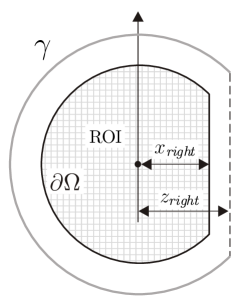
Figure 1: Geometry

2 Outline of the method

The present algorithm is based on precomputing the approximations of plane waves in $\Omega$ by the single layer potentials in the form $\int_{\gamma}Z(\lambda|z-x|)\rho(z)dl(z),$ where $\rho(z)$ is the density of the potential and $Z(t)\$is either the Bessel function $J_{0}(t)$ or the Neumann function $Y_{0}(t).$ Specifically, given a wavevector $\xi$ we find numerically the densities $\rho_{\xi,J}(z)$ and $\rho_{\xi,Y}(z)$ of the potentials

$$W_{J}(x,\rho_{\xi,J}) =\int_{\gamma}J_{0}(\lambda|z-x|)\rho_{\xi,J}(z)dl(z),$$ (1)

$$W_{Y}(x,\rho_{\xi,Y}) =\int_{\gamma}Y_{0}(\lambda|z-x|)\rho_{\xi,Y}(z)dl(z),$$ (2)

where $\lambda=|\xi|,$ such that

$$W_{J}(x,\rho_{\xi,J})+W_{Y}(x,\rho_{\xi,Y})\thickapprox\exp(-i\xi\cdot x),\quad\forall x\in\Omega,$$ (3)

Obtaining such approximations is not trivial; we discuss this issue in more detail in the next section. However, if the densities $\rho_{\xi,J}$ and $\rho_{\xi,Y}$ have been found for all $\xi$ then function $f(x)$ can be easily reconstructed. Indeed, let us introduce convolutions $G_{J}(\lambda,y),$ $G_{Y}(\lambda,z)$ as follows

$$G_{J}(\lambda,z) =\int_{\Omega}f(x)J_{0}(\lambda|z-x|)dx,$$

$$G_{Y}(\lambda,z) =\int_{\Omega}f(x)Y_{0}(\lambda|z-x|)dx.$$

We notice that the boundary values of these functions for all $z\in\gamma$ can be computed from projections $g(z,r)$:

$$G_{J}(\lambda,z) =\int_{R^{+}}g(z,r)J_{0}(\lambda r)dr,$$ (4)

$$G_{Y}(\lambda,z) =\int_{R^{+}}g(z,r)Y_{0}(\lambda r)dr.$$ (5)

Consider now the Fourier transform $\hat{f}(\xi)$ of $f(x)$

$$\hat{f}(\xi)=\frac{1}{2\pi}\int_{\Omega}f(x)\exp(-i\xi\cdot x)dx.$$

Using (3) we obtain

$$\hat{f}(\xi) \thickapprox\frac{1}{2\pi}\int_{\Omega}f(x)\left[W_{J}(x,\rho_{\xi,J})+W_{Y}(x,\rho_{\xi,Y})\right]dx$$

$$=\frac{1}{2\pi}\int_{\gamma}\left[\int_{\Omega}f(x)J_{0}(\lambda|z-x|)dx\right]\rho_{\xi,J}(z)dl(z)$$

$$+\frac{1}{2\pi}\int_{\gamma}\left[\int_{\Omega}f(x)Y_{0}(\lambda|z-x|)dx\right]\rho_{\xi,Y}(z)dl(z)$$

$$=\frac{1}{2\pi}\int_{\gamma}\left[\rho_{\xi,J}(z)G_{J}(\lambda,z)+\rho_{\xi,Y}(z)G_{Y}(\lambda,z)\right]dl(z).$$ (6)

Formulas (4) and (5) in combination with (6) allow us to reconstruct (approximately) the Fourier transform $\hat{f}(\xi)$ of $f(x).$ Now $f(x)$ can be recovered by inverting the 2D Fourier transform. In order to minimize the operation count we will compute $G_{J}(\lambda,z)$ and $G_{Y}(\lambda,z)$ (using (4) and (5)) for a set of fixed values of $\lambda=|\xi|;$ thus, the values of $\hat{f}(\xi)$ will be found on a polar grid in $\xi.$ One can now use a high-order 2-D interpolation to obtain values of the Fourier transform on the Cartesian grid and apply the inverse 2D Fast Fourier Transform (FFT). Another approach is to utilize the famous slice-projection theorem (see, for example [21]) and reconstruct from the values of $\hat{f}(\xi)$ on the polar grid the regular Radon projections of $f(x);$ the function then can be obtained by the application of the FBP algorithm [14, 21]. We have chosen the latter approach. The whole algorithm can be briefly outlined as follows.

1. Choose a uniform polar grid in $\xi.$ For each value of $\xi_{i,j}=\lambda_{i}(\cos\theta_{j},\sin\theta_{j})$ precompute $\rho_{\xi_{i,j},J}$ and $\rho_{\xi_{i,j},Y}$ as described in the next section. This step does not depend on values of $g(z,r)$ and needs to be performed only once for each particular geometry.

2. Given values of $g(z,r),$ compute $G_{J}(\lambda_{i},z)$ and $G_{Y}(\lambda_{i},z)$ (using (4) and (5)) for each value of $i.$ This can be done using the trapezoid rule in $r.$

3. Compute $\hat{f}(\xi_{i,j})$ according to (6), using the same discretization of the integral as was used to obtain (1) and (2).

4. Apply 1-D FFT to values of $\hat{f}(\xi_{i,j})$ for each fixed $j,$ to reconstruct the classical Radon projections of $f(x)$ corresponding to the angular parameter $\theta_{j}.$ (Alternatively, in the presence of strong noise in the data one can introduce a lower-pass filter $\eta(\xi)$ and use $\eta(|\xi_{i,j}|)\hat{f}(\xi_{i,j})$ instead of $\hat{f}(\xi_{i,j})$ on this step).

5. Use the well-know FBP algorithm [14, 21] to reconstruct $f(x)$ from the standard Radon projections.

If we assume, for simplicity, that the size of the reconstruction grid is $n\times n,$ and that the number of detectors and the number of integrals in one projection are of the same order (say, $\mathcal{O}(n)),$ then steps 2, 3, and 5 of the algorithm require $\mathcal{O}(n^{3})$ floating point operations; step 5 is faster ($\mathcal{O}(n^{2}\log n)$ flops). Step 1, described in the next section, is more expensive computationally. The precise operation count depends on the algorithm used to compute $n$ Singular Value Decompositions (SVD) for matrices of size $(n\times n),$ and can be $\mathcal{O}(n^{4})$ operations or higher. However, step 1 needs to be performed only once for each particular geometry. The number of data generated on step 1 and stored on a hard drive (values of the densities $\rho_{\xi_{i,j},J}$ and $\rho_{\xi_{i,j},Y}$) is of order $\mathcal{O}(n^{3}).$ The rest of the algorithm, including reading the precomputed densities, is completed in $\mathcal{O}(n^{3})$ operations (similarly to the FBP).

Obviously, the feasibility of this method hinges on our ability to find approximations in the form (3). In the following section we discuss the existence, accuracy and stability of such approximations.

3 Approximations of plane waves by the single layer potentials

3.1 Full circle acquisition

Before studying the more interesting case of an open acquisition curve $\gamma$ let us consider a simpler case of the full-circle acquisition geometry. Suppose the 2-D region of interest $\Omega$ is the disk of radius $R$ centered at the origin and the detectors lie on the concentric circle $\gamma$ of radius $R_{\gamma}>R$ (this formally corresponds to a particular case when $x_{\mathit{right}}\geq R$ and $z_{\mathit{right}}\geq R_{\gamma}).$ In order to represent the plane wave $\exp(i\xi\cdot x)$ by the single layer potentials supported on $\gamma$, we expand the wave in the Fourier series in polar angle $\theta_{x}$ as follows:

$$\exp(i\xi\cdot x)=\sum_{n=-\infty}^{+\infty}i^{n}J_{|n|}(\lambda|x|)\exp(in\left[\theta_{x}-\theta_{\xi}\right]))$$ (7)

where $\xi=\lambda(\cos\theta_{\xi},\sin\theta_{\xi}),$ $x=|x|(\cos\theta_{x},\sin\theta_{x})$ (this is a well known Jacobi-Anger expansion [9, 35]). We also utilize the addition theorem [9, 35] for the Hankel function $H_{0}^{(1)}(\cdot)=J_{0}(\cdot)+iY_{0}(\cdot)$:

$$H_{0}^{(1)}(\lambda|x-z|)=\sum_{n=-\infty}^{+\infty}H_{|n|}^{(1)}(\lambda|z|)J_{|n|}(\lambda|x|)\exp(in\left[\theta_{x}-\theta_{z}\right]),$$ (8)

where $z=|z|(\cos\theta_{z},\sin\theta_{z}).$ By integrating equation (8) with the density $\exp(in\theta_{z})$ supported on $\gamma$ one obtains

$$\int_{\gamma}H_{0}^{(1)}(\lambda|z-x|)\exp(in\theta_{z})dl(z)=2\pi R_{\gamma}H_{|n|}^{(1)}(\lambda R_{\gamma})J_{|n|}(\lambda|x|)\exp(in\theta_{x})$$

or

$$\overline{H_{|n|}^{(1)}(\lambda R_{\gamma})}\int_{\gamma}H_{0}^{(1)}(\lambda|z-x|)\exp(in\theta_{z})dl(z)=2\pi R_{\gamma}\left|H_{|n|}^{(1)}(\lambda R_{\gamma})\right|^{2}J_{|n|}(\lambda|x|)\exp(in\theta_{x}).$$

The latter expression can be used to express the cylindrical wave $J_{|n|}(\lambda|x|)\exp(in\theta_{x})$ in the form

$$J_{|n|}(\lambda|x|)\exp(in\theta_{x}) =\frac{J_{|n|}(\lambda R_{\gamma})}{2\pi R_{\gamma}\left|H_{|n|}^{(1)}(\lambda R_{\gamma})\right|^{2}}\int_{\gamma}J_{0}(\lambda|z-x|)\exp(in\theta_{z})dl(z)$$

$$+\frac{Y_{|n|}(\lambda R_{\gamma})}{2\pi R_{\gamma}\left|H_{|n|}^{(1)}(\lambda R_{\gamma})\right|^{2}}\int_{\gamma}Y_{0}(\lambda|z-x|)\exp(in\theta_{z})dl(z).$$

Further, by substituting this formula into Jacobi-Anger expansion (7), one can represent $\exp(i\xi\cdot x)$ as the sum of the single layer potentials

$$\exp(i\xi\cdot x) =\frac{1}{2\pi R_{\gamma}}\int_{\gamma}\left[\sum_{n=-\infty}^{+\infty}\frac{J_{|n|}(\lambda R_{\gamma})}{\left|H_{|n|}^{(1)}(\lambda R_{\gamma})\right|^{2}}i^{n}\exp(in\left[\theta_{z}-\theta_{\xi}\right]))\right]J_{0}(\lambda|z-x|)dl(z)$$

$$+\frac{1}{2\pi R_{\gamma}}\int_{\gamma}\left[\sum_{n=-\infty}^{+\infty}\frac{Y_{|n|}(\lambda R_{\gamma})}{\left|H_{|n|}^{(1)}(\lambda R_{\gamma})\right|^{2}}i^{n}\exp(in\left[\theta_{z}-\theta_{\xi}\right]))\right]Y_{0}(\lambda|z-x|)dl(z)$$

$$=W_{J}(x,\rho_{\xi,J})+W_{Y}(x,\rho_{\xi,Y})$$ (9)

with the densities $\rho_{\xi,J}(z)$ and $\rho_{\xi,Y}(z)$ defined by the formulas

$$\rho_{\xi,J}(z) =\frac{1}{2\pi R_{\gamma}}\sum_{n=-\infty}^{+\infty}\frac{J_{|n|}(\lambda R_{\gamma})}{\left|H_{|n|}^{(1)}(\lambda R_{\gamma})\right|^{2}}i^{n}\exp(in\left[\theta_{z}-\theta_{\xi}\right])),$$

$$\rho_{\xi,Y}(z) =\frac{1}{2\pi R_{\gamma}}\sum_{n=-\infty}^{+\infty}\frac{Y_{|n|}(\lambda R_{\gamma})}{\left|H_{|n|}^{(1)}(\lambda R_{\gamma})\right|^{2}}i^{n}\exp(in\left[\theta_{z}-\theta_{\xi}\right])).$$

The above series converge uniformly due to the fast growth of the Hankel functions (see, for example [9]) as the order $n$ goes to infinity. Interestingly, in this simple case of the full-circle acquisition, representation (9) is exact, and therefore the reconstruction algorithm described in the previous section is also theoretically exact (in this particular case).

For future use we compute the $L^{2}$ norm $N(\lambda)$ of the pair of the densities $\left(\rho_{\xi,J},\rho_{\xi,Y}\right)$ defined as follows

$$N^{2}(\lambda)\equiv||\left(\rho_{\xi,J},\rho_{\xi,Y}\right)||_{2}^{2}=\int_{\gamma}\left[\rho_{\xi,J}^{2}(z)+\rho_{\xi,Y}^{2}(z)\right]dl(z).$$

Due to the orthogonality of the complex exponents one obtains the following simple formula

$$N^{2}(\lambda)=\sum_{n=-\infty}^{+\infty}\frac{1}{\left|H_{|n|}^{(1)}(\lambda R_{\gamma})\right|^{2}}.$$ (10)

The values of $N(\lambda)$ can be easily computed numerically; it turns out that for large values of $\lambda$ this function grows asymptotically linearly and $N(\lambda)\approx\sqrt{2}\lambda.$

3.2 Open curve $\gamma$: general considerations

The case when detectors are placed on an open curve $\gamma$ is more complicated. In particular, in this case equation (3) cannot be made into exact equality. Indeed, the single layer potentials defined by equations (1), (2) are solutions of the Helmholtz equations in $\mathbb{R}^{2}\backslash\gamma;$ these functions decay at infinity as $\mathcal{O}(|x|^{-1/2})$. The plane wave with $|\xi|=\lambda$ also solves the same Helmholtz equation, but it does not decay. If these two solutions were made to coincide within the open set $\Omega,$ they would also have the same behavior at infinity, which is clearly impossible.

Not everything is lost, however. Let us consider the problem of approximating $s(x)\in L^{2}(\partial\Omega)$ by a single layer potential $W_{H^{(1)}}(x,\rho)$ in the form

$$W_{H^{(1)}}(x,\rho)=\int_{\gamma}H_{0}^{(1)}(\lambda|z-x|)\rho(z)dl(z),$$ (11)

where Hankel function $H_{0}^{(1)}(\lambda|z-x|)$ coincides (up to a constant factor) with the free-space Green’s function of the Helmholtz equation

$$\Delta u+\lambda^{2}u=0,$$

subject to the radiation conditions at infinity. Assume additionally, that $\lambda$ is not an eigenvalue of the Laplacian on $\Omega$ with zero boundary conditions. If $s(x)$ cannot be approximated by potentials (11) in the $L^{2}$ sense then there exists a non-zero function $t(x)\in L^{2}(\partial\Omega)$ orthogonal to all such potentials:

$$\int_{\partial\Omega}t(x)\left[\int_{\gamma}H_{0}^{(1)}(\lambda|z-x|)\rho(z)dl(z)\right]dl(x)=0,\qquad\forall\rho(z)\in L^{2}(\gamma).$$

By interchanging the order of integration we obtain

$$\int_{\gamma}\rho(z)\left[\int_{\partial\Omega}t(x)H_{0}^{(1)}(\lambda|z-x|)dl(x)\right]dl(z)=0,\qquad\forall\rho(z)\in L^{2}(\gamma),$$

which, in turn, implies

$$T(z)=\int_{\partial\Omega}t(x)H_{0}^{(1)}(\lambda|z-x|)dl(x)=0\qquad\forall z\in\gamma.$$

Function $T(z)$ defined by the above expression, is also a single layer potential with density $t(x)$ supported on $\partial\Omega.$ This function is real-analytic in $\mathbb{R}^{2}\backslash\bar{\Omega}.$ Since it vanishes on $\gamma$ it must vanish on the whole circle $\mathbb{S}(r,0)=\left\{x\left|{}\right.x_{1}^{2}+x_{2}^{2}=R_{\gamma}^{2}\right\}.$Thus, $T(z)$ is the unique solution of the Dirichlet problem for the Helmholtz equation [9] in the exterior of the disk $\mathbb{B}(r,0)=\left\{x\left|{}\right.x_{1}^{2}+x_{2}^{2}<R_{\gamma}^{2}\right\}$ circle satisfying zero boundary conditions on $\mathbb{S}(r,0)$ and the radiation condition at infinity. Therefore, $T(z)$ identically vanishes in $\mathbb{R}^{2}\backslash\mathbb{B}(r,0)$. By the analyticity of the solutions of the Helmholtz equation, $T(z)$ vanishes in $\mathbb{R}^{2}\backslash\Omega.$ On the other hand, by the continuity of the single layer potentials, $T(z)$ also approaches zero when $z$ and approaches $\partial\Omega$ from inside of $\Omega$. Since $\lambda$ is not an eigenvalue of the Laplacian on $\Omega,$ $T(z)$ vanishes in $\Omega.$ Now the well-known jump condition for single layer potentials [9] implies that $t(x)$ identically equals zero on $\partial\Omega.$ This contradiction proves the following

Theorem 1

An arbitrary $s(x)\in L^{2}(\partial\Omega)$ can be approximated by potentials in the form (11) in the $L^{2}$ sense. (In other words, single layer potentials (11) are dense in $L^{2}(\partial\Omega).\}$

A very similar statement can be proven if one replaces Hankel’s function $H_{0}^{(1)}$ by $H_{0}^{(2)}$ in the above proof. Therefore, the sums of potentials

$$W_{H^{(1)}}(x,\rho_{1})+W_{H^{(2)}}(x,\rho_{2})=\int_{\gamma}H_{0}^{(1)}(\lambda|z-x|)\rho_{1}(z)dl(z)+\int_{\gamma}H_{0}^{(2)}(\lambda|z-x|)\rho_{2}(z)dl(z)$$

with arbitrary densities $\rho_{1}(z)$ and $\rho_{2}(z)$ are also dense in $L^{2}(\partial\Omega).$ Alternatively, due to the equations

$$H_{0}^{(1,2)}(t)=J_{0}(t)\pm iY_{0}(t),$$

the sum $W_{J}(x,\rho_{J})+W_{Y}(x,\rho_{Y})$ can be used for approximation, where

$$W_{J}(x,\rho_{J}) =\int_{\gamma}J_{0}(\lambda|z-x|)\rho_{J}(z)dl(z),$$

$$W_{Y}(x,\rho_{Y}) =\int_{\gamma}Y_{0}(\lambda|z-x|)\rho_{Y}(z)dl(z),$$

again, under the assumption that $\lambda$ is not an eigenvalue of the Dirichlet Laplacian.

Our goal is to approximate the plane waves in $\Omega$ by the single layer potentials. Due to the uniqueness and stability of the Dirichlet problem for the Helmholtz equation, it is enough to approximate the boundary values of these functions on $\partial\Omega,$ which can be done as explained above — except for the case when $\lambda$ is the eigenvalue of the Dirichlet Laplacian. In the latter case, one can approximate the normal derivative of the target function by the normal derivative of the single layer potential. A derivation similar to the one in the beginning of this section shows that the normal derivatives of the layer potentials $\frac{\partial}{\partial n(x)}\left(W_{J}(x,\rho_{J})+W_{Y}(x,\rho_{Y})\right)$ also form a dense set in $L^{2}(\partial\Omega)$, if $\lambda$ is not an eigenvalue of the Neumann Laplacian on $\Omega.$

Finally, since the eigenvalues of Laplacian on $\Omega$ may not be known in advance, it is advantageous to use simultaneously both Neumann and Dirichlet data. Namely, in order to approximate a solution $u(x)$ of the Helmholtz equation on $\Omega$ by the single layer potentials, we form a vector function $(u(x),\frac{\partial}{\partial n(x)}u(x))\rule[-4.0pt]{0.5pt}{15.0pt}_{\partial\Omega}$ and try to approximate it in the $L^{2}$ sense by the functions in the form $\left(W_{J}(x,\rho_{J})+W_{Y}(x,\rho_{Y}),\frac{\partial}{\partial n(x)}\left[W_{J}(x,\rho_{J})+W_{Y}(x,\rho_{Y})\right]\right)\rule[-7.0pt]{0.5pt}{18.0pt}_{\partial\Omega}$.

3.3 Stability and regularization

As established in the previous section, given a plane wave $\exp(-i\xi\cdot x),$ one can can find a sequence of densities $\left(\rho_{\xi,J}^{(k)},\rho_{\xi,Y}^{(k)}\right)$, $k=1,2,...$, such that the sum of potentials $W_{J}(x,\rho_{\xi,J}^{(k)})+W_{Y}(x,\rho_{\xi,Y}^{(k)})$ converges to the wave as described. However, in the case of open $\gamma$ the sequence of densities themselves cannot have a limit in $L^{2}$ sense; if this limit existed, the sum of potentials would exactly equal the plane wave, which cannot happen, as discussed in the beginning of section 3.2.

Moreover, the sequence $\left(\rho_{\xi,J}^{(k)},\rho_{\xi,Y}^{(k)}\right)$ can start growing very fast in the $L^{2}$ norm defined by the formula

$$||\left(\rho_{J},\rho_{Y}\right)||_{2}^{2}=\int_{\gamma}\left[\left|\rho_{J}(z)\right|^{2}+\left|\rho_{Y}(z)\right|^{2}\right]dl(z)$$

This, in particular, should occur in the situation when curve $\gamma$ does not satisfy the visibility condition. Indeed, it is known that the reconstruction problem is strongly unstable, if this condition is not satisfied [20, 38, 39, 25, 24]. On the other hand, possible instabilities in the present algorithm are associated with densities that are strongly oscillating and large in the $L^{2}$ norm. Observe that in equation (6) we compute the inner product of densities $\rho_{\xi,J},$ $\rho_{\xi,Y}$ with functions $G_{J}(\lambda,z)$ obtained from the measured data. Any component of noise well correlated with $\rho_{\xi,J}$ and $\rho_{\xi,Y}$ will be strongly amplified if these functions are large (in $L^{2}$ norm). This amplification is the only source of instability in reconstructing the value of $\hat{f}(\xi)$ at a particular point $\xi$ by our method, and it has to occur to render the reconstruction unstable — as it should be in accordance with the theory.

Our goal, of course, is to use the present technique with the data acquisition configurations that satisfy the visibility conditions. It is difficult to find theoretically a sharp estimate on the behavior of some ”optimal” sequence of densities that would combine convergence of potentials with the slow or no growth of the densities. Instead, we propose a regularized algorithm for computation of ”good” approximations.

Let us introduce the families $\Gamma$ and $\Upsilon$ of pairs of $L^{2}$ functions defined on $\gamma$ and $\partial\Omega$:

$$\Gamma =\{(q_{1}(z),q_{2}(z))|q_{1},q_{2}\in L^{2}(\gamma)\},$$

$$\Upsilon =\{(p_{1}(z),p_{2}(z))|p_{1},p_{2}\in L^{2}(\partial\Omega)\}.$$

Define the inner products for functions from $\Gamma$ and $\Upsilon$ as follows

$$\forall\mathbf{q,s} \mathbf{\in}\Gamma,\qquad\left\langle\mathbf{q,s}\right\rangle_{\Gamma}=\int_{\gamma}\left[q_{1}(z)\overline{s_{1}(z)}+q_{2}(z)\overline{s_{2}(z)}\right]dl(z),$$

$$\forall\mathbf{p,r} \mathbf{\in}\Upsilon,\qquad\left\langle\mathbf{p,r}\right\rangle_{\Upsilon}=\int_{{}_{\partial\Omega}.}\left[p_{1}(x)\overline{r_{1}(x)}+p_{2}(x)\overline{r_{2}(x)}\right]dl(x).$$

Further, let us introduce the operator $\mathbf{A}$ that maps a pair $\mathbf{q\in}\Gamma$ into a pair $\mathbf{p\in}\Upsilon$ according to the following formula

$$\mathbf{p=A}(\mathbf{q})\equiv\left(W_{J}(x,q_{1})+W_{Y}(x,q_{2}),\frac{1}{\lambda}\frac{\partial}{\partial n(x)}\left[W_{J}(x,q_{1})+W_{Y}(x,q_{2})\right]\right)\rule[-10.0pt]{0.5pt}{30.0pt}_{\partial\Omega},$$

where single layer potentials $W_{J}(x,q_{1}),$ $W_{Y}(x,q_{2})$ are defined, as before, by equations (1), (2).

Given boundary values of the plane wave $\mathbf{u}_{\xi}(x)=(\exp(i\xi\cdot x),\frac{1}{\lambda}\frac{\partial}{\partial n}\exp(i\xi\cdot x))_{\partial\Omega}$ we would like to find a pair of functions (densities) $\left(\rho_{\xi,J}(z),\rho_{\xi,Y}(z)\right)$ such that

$$\mathbf{A}(\left(\rho_{\xi,J},\rho_{\xi,Y}\right))\approx\mathbf{u}_{\xi},$$ (12)

subject to the requirement that the densities are ”not too large”. There is more than one way to find such regularized solutions; we utilize the SVD of the operator $\mathbf{A.}$ Namely, we find (numerically) the sets of pairs (left and right singular vectors) $\mathbf{q}^{(j)}\in\Gamma,$ $\mathbf{p}^{(j)}\in\Upsilon,$ $j=1,2,..,$ and singular values $\sigma_{j},$ $\sigma_{1}\geq\sigma_{2}\geq...\geq\sigma_{n}\geq...,$ such that

$$\left\langle\mathbf{q}^{(i)},\mathbf{q}^{(j)}\right\rangle_{\Gamma} =\delta_{i,j},$$

$$\left\langle\mathbf{p}^{(i)},\mathbf{p}^{(j)}\right\rangle_{\Upsilon} =\delta_{i,j},$$

$$\mathbf{p}^{(j)} \equiv\sigma_{j}\mathbf{A}(\mathbf{q}_{j}),$$

where $\delta_{i,j}$ is the Kronecker symbol ($\delta_{i,j}=0$ if $i\neq j,$ and $\delta_{i,j}=1$ otherwise). Now the desired approximation is given by the sum

$$\left(\rho_{\xi,J}(z),\rho_{\xi,Y}(z)\right)\approx\sum_{j=1}^{j_{\max}}\mathbf{q}^{(j)}(x)\frac{1}{\sigma_{j}}\left\langle\mathbf{u}_{\xi},\mathbf{p}^{(j)}\right\rangle_{\Upsilon},$$ (13)

where $j_{\max}$ serves as a regularization parameter. The increase in $j_{\max}$ yields a closer $L^{2}$ fit of the single layer potential to the plane wave, but it also may (and in certain cases will) lead to the unbounded growth of the densities.

A frequently used regularization technique for solving ill-posed problems using the SVD decomposition is to drop from (13) all the terms with $\sigma_{j}$ smaller than a certain threshold $\sigma_{\min}$ (and thus define the $j_{\max})$. However, it is not clear how to choose such $\sigma_{\min}$ optimally. Moreover, in general $\sigma_{\min}$ should depend on the frequency $\lambda,$ since the norm of the densities may grow with $\lambda$ as we saw in the example of circular acquisition geometry.

Instead of chosing $\sigma_{\min}$, we propose to use the circular case as a benchmark to determine the regularization parameter $j_{\max}$. We found in the numerical experiments that very good results are obtained when $j_{\max}$ is chosen to be the largest number such that $||\left(\rho_{\xi,J},\rho_{\xi,Y}\right)||_{2}<KN(\lambda)$, where $N(\lambda)$ is computed using equation (10) for the circular case with the same values of $R$ and $R_{\gamma},$ and $K>1$ is a constant; in all numerical experiments presented below $K$ was equal to $1.5$.

The most computationally expensive step in finding the densities is the SVD decomposition; however, the same SVD is used for all plane waves with the same frequency $\lambda=|\xi|.$ Algorithmically, we computed the SVD by first discretizing the integrals that define operator $\mathbf{A,}$ and by enforcing equation (12) at some set of collocation points on $\partial\Omega.$ This results in a matrix that represents a discretized version of $\mathbf{A}$; the SVD is then computed using subroutine DGESVD from LAPACK. In practice, the discretization of the integrals is dictated by the number and location of the detectors; we assumed that they were distributed uniformly over $\gamma.$ We also utilized equispaced collocation points on $\partial\Omega;$ the number of points was chosen to be twice the number of the detectors.

One can notice that although this approach guarantees bounded solutions $\left(\rho_{\xi,J},\rho_{\xi,Y}\right),$ there is no theoretical estimate on the accuracy of the approximation of the plane waves by the corresponding potentials. However, when the densities have been found, it is very easy to compute numerically the approximation error, and, if necessary, to re-run the computation with different values of parameters.

The computation of the densities $\left(\rho_{\xi,J}(z),\rho_{\xi,Y}(z)\right)$ constitutes the first step of the reconstruction algorithm (see section 2). It is rather time consuming; however, for a particular acquisition geometry it needs to be done only once.

4 Numerical examples

(a)	(b)
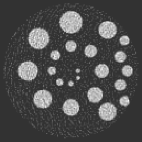
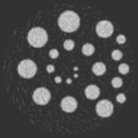
(c)	(d)

Figure 2: Geometry #1: (a) phantom, (b) reconstruction from the accurate projections (c) effect of 15% noise in projections (d) reconstruction from the noisy projections with the additional filter

In order to verify the accuracy and stability of the present algorithm we conducted a series of numerical experiments . In particular, we studied two acquisition geometries (which we will call #1 and #2) corresponding to different values of parameters $x_{\mathit{right}}$ and $z_{\mathit{right}},$ (see Figure 1). In both geometries $R$ and $R_{\gamma}$ are equal to $1$ and $1.3$ respectively. Geometry #1 has $x_{\mathit{right}}$=$z_{\mathit{right}}=1;$ in other words, the ROI is a unit circle. Geometry #2 is defined by values $x_{\mathit{right}}$=$z_{\mathit{right}}=0,$ which corresponds to a half-circle acquisition curve and a half-disk ROI. Both geometries satisfy the visibility condition. In all experiments reconstruction was performed on an equispaced Cartesian $129\times 129$ grid, from simulated projections corresponding to $500$ equispaced detectors, each measuring 129 circular integrals with equispaced radii. (The radial step in the projections coincides with the step of the reconstruction grid under such discretization).

The goal of our first test was to verify the feasibility of the approximation of plane waves by the single layer potentials. We found that the most difficult plane waves to approximate were the ones propagating in the vertical direction. In geometry #1 the method described in Section 3.3 with $K=1.5$ gave approximations accurate up to 4 decimal places or better. In particular, for the plane wave propagating in the vertical direction with the wavelength corresponding to the Nyquist frequency of our $129\times 129$ grid, the maximum pointwise error did not exceed $8\cdot 10^{-6}.$ Similar (although slightly less accurate) results were obtained in the geometry #2.

These accurate approximations of the plane waves lead to very accurate reconstructions of smooth images. For geometry #1 we defined a smooth phantom as follows. First, we introduced a $C_{0}^{8}(\mathbb{R})$ function $h(t)$:

$$h(t)=\left\{\begin{array}[c]{lll}c_{0}\int_{0}^{1-|t|}\sin^{8}(\pi s)ds&,&0\leq|t|\leq 1\\ 0&,&|t|>1\end{array}\right.$$

where constant $c_{0}$ was chosen so that $h(0)=1.$ Function $h(t)$ is even, compactly supported on $[-1,1],$ 8 times continuously differentiable on $\mathbb{R}$ function, with $h(1/2)=1/2.$ We then used this function to construct the 8 times continuously differentiable phantom $f(x)=h\left(\frac{|x-x_{1}|}{r_{1}}\right)+h\left(\frac{|x-x_{2}|}{r_{2}}\right),$ as a sum of two bell-shaped rotationally invariant functions. For geometry #1 we used parameters $x_{1}=(0.3,0.3),x_{2}=(-0.4,0.2),$ $r_{1}=0.55,$ $r_{2}=0.5.$ Reconstruction using the present method (without additional filtration) resulted in maximal point-wise error of $7.3\cdot 10^{-5}.$ Similarly small reconstruction errors were obtained for smooth phantoms in geometry #2. We do not present here the gray scale pictures of these phantoms and the corresponding reconstructed images since they look identically. The experiments with smooth phantoms show that our method indeed reconstructs accurately all the spatial frequencies of the image (including the lower ones) — as opposed to parametrix approximations.

Our next experiment was with discontinuous phantoms. Point-wise accurate reconstructions are not possible with such functions due to the aliasing errors and the Gibbs phenomenon; the goal is to obtain images that appear qualitatively correct, with low noise amplification. As a phantom in geometry #1, we used the sum of the characteristic functions of circles as shown in Figure 2(a). Part (b) of the latter figure demonstrates the image reconstructed from accurate projections. In order to analyze the sensitivity of the method to non-exact measurements we added to the projections white noise with intensity of $15\%$ of the signal (in $L^{2}$ norm); the reconstruction is shown in Figure 2(c). As it is frequently done in tomography, in order to reduce the effects of noise one can apply a low-pass filter on step 4 of the algorithm. Part (d) demonstrates the effect of such additional filtration, with filter $\eta(\xi)=\cos(\frac{\pi}{2}|\xi|/\lambda_{\mathit{Nyquist}})$, where $\lambda_{\mathit{Nyquist}}$ is the Nyquist frequency of the reconstruction grid.

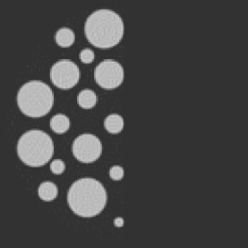
(a)	(b)
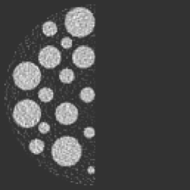
(c)	(d)

Figure 3: Geometry #2: (a) phantom, (b) reconstruction from the accurate projections (c) effect of 15% noise in projections (d) reconstruction from the noisy projections with the additional filter

Quite similar results were obtained in geometry #2. As a phantom we used again a sum of the characteristic functions of circles supported within the ROI (the left half of the unit disk)), as shown in Figure 3(a). Parts (b), (c), and (d) of that figure demonstrate, respectively, reconstruction results from the accurate projections, noisy projections, and reconstruction from noisy projections with additional filtration (using the same filter as in the previous example).

In order to compare stability of our algorithm to that of the classical FBP, we have reconstructed the two phantoms (shown in Figure 2(a) and Figure 3(a)) using the latter method, from a similar number of the standard Radon projections with the same level of noise (not shown here). The general quality and the level of noise in the reconstructions was quite close to those of the images obtained by the present method.

From the practical point of view it is interesting to know how the reconstruction is affected by acoustic sources located outside of the ROI. It is known that, with the exception of the methods based on expansion in the eigenvalues of the Dirichlet Laplacian on a closed domain [2, 19], all the other exact reconstruction techniques will produce incorrect results in the presence of such sources (see [1, 16, 13] for further discussion of this phenomenon). In our case, such sources will be present if the electromagnetic wave impinges on the parts of the patient’s body located outside the ROI. In other to model this situation in geometry #2 we used the previously used phantom supported within the unit disk, as shown in Figure 2(a). The result of the reconstruction in the absence of noise is shown in Figure 4(a); part (b) demonstrates the effect of 15% noise and the additional filtration.

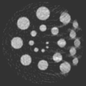
(a)	(b)

Figure 4: Geometry #2: (a) reconstruction with some sources outside of the ROI (compare to Figure 2(a)) (b) the same with 15% noise in the projections and with the additional filter

One can notice in this figure that the parts of the source located outside ROI are not reconstructed correctly (not unexpectedly). Nevertheless, by covering the right half of the image, it is easy to see that the reconstruction within the ROI is very little (if at all) affected by the presence of additional sources outside the region. Interestingly, in the right half of the image (outside ROI), the ”visible” material interfaces are reconstructed quite well, while the ”invisible” ones (such that the normal does not intersect the measuring surface) are noticeably smeared.

In accordance with the theoretical operation count, step #1 turned out to be the most expensive part of the algorithm; in the experiments described in this section the computation of the densities took several hours. However, this step needs to be performed only once for a given geometry. On consecutive runs of the reconstruction program, once the pre-computed densities had been read from the hard drive, the algorithm took a fraction of a second to complete. The time required to read the densities was about 4 seconds. If our method were to be used to process the data obtained by an acquisition scheme with linear detectors (which requires the inversion of a set of 2-D problems), the densities would need to be read only once, and each of the 2-D problems would be inverted in a fraction of second.

5 Concluding remarks

We have presented an efficient reconstruction algorithm applicable to problems of thermoacoustic tomography with the detectors lying on an open curve. The method is based on $L^{2}$ approximations of plane waves by certain single layer potentials; we have proven that such approximations are possible if the measurement curve is an open circular arch. We have also verified numerically that, for the truncated circular geometry satisfying the ”visibility” condition one can obtain very accurate approximations with bounded densities, which, in turn, leads to stable image reconstructions.

In conclusion, we would like to add several remarks:

• The theorem we have presented does not restrict the shape of the ROI; it can be arbitrary. Of course, for stable reconstruction the combination of the ROI and the acquisition surface should satisfy the ”visibility” condition.

• In the proof of the theorem we used the fact that if the solution of the Helmholtz equation vanishes on a circular arch, it must vanish on the whole circle, and, therefore, in the exterior of the disk. A similar statement is also true if the acquisition curve is a part of any closed analytic curve, and the theorem extends to such configurations. The theorem also remains valid if the measurement curve is a continuous non-analytic curve.

• In order to use this approach with non-circular acquisition curves, the regularization technique we presented may require some modifications, since it is based on the comparison with the full-circle case.

• The technique we propose can also be used in 3-D, for image reconstruction from the detectors lying on an open surface. Compliance with the ”visibility” condition is, again, necessary for a stable reconstruction in this case. We anticipate that the pre-computation of the densities may become quite time-consuming in 3-D, due to the increased dimensionality of the problem. The development of a fast algorithm for this part of our method is required to make this approach practical (in 3-D). This will be the object of our future research.

6 Acknowledgements

The author would like to thank Professor P. Kuchment for fruitful discussions and numerous helpful suggestions.

This work was partially supported in part by the NSF/DMS grant NSF-0312292 and by the DOE grant DE-FG02-03ER25577.

References

- [1] Agranovsky M, Kuchment P and Kunyansky L 2008 On reconstruction formulas and algorithms for the thermoacoustic and photoacoustic tomography, to appear in Photoacoustic Imaging and Spectroscopy, CRC Press.
- [2] Agranovsky M and Kuchment P 2007 Uniqueness of reconstruction and an inversion procedure for thermoacoustic and photoacoustic tomography with variable sound speed Inverse Problems 23, 2089-2102
- [3] Agranovsky M and Quinto E T 1996 Injectivity sets for the Radon transform over circles and complete systems of radial functions Journal of Functional Analysis 139 383–414
- [4] Anastasio M, Zhang J, Pan X, Zou Y, Ku G, Wang LV 2005 Half-Time Image Reconstruction in Thermoacoustic Tomography IEEE Trans. Med Imag 24(2) 199-210
- [5] Beylkin G 1984 The inversion problem and applications of the generalized Radon transform Communications on Pure and Applied Mathematics 37(5) 579-599
- [6] Burgholzer P, Hofer C, Paltauf G, Haltmeier M and Scherzer O 2005 Thermoacoustic tomography with integrating area and line detectors IEEE Trans. Ultrason. Ferroelect. Freq. Contr. 52 1577-83
- [7] Burgholzer P, Grün H, Bauer-Marschallinger J, Haltmeier M and Paltauf G 2007 Temporal back projection algorithms for photoacoustic tomography with integrating line detectors Inverse Problems 23 S65–S80
- [8] Burgholzer, P., Matt, G., Haltmeier, M. & Patlauf, G. 2007. Exact and approximate imaging methods for photoacoustic tomography using an arbitrary detection surface. Phys. Rev. E 75 046706
- [9] Colton D and Kress R 1992 Inverse acoustic and electromagnetic scattering theory, Springer-Verlag.
- [10] Finch D, Haltmeier M and Rakesh 2007. Inversion of spherical means and the wave equation in even dimensions. SIAM J. Appl. Math. 68(2) 392-412
- [11] Finch D and Rakesh 2008 Recovering a function from its spherical mean values in two and three dimensions, to appear in Photoacoustic Imaging and Spectroscopy, CRC Press.
- [12] Finch, D, Patch S and Rakesh 2004 Determining a function from its mean values over a family of spheres SIAM J. Math. Anal. 35(5) 1213-40
- [13] Hristova Y, Kuchment P and Nguyen L On reconstruction and time reversal in thermoacoustic tomography in homogeneous and non-homogeneous acoustic media, to appear in Inverse Problems.
- [14] Kak A C and Slaney M 1988 Principles of Computerized Tomographic Imaging, IEEE
- [15] Kruger R A, Liu P, Fang Y R, and Appledorn C R 1995. Photoacoustic ultrasound (PAUS) reconstruction tomography Med. Phys. 22 1605-09
- [16] Kuchment P and Kunyansky L 2008 Mathematics of thermoacoustic tomography, in ”A Survey in Mathematics for Industry” European Journal of Applied Mathematics 19 191-224
- [17] Kuchment P, Lancaster K and Mogilevskaya L 1995 On the local tomography Inverse Problems 11 571-89
- [18] Kunyansky L 2007 Explicit inversion formulae for the spherical mean Radon transform Inverse Problems 23 373-83
- [19] Kunyansky L 2007 A series solution and a fast algorithm for the inversion of the spherical mean Radon transform. Inverse Problems 23 S11-S20
- [20] Louis A K and Quinto E T 2000 Local tomographic methods in Sonar. In Surveys on solution methods for inverse problems, Springer, Vienna, 147-154
- [21] Natterer F 1986 The Mathematics of Computerized Tomography, Wiley.
- [22] Norton S J 1980 Reconstruction of a two-dimensional reflecting medium over a circular domain: exact solution J. Acoust. Soc. Am. 67 1266-73
- [23] Norton S J and Linzer M 1981 Ultrasonic reflectivity imaging in three dimensions: exact inverse scattering solutions for plane, cylindrical, and spherical apertures IEEE Trans. on Biomed. Eng. 28 200-202
- [24] Quinto E T 1993 Singularities of the X-ray transform and limited data tomography in and SIAM J. Math. Anal. 24 1215-1225
- [25] Palamodov V P 2004 Reconstructive Integral Geometry, Birkhauser.
- [26] Palamodov V P 2000 Reconstruction from limited data of arc means. J. Fourier Anal. Appl. 6(1) 25-42
- [27] Palamodov V P 2007 Remarks on the general Funk-Radon transform and thermoacoustic tomography, arXiv:math/0701204
- [28] Paltauf G, Nuster R, Haltmeier M and Burgholzer P 2007 Experimental evaluation of reconstruction algorithms for limited view photoacoustic tomography with line detectors Inverse Problems 23 S81-S94
- [29] Paltauf G, Nuster R, Haltmeier M and Burgholzer P 2007 Photoacoustic tomography using a Mach–Zehnder interferometer as acoustic line detector Appl. Opt. 46 3352-8
- [30] Paltauf G, Viator J A, Prahl S A, Jacques S L 2002 Iterative reconstruction algorithm for optoacoustic imaging J. Acoust. Soc. Am 112(4) 1536-1544
- [31] Pan X., Zou Y, Anastasio M 2003 Data Redundancy and Reduced-Scan Reconstruction in Reflectivity Tomography IEEE Trans Imag Processing 12(7) 784-795
- [32] Patch S 2008 Photoacoustic or thermoacoustic tomography - consistency conditions and the partial scan problem, to appear in Photoacoustic Imaging and Spectroscopy, CRC Press.
- [33] Popov D A and Sushko D V 2002 A parametrix for the problem of optical-acoustic tomography Dokl. Math. 65(1) 19-21
- [34] Popov D A and Sushko D V 2004 Image restoration in optical-acoustic tomography. Problems of Information Transmission 40(3) 254-278
- [35] Watson G N 1944 A treatise on the theory of Bessel functions 2d ed. Cambridge University Press.
- [36] Xu M and Wang L V 2006 Photoacoustic imaging in biomedicine Review of Sci Instr 77(4) 041101
- [37] Xu M and Wang L V 2006 Universal back-projection algorithm for photoacoustic computed tomography Phys Review E 71(1) 016706
- [38] Xu Y, Wang L, Ambartsoumian G and Kuchment P 2004 Reconstructions in limited view thermoacoustic tomography Medical Physics 31 724-33
- [39] Xu Y, Wang L, Ambartsoumian G and Kuchment P 2008 Limited view thermoacoustic tomography, to appear in Photoacoustic imaging and spectroscopy, CRC Press.