Collective Phase Sensitivity

Abstract

The collective phase response to a macroscopic external perturbation of a population of interacting nonlinear elements exhibiting collective oscillations is formulated for the case of globally-coupled oscillators. The macroscopic phase sensitivity is derived from the microscopic phase sensitivity of the constituent oscillators by a two-step phase reduction. We apply this result to quantify the stability of the macroscopic common-noise induced synchronization of two uncoupled populations of oscillators undergoing coherent collective oscillations.

Nature possesses various examples of systems composed of many nonlinear elements in which, through mutual interactions, coherent collective dynamics emerges Ref:Winfree01 ; Ref:Kuramoto84 ; Ref:Pikovsky01 ; Ref:Manrubia04 ; Ref:Izhikevich07 ; Ref:Brunel99 ; Ref:Strogatz00 ; Ref:Acebron05 ; Ref:Okuda91 ; Ref:Montbrio04 ; Ref:Hudson05 ; Ref:Kiss ; Ref:Ukai07 . The collective dynamics of the population is generally not a simple superposition of the microscopic dynamics of the constituent elements; due to nonlinearities, it can differ qualitatively. Understanding how the microscopic properties give rise to the macroscopic collective properties of the system, and formulating the theory in a simple closed form at the macroscopic level is a fundamental problem in nonlinear dynamics.

If the population undergoes a stable macroscopic limit-cycle oscillation, it can most simply be described by a single macroscopic phase variable. By knowing the collective phase response of the macroscopic oscillation with respect to external perturbations, we can describe the dynamics of the population by the phase picture, much like for single microscopic oscillators Ref:Winfree01 ; Ref:Kuramoto84 ; Ref:Pikovsky01 ; Ref:Manrubia04 ; Ref:Izhikevich07 . The collective phase response can be measured operatively by macroscopically applying an external perturbation to the population without recourse to the microscopic details Ref:Winfree01 ; Ref:Hudson05 ; Ref:Ukai07 . However, to understand how the microscopic dynamics of the constituent elements and their mutual interactions conspire to become a macroscopic phase response, it is necessarily to develop a statistical mechanical approach.

In this paper, we formulate this problem for globally-coupled oscillators as a simple model of macroscopic populations exhibiting collective oscillations. Global coupling is the simplest form of mutual interactions, which is both conceptually and practically important because it serves as a starting point for theoretical analysis of various network-coupled dynamical systems and because it is realized in experimental systems  Ref:Winfree01 ; Ref:Kuramoto84 ; Ref:Pikovsky01 ; Ref:Manrubia04 ; Ref:Acebron05 ; Ref:Kiss . We quantitatively derive the collective phase sensitivity, which is the linear response coefficient of the macroscopic collective phase response, from the microscopic phase sensitivity of the constituent oscillators using a two-step phase-reduction on the micro- and macroscopic scales.

The collective phase sensitivity is a fundamental quantity characterizing the response of a macroscopic limit-cycle oscillation to weak external perturbations. As one application, we analyze macroscopic common-noise induced synchronization of the collective oscillations between two uncoupled populations. Though not treated in this paper, the entrainment of a population to external forcing or synchronization between populations can also easily be analyzed using the collective phase sensitivity.

Let us give a general definition of the collective phase sensitivity first. We consider a population of globally-coupled noisy identical limit-cycle oscillators collectively exhibiting stable macroscopic limit-cycle oscillations. We assume that the effect of coupling, noise, and perturbations is sufficiently weak, so that the orbit of each microscopic oscillator is always near its limit cycle. We can then describe each oscillator by the phase $\phi$, and the whole population by a single-oscillator phase probability density function (PDF) $P(\phi,t)$ of the constituent oscillators. As the population undergoes limit-cycle oscillations, $P(\phi,t)$ is given in the form of a rotating wave packet of constant shape (see Figs. 1 and 3),

$$P(\phi,t)=f\left(\phi-\Phi(t)\right),\;\;\;\Phi(t)=\Omega t+\Theta,$$ (1)

where $f(\phi)$ represents the wave packet, $\Phi(t)$ the collective phase of the population (location of the wave packet) at time $t$, $\Omega$ the frequency of the collective oscillation, and $\Theta$ the initial collective phase. We assume $\phi\in[-\pi,\pi]$ and impose a periodic boundary condition $f(\phi+2\pi)=f(\phi)$.

At the instant that the collective phase is $\Phi_{0}$, we apply a macroscopic perturbation of magnitude and direction ${\bm{s}}$ that acts uniformly on all oscillators. The shape of $P(\phi,t)$ transiently deforms, but due to the stability of the collective oscillations, eventually settles into its stationary shape, Eq. (1). We denote the perturbed PDF after a sufficiently long time $t_{0}$ as $P_{1}(\phi,t+t_{0})=f\left(\phi-\Phi_{1}(\Phi_{0},{\bm{s}},t_{0})\right)$, and the unperturbed PDF after time $t_{0}$ as $P_{2}(\phi,t+t_{0})=f\left(\phi-\Phi_{2}(\Phi_{0},t_{0})\right)$, where $\Phi_{2}=\Phi_{0}+\Omega t_{0}$. The collective phase response function $G(\Phi_{0};{\bm{s}})$ is defined as the asymptotic difference of $\Phi_{1}(\Phi_{0},{\bm{s}},t_{0})$ and $\Phi_{2}(\Phi_{0},t_{0})$: $G(\Phi_{0};{\bm{s}})=\lim_{t_{0}\to\infty}\left[\Phi_{1}(\Phi_{0},{\bm{s}},t_{0})-\Phi_{2}(\Phi_{0},t_{0})\right]$ Ref:Winfree01 . This is in general a function of $\Phi_{0}$ and ${\bm{s}}$. When the impulse magnitude $|{\bm{s}}|$ is small enough, the collective phase response function is proportional to ${\bm{s}}$, and is given by $G(\Phi_{0};{\bm{s}})=\bm{\zeta}(\Phi_{0})\cdot{\bm{s}}$, where $\bm{\zeta}(\Phi_{0})$ is the collective phase sensitivity Ref:Kuramoto84 .

We consider globally-coupled oscillators described by the following Langevin equation:

$$\dot{\bm{X}}_{j}(t)={\bm{F}}({\bm{X}}_{j}(t))+\frac{1}{N}\sum_{k=1}^{N}{\bm{V}}({\bm{X}}_{k}(t))+\sqrt{2D_{0}}\,{\bm{\eta}}_{j}(t)+{\bm{s}}(t),$$ (2)

for $j=1,\cdots,N$, where ${\bm{X}}_{j}$ is the state of the $j$th oscillator, ${\bm{F}}({\bm{X}})$ the dynamics of a single oscillator, ${\bm{V}}({\bm{X}})$ the contribution from each oscillator to the mean field, $D_{0}$ the noise intensity, ${\bm{\eta}}_{j}(t)$ an independent zero-mean Gaussian white noise of unit intensity, which satisfies $\langle{\bm{\eta}}_{j}(t){\bm{\eta}}_{k}(t^{\prime})\rangle={\bf I}\delta_{j,k}\delta(t-t^{\prime})$ where ${\bf I}$ is the unit matrix, and ${\bm{s}}(t)$ the macroscopic external perturbation common to all oscillators. When isolated, each oscillator has a stable limit-cycle ${\bm{X}}_{0}(t+T)={\bm{X}}_{0}(t)$ with period $T=2\pi/\omega$. We define a phase $\phi({\bm{X}})\in[-\pi,\pi]$ around the limit cycle, which increases with a constant natural frequency $\omega$ Ref:Kuramoto84 . We assume that the effect of coupling, noise, and perturbation is sufficiently weak.

To derive a dynamical equation for the single-oscillator phase PDF of our system, we perform the first, microscopic phase reduction of Eq. (2). Using the microscopic phase sensitivity of each oscillator, ${\bm{Z}}(\phi)=\nabla_{\bm{X}}\phi|_{{\bm{X}}={\bm{X}}_{0}(\phi)}$ Ref:Kuramoto84 , the dynamics of the system can be reduced to the following Langevin phase equation:

$$\dot{\phi}_{j}(t)=\omega+\frac{1}{N}\sum_{k=1}^{N}{\bm{Z}}(\phi_{j})\cdot{\bm{V}}({\bm{X}}_{0}(\phi_{k}))+\sqrt{2D_{0}}\,{\bm{Z}}(\phi_{j})\cdot{\bm{\eta}}_{j}(t)+\xi(\phi_{j},t),$$ (3)

where the effect of the perturbation is given by $\xi(\phi_{j},t)={\bm{Z}}(\phi_{j})\cdot{\bm{s}}(t)$. From this equation, after averaging and taking the limit as $N\to\infty$ (see Ref:Kuramoto84 ; Ref:Kawamura07 for details), we obtain the nonlinear Fokker-Planck equation (FPE) for the single-oscillator phase PDF $P(\phi,t)$,

$$\frac{\partial}{\partial t}P(\phi,t) =-\frac{\partial}{\partial\phi}\left\{\left[\omega+\int_{-\pi}^{\pi}\Gamma(\phi-\phi^{\prime})P(\phi^{\prime},t)d\phi^{\prime}+\xi(\phi,t)\right]P(\phi,t)\right\}+D\frac{\partial^{2}}{\partial\phi^{2}}P(\phi,t),$$ (4)

where the phase coupling function is given by $\Gamma(\phi-\phi^{\prime})=(1/2\pi)\int_{-\pi}^{\pi}{\bm{Z}}(\phi+\psi)\cdot{\bm{V}}(\phi^{\prime}+\psi)d\psi$, and the diffusion coefficient by $D=(D_{0}/2\pi)\int_{-\pi}^{\pi}{\bm{Z}}(\psi)\cdot{\bm{Z}}(\psi)d\psi$. The external perturbation $\xi(\phi,t)$ in the drift term is not averaged, but kept as a time-dependent term.

To realize stable macroscopic oscillations, we assume that the coupling function $\Gamma(\phi)$ is unimodal and satisfies the in-phase (attractive) condition $d\Gamma(\phi)/d\phi|_{\phi=0}<0$ Ref:Kuramoto84 . When there is no external perturbation ($\xi(\phi,t)\equiv 0$), the solution of Eq. (4) is given by a rotating wave packet of the form Eq. (1), which behaves as follows: In the absence of independent noise ($D_{0}=0$), the oscillators are completely synchronized, so that $P(\phi,t)$ is delta-peaked. As $D_{0}$ is increased, $P(\phi,t)$ takes on a finite width while rotating at a constant speed. As $D_{0}$ increases past a critical value $D_{\rm c}$, the collective oscillation disappears, and $P(\phi,t)\equiv 1/2\pi$. For the following analysis, we take $0<D_{0}<D_{\rm c}$.

We now derive the collective phase sensitivity $\bm{\zeta}(\Phi)$ from the microscopic phase sensitivity ${\bm{Z}}(\phi)$ by seeking a closed equation for the collective phase $\Phi(t)$. This is performed by the second, macroscopic phase reduction, similarly to the derivation of wavefront dynamics for oscillatory media Ref:Kuramoto84 . Our treatment here is a generalization of Ref:Kawamura07 for nonlocally-coupled noisy oscillators. Let us ignore the perturbation for the moment ($\xi(\phi,t)\equiv 0$). Introducing a corotating phase with the wave packet, $\theta=\phi-\Phi(t)=\phi-\Omega t-\Theta$, the solution of Eq. (4), $P(\phi,t)=f(\theta)$, satisfies $D(d^{2}/d\theta^{2})f(\theta)-(d/d\theta)\left\{\left[(\omega-\Omega)+\int_{-\pi}^{\pi}\Gamma(\theta-\theta^{\prime})f(\theta^{\prime})d\theta^{\prime}\right]f(\theta)\right\}=0$. Small deviations $u(\theta)$ from this unperturbed wave packet $f(\theta)$ obey a linearized equation $\partial_{t}u(\theta,t)=\hat{L}u(\theta,t)$, where the linear operator $\hat{L}$ is given by

$$\hat{L}u(\theta)=D\frac{d^{2}}{d\theta^{2}}u(\theta)-\frac{d}{d\theta}\left\{\left[(\omega-\Omega)+\int_{-\pi}^{\pi}\Gamma(\theta-\theta^{\prime})f(\theta^{\prime})d\theta^{\prime}\right]u(\theta)\right\}-\frac{d}{d\theta}\left\{f(\theta)\int_{-\pi}^{\pi}\Gamma(\theta-\theta^{\prime})u(\theta^{\prime})d\theta^{\prime}\right\}.$$ (5)

Defining the inner product as $[u^{\ast}(\theta),u(\theta)]=\int_{-\pi}^{\pi}u^{\ast}(\theta)u(\theta)d\theta$, we introduce an adjoint operator $\hat{L}^{\ast}$ of $\hat{L}$ by $[u^{\ast}(\theta),\hat{L}u(\theta)]=[\hat{L}^{\ast}u^{\ast}(\theta),u(\theta)]$. In the calculation below, we only need zero eigenfunctions $u_{0}(\theta)$ of $\hat{L}$ and $u_{0}^{\ast}(\theta)$ of $\hat{L}^{\ast}$, which we normalize as $[u^{\ast}_{0}(\theta),u_{0}(\theta)]=1$. It is easy to check that $u_{0}(\theta)$ can be chosen as $u_{0}(\theta)=df(\theta)/d\theta$, reflecting the translational symmetry of Eq. (4) Ref:Kuramoto84 ; Ref:Kawamura07 .

We now incorporate the effect of perturbation, $\xi(\phi,t)$. To obtain a closed equation for $\Phi(t)$, we assume that the solution of Eq. (4) is still given in the form of Eq. (1), ignoring its slight deformation at the lowest order. Instead, we allow the constant $\Theta$ in Eq. (1) to vary slowly with time as $\Theta(t)$. Plugging $P(\phi,t)=f(\theta(t))=f(\phi-\Omega t-\Theta(t))$ into Eq. (4), we obtain $u_{0}(\theta)\dot{\Theta}(t)=(d/d\theta)\left\{\xi(\theta+\Omega t+\Theta(t),t)f(\theta)\right\}$. Taking the inner product with $u_{0}^{\ast}(\theta)$ on both sides yields $\dot{\Theta}(t)=\int_{-\pi}^{\pi}u_{0}^{\ast}(\theta)(d/d\theta)\left\{\xi(\theta+\Omega t+\Theta(t),t)f(\theta)\right\}d\theta.$ Noting that $\xi(\theta+\Omega t+\Theta(t),t)=\xi(\theta+\Phi(t),t)={\bm{Z}}(\theta+\Phi(t))\cdot{\bm{s}}(t)$, we arrive at the macroscopic phase equation obeyed by $\Phi(t)$,

$$\dot{\Phi}(t)=\Omega+{\bm{\zeta}}(\Phi(t))\cdot{\bm{s}}(t),$$ (6)

where the collective phase sensitivity is given by

$${\bm{\zeta}}(\Phi) =\int_{-\pi}^{\pi}\left(-\frac{du_{0}^{\ast}(\theta)}{d\theta}f(\theta)\right){\bm{Z}}(\theta+\Phi)d\theta.$$ (7)

Thus, ${\bm{\zeta}}(\Phi)$ is expressed as a convolution of the microscopic phase sensitivity ${\bm{Z}}(\theta)$ with a kernel $-u_{0}^{\ast}(\theta)^{\prime}f(\theta)$. Note the kernel is not merely the PDF $f(\theta)$ as we would naively expect.

Now let us illustrate our results with an example of $N$ noisy globally-coupled Stuart-Landau (SL) oscillators described by the following Langevin equation Ref:Kuramoto84 ; Ref:Kawamura07 : $\dot{W}_{j}(t)=(1+i\omega_{0})W_{j}-(1+i\beta)|W_{j}|^{2}W_{j}+(K/N)\sum_{k=1}^{N}W_{k}+\sqrt{2D_{0}}\,\eta_{j}(t)+s(t)$. Here, the complex amplitude $W_{j}=W^{\rm R}_{j}+iW^{\rm I}_{j}$ (${\rm R}$ and ${\rm I}$ express real and imaginary components, respectively) describes the state of the $j$th oscillator (i.e. ${\bm{X}}_{j}=(W^{\rm R}_{j},W^{\rm I}_{j})$), $\omega_{0}$ and $\beta$ are oscillator parameters, $K$ the coupling strength, $s(t)=s^{\rm R}(t)+is^{\rm I}(t)$ the macroscopic complex perturbation, $D_{0}$ the noise intensity, and $\eta_{j}(t)=\eta^{\rm R}_{j}(t)+i\eta^{\rm I}_{j}(t)$ the independent complex Gaussian white noise of zero mean and unit intensity which satisfies $\langle\eta^{\rm R}_{j}(t)\eta^{\rm R}_{k}(t^{\prime})\rangle=\langle\eta^{\rm I}_{j}(t)\eta^{\rm I}_{k}(t^{\prime})\rangle=\delta_{j,k}\delta(t-t^{\prime})$ and $\langle\eta^{\rm R}_{j}(t)\eta^{\rm I}_{k}(t^{\prime})\rangle=0$. The phase $\phi$ is defined on the complex plane as $\phi=\arg W-\beta\ln|W|$, which grows constantly with a natural frequency $\omega=\omega_{0}-\beta$ in the absence of coupling and other external effects. The microscopic phase sensitivity has both real and imaginary parts, given analytically as ${\bm{Z}}(\phi)=(Z^{\rm R}(\phi),Z^{\rm I}(\phi))=(-\sin\phi-\beta\cos\phi,\,\cos\phi-\beta\sin\phi)$, and the phase coupling function is given by $\Gamma(\phi-\phi^{\prime})=-K\sqrt{1+\beta^{2}}\sin(\phi-\phi^{\prime}+\alpha),\,\alpha=\arg(1+i\beta)$ Ref:Kuramoto84 ; Ref:Kawamura07 . We use the complex order parameter $A(t)=R(t)e^{i\tilde{\Phi}(t)}=(1/N)\sum_{k=1}^{N}e^{i\phi_{k}(t)}\simeq\int_{-\pi}^{\pi}e^{i\phi}f(\phi-\Phi(t))d\phi$ to quantify the collective oscillation, whose modulus $R(t)$ serves as a measure of the coherence Ref:Kuramoto84 ; Ref:Kawamura07 . By choosing $f(\phi)$ so that $\int_{-\pi}^{\pi}e^{i\phi}f(\phi)d\phi$ is positive and real, and taking the initial collective phase as $\Theta=0$, namely, $P(\phi,0)\equiv f(\phi)$, the phase $\tilde{\Phi}(t)$ of the order parameter $A(t)$ matches the collective phase $\Phi(t)$ defined in Eq. (1).

Figure 1 shows the stationary PDF $f(\phi)$, the zero eigenfunctions $u_{0}(\phi)$ and $u_{0}^{\ast}(\phi)$, and the kernel $-u_{0}^{\ast}(\phi)^{\prime}f(\phi)$, obtained by numerically solving Eq. (4). The parameters $\omega_{0}=2$, $\beta=1$, $K=0.05$ are fixed, while the noise intensity is varied as $D_{0}=0.009$, $0.011$, $0.012$. As $D_{0}$ approaches the critical value $D_{\rm c}=0.0125$  Ref:Kuramoto84 ; Ref:Kawamura07 , $f(\phi)$ becomes flat, while the amplitudes of $u_{0}^{\ast}(\phi)$ and the kernel $-u_{0}^{\ast}(\phi)^{\prime}f(\phi)$ increase. Figure 2(a) shows the real part of the collective phase sensitivity $\zeta^{\rm R}(\Phi)$ calculated using the results shown in Fig. 1 (the imaginary part is simply given by $\zeta^{\rm I}(\Phi)=\zeta^{\rm R}(\Phi-\pi/2)$ due to symmetry of the SL oscillator). For comparison, we show the microscopic phase sensitivity, $Z^{\rm R}(\phi)$ with $\phi=\Phi$, which corresponds to the $D_{0}\to 0$ limit. For $D_{0}>0$, $\zeta^{\rm R}(\Phi)$ is different from $Z^{\rm R}(\phi)$ due to distributed individual phases. As $D_{0}\to D_{\rm c}$, $\zeta^{\rm R}(\Phi)$ diverges as $(D_{\rm c}-D_{0})^{-1/2}$ footnote2 . Figure 2(b) compares the theoretical $\zeta^{\rm R}(\Phi)$ at $D_{0}=0.009$ with those directly measured by adding sufficiently weak impulses ($|s|=0.001$) to the nonlinear FPE (4) and to the Langevin equation (2) with $N=10,000$ oscillators footnote3 . The results of the nonlinear FPE corresponding to the limit $N\to\infty$ agrees well with the theory footnote4 . The results of the Langevin simulation show a wide distribution of the values because $N$ is necessarily finite, though the piecewise average value shows reasonable agreement with the theory footnote5 .

As an application of the collective phase sensitivity, we analyze the stability of the synchronized state of two uncoupled populations of collectively oscillating, globally-coupled SL oscillators due to a macroscopic common noise. Consider two uncoupled macroscopic phase oscillators driven by a common, weak Gaussian noise ${\bm{s}}(t)$: $\dot{\Phi}^{(\sigma)}(t)=\Omega+{\bm{\zeta}}(\Phi^{(\sigma)}(t))\cdot{\bm{s}}(t)\ (\sigma=1,2)$, where the noise correlation is given by $\langle\bm{s}(t)\bm{s}(0)\rangle={\bf I}C(t)$. In Ref:Teramae04 , it is shown that a weak common Gaussian noise will cause synchronization of uncoupled oscillators, and the Lyapunov exponent that quantifies the growth rate of an infinitesimal phase difference is given by $\Lambda=(1/2\pi)\int_{0}^{\infty}dt\,C(t)\int_{-\pi}^{\pi}d\Phi\,{\bm{\zeta}}^{\prime\prime}(\Phi)\cdot{\bm{\zeta}}(\Phi-\Omega t)$, where $\Lambda\leq 0$ always holds. For the globally-coupled SL oscillators, the perturbation ${\bm{s}}(t)$ has real and imaginary components. We use the Ornstein-Uhlenbeck process Ref:Gardiner97 , $\dot{z}(t)=-z/\tau+\chi(t)/\tau$ with $\chi(t)$ a zero-mean Gaussian white noise of unit intensity, to create colored Gaussian noises $z^{\rm R,I}(t)$ with the correlation time $\tau$, and put ${\bm{s}}(t)=\sqrt{2S}(z^{\rm R}(t),\,z^{\rm I}(t))$ where $S$ controls the intensity of common noise. The correlation function is given as $C(t)=S\exp(-|t|/\tau)/\tau$.

Figure 3 shows the results for two uncoupled populations of $N=1000$ globally-coupled SL oscillators receiving macroscopic common Gaussian noise of intensity $S=0.001$ with correlation times $\tau=1.0$, $\tau=0.5$, and $\tau\to 0$ (white limit). Other parameters are $\omega_{0}=2$, $\beta=1$, $K=0.05$, and $D_{0}=0.007$. Figures 3(a) and 3(d) show the time evolution of the real part of the order parameter $A(t)$ of the two populations obtained by the Langevin simulation. At time $t=0$, the two are not synchronized, but by $t=600$, they show near-complete synchronization, demonstrating that macroscopic common noise can cause the collective oscillations of two uncoupled populations to synchronize. We stress that this is purely a macroscopic phenomenon of the collective phase becoming entrained; the oscillators in the two populations never become individually synchronized. Figures 3(b) and 3(e) show the distributions of the states $\{W_{j}\}$ of the microscopic oscillators on a complex plane at $t=0$ and $t=600$, and Figs. 3(c) and 3(f) show the corresponding histogram of the phases $\{\phi_{j}\}$. At $t=0$, the distributions of oscillators only slightly overlap, while by $t=600$, they overlap considerably. Figure 3(g) compares the Lyapunov exponent $\Lambda$ as measured from the Langevin simulation, averaged over $1500$ sample paths, with the theoretical results. Despite the relatively large fluctuations shown by the collective oscillations, we see that $\Lambda$ shows good agreement with theory. As $D_{0}$ approaches the critical value $D_{\rm c}$, the amplitude of the collective phase sensitivity ${\bm{\zeta}}(\Phi)$ increases, so $\Lambda$ takes on ever larger, negative values. However, near the critical point, the phase response becomes strongly nonlinear, so that the numerical results diverge from the linear theory based on the collective phase sensitivity.

In summary, we derived the macroscopic collective phase sensitivity from the microscopic phase sensitivity for a population of globally-coupled oscillators, and analyzed the common-noise induced synchronization of two such populations. By virtue of the assumption that the constituent oscillators are only weakly perturbed, we could utilize the phase reduction method to construct a general framework for the collective phase sensitivity, which may bring a new perspective to the existing body of research on coupled collective oscillations Ref:Okuda91 ; Ref:Montbrio04 ; Ref:Hudson05 . Since we treated the SL oscillators as an example, the resulting collective phase sensitivity was always sinusoidal, with only a change in amplitude. For other types of oscillators, the shape of the collective phase sensitivity may differ significantly than that of its constituent oscillators. Furthermore, the collective phase response to strong macroscopic perturbations should prove to be even more intriguing, though our present framework based on phase reduction is not applicable in this scenario. More detailed and generalized analysis will be reported in the near future.

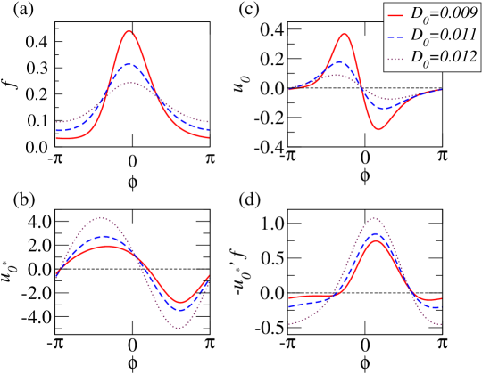
Figure 1: (color online). Globally-coupled SL model. (a) Stationary PDF $f(\phi)$, (b) zero eigenfunction $u_{0}^{\ast}(\phi)$ of $\hat{L}^{\ast}$, (c) zero eigenfunction $u_{0}(\phi)$ of $\hat{L}$, and (d) kernel $-u_{0}^{\ast}(\phi)^{\prime}f(\phi)$.

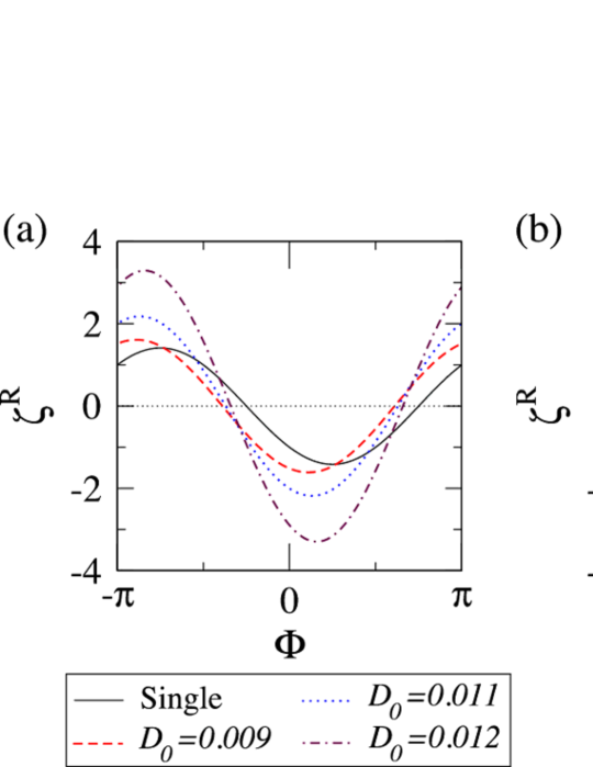
Figure 2: (color online). Collective phase sensitivity of globally-coupled SL model. (a) Theoretical curves of $\zeta^{\rm R}(\Phi)$. Single-oscillator phase sensitivity $Z^{\rm R}(\phi)$ is also shown with $\phi=\Phi$. (b) $\zeta^{\rm R}(\Phi)$, found from theory and from numerical simulations of nonlinear FPE and Langevin equation (LE). For the LE simulation, individual raw responses are shown as dots and piecewise mean values (25 bins) are shown as a solid line.

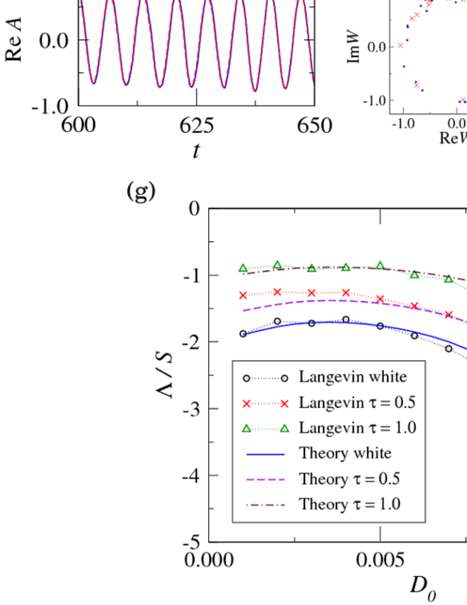
Figure 3: (color online). Common-noise induced synchronization of globally-coupled SL populations. Time evolution of the real part of $A(t)$ from (a) $t=0$ and (d) $t=600$. Snapshots of $\{W_{j}\}$ at (b) $t=0$ and (e) $t=600$ (1/5 of population shown). PDF of phase at (c) $t=0$ and (f) $t=600$. (g) Comparison between Lyapunov exponent $\Lambda$, found from theory and Langevin simulation.

References

- (1) A. T. Winfree, The Geometry of Biological Time (Springer, Second Edition, New York, 2001).
- (2) Y. Kuramoto, Chemical Oscillations, Waves, and Turbulence (Springer, New York, 1984).
- (3) A. Pikovsky, M. Rosenblum, and J. Kurths, Synchronization (Cambridge University Press, Cambridge, 2001).
- (4) S. C. Manrubia, A. S. Mikhailov, and D. H. Zanette, Emergence of Dynamical Order (World Scientific, Singapore, 2004).
- (5) E. M. Izhikevich, Dynamical Systems in Neuroscience (MIT Press, Cambridge, MA, 2007).
- (6) N. Brunel and V. Hakim, Neural Comput. 11, 1621 (1999).
- (7) S. H. Strogatz, Physica D 143, 1 (2000).
- (8) J. A. Acebrón et al., Rev. Mod. Phys. 77, 137 (2005).
- (9) I. Z. Kiss, Y. Zhai, and J. L. Hudson, Science 296, 1676 (2002); I. Z. Kiss, C. G. Rusin, H. Kori, and J. L. Hudson, Science 316, 1886 (2007).
- (10) K. Okuda and Y. Kuramoto, Prog. Theor. Phys. 86, 1159 (1991).
- (11) E. Montbrió, J. Kurths, and B. Blasius, Phys. Rev. E 70, 056125 (2004).
- (12) Y. Zhai, I. Z. Kiss, P. A. Tass, and J. L. Hudson, Phys. Rev. E 71, 065202(R) (2005).
- (13) H. Ukai et al., Nature Cell Biology 9, 1327 (2007).
- (14) Y. Kawamura, H. Nakao, and Y. Kuramoto, Phys. Rev. E 75, 036209 (2007).
- (15) J. N. Teramae and D. Tanaka, Phys. Rev. Lett. 93, 204103 (2004); Prog. Theor. Phys. Suppl. 161, 360 (2006).
- (16) C. W. Gardiner, Handbook of Stochastic Methods (Springer, Berlin, 1997).
- (17) This is because near a supercritical Hopf bifurcation, the amplitude of the deviation of from the uniform PDF scales as , so that the amplitudes of and the kernel scale accordingly as .
- (18) An external impulse changes the phase of each oscillator , so the phase PDF of changes .
- (19) Because the impulse amplitude is finite though small, there is a slight deviation in the result which becomes more pronounced as approaches .
- (20) For the discussion of noise-induced synchronization, the mean, and not the fluctuation, is the vital factor.