Diffuse radio emission from clusters
in the MareNostrum Universe simulation

Abstract

Large-scale diffuse radio emission is observed in some clusters of galaxies. There is ample of evidence that the emission has its origin in synchrotron losses of relativistic electrons, accelerated in the course of clusters mergers. In a cosmological simulation we locate the structure formation shocks and estimate their radio emission. We proceed as follows: Introducing a novel approach to identify strong shock fronts in an SPH simulation, we determine the Mach number as well as the downstream density and temperature in the MareNostrum Universe simulation which has $2\times 1024^{3}$ particles in a $500\>h^{-1}\,{\rm Mpc}$ box and was carried out with non-radiative physics. Then, we estimate the radio emission using the formalism derived in Hoeft & Brüggen (2007) and produce artificial radio maps of massive clusters. Several of our clusters show radio objects with similar morphology to large-scale radio relics found in the sky, whereas about half of the clusters show only very little radio emission. In agreement with observational findings, the maximum diffuse radio emission of our clusters depends strongly on their X-ray temperature. We find that the so-called accretion shocks cause only very little radio emission. We conclude that a moderate efficiency of shock acceleration, namely $\xi_{\rm e}\lesssim 0.005$, and moderate magnetic fields in the region of the relics, namely 0.07 to $0.8\,{\rm\mu G}$ are sufficient to reproduce the number density and luminosity of radio relics.

1 Introduction

The large-scale structure of the Universe, composed of clusters, superclusters, filaments, and sheets of galaxies, is still in the process of formation. Overdense regions such as clusters and filaments keep accreting matter. Gas streams out of cosmic voids onto the sheets and filaments. When the newly accreted gas collides with the denser gas within these structures, shock fronts arise, dissipating the kinetic energy. In sheets and filaments, the gas follows the gravitational potential towards the clusters of galaxies. Eventually, the gas collides with the intra-cluster medium (ICM) with a few $1000\>{\rm km\,s^{-1}}$ an gets heated to temperatures of $10^{7}$ to $10^{8}\,{\rm K}$.

The flow of gas is not as steady as the above picture suggests. A significant fraction of the gas accretion onto clusters is in the form of groups and clusters. The mergers of rich clusters are – to our knowledge – the most energetic events after the Big Bang. Kinetic energies of the order of $10^{64}$ erg are dissipated in giant shock waves. Only in recent years, X-ray telescopes have reached the necessary spatial and spectral resolution to detect the signatures of such shock waves in a few massive clusters.

A number of diffuse, steep-spectrum radio sources without optical identification have been observed in galaxy clusters. These sources have complex morphologies and show diffuse and irregular emission (Kempner & Sarazin, 2001; Slee et al., 2001; Bacchi et al., 2003; Feretti, 2005; Giovannini et al., 2006). They are usually subdivided into two classes, denoted as ‘radio halos’ and ‘radio relics’. Cluster radio halos are unpolarised and have diffuse morphologies that are similar to those of the thermal X-ray emission of the cluster gas (Giovannini et al., 2006). Examples for clusters with radio halos are the Coma cluster (Kim et al., 1989; Deiss et al., 1997), the galaxy cluster 1E 0657-56 (Liang et al., 2000), the X-ray luminous cluster A2163, and distant clusters such as CL 0016+16. The cluster A520 shows a halo with a low surface brightness with a clumpy structure (Govoni et al., 2001). Other examples can be found in Giovannini et al. (1999). In general, radio halos are found in clusters with significant substructure and rich clusters with high X-ray luminosities and temperatures. The radio power correlates strongly with the cluster luminosity (Feretti, 2005).

Unlike halos, radio relics are typically located near the periphery of the cluster. They often exhibit sharp emission edges and many of them show strong radio polarisation (Giovannini & Feretti, 2004). The sizes of relics and the distance to the cluster centre vary significantly. Examples for radio relic with sizes of one Mpc or even larger have been observed in Coma and A2256, which contain both a relic and a halo (as do A225, A1300, A2744 and A754). The cluster A3667 (Röttgering et al., 1997) contains two very luminous, almost symmetric relics with a separation of more than five Mpc. The cluster A3376 shows an almost ring-like radio emission (Bagchi et al., 2006). The clusters A115 and A1664 show relics only at one side of the elongated X-ray distribution (Govoni et al., 2001). The relic source 0917+75 is particularly puzzling as it is located at 5 to $8\,{\rm Mpc}$ from the most nearby clusters. Other clusters show rather small relics as for example A85 (Slee et al., 2001).

The spectra of the diffuse radio sources indicate that their origin lies in synchrotron losses of relativistic electrons. The cooling time of the electrons which cause observable emission is of the order of one hundred Myr (see e. g. the models in Slee et al., 2001). The origin of the relativistic electron population which causes the emission is still not clear. There are essentially two classes of models that explain the presence of relativistic electrons. Either they are injected into the ICM via AGN activity or stellar feedback or they obtain their energy from particle acceleration at large-scale shock fronts in galaxy clusters. As discussed above, structure formation in the universe causes a variety of shock fronts in the intergalactic medium and the ICM (Miniati et al., 2000; Ryu et al., 2003; Ryu & Kang, 2008). These shock fronts are expected to be collisionless and capable of accelerating protons and electrons to relativistic energies. The correlation between the presence of diffuse radio emission in galaxy clusters and signs for a recent merger supports the scenario in which merger shocks generate the necessary relativistic electrons (Feretti, 2006). A3367 may serve as another piece of evidence: The radio relic is located where the merger induced bow shock is expected (Roettiger et al., 1999). Three mechanisms have been proposed for the action of the shock wave: (i) in-situ diffusive shock acceleration of electrons by the Fermi I process (primary electrons, Enßlin et al., 1998; Roettiger et al., 1999; Miniati et al., 2001), (ii) re-acceleration of electrons by compression of existing cocoons of radio plasma (Enßlin & Gopal-Krishna, 2001; Enßlin & Brüggen, 2002; Hoeft et al., 2004), or (iii) in-situ acceleration of protons and the production of relativistic electrons and positrons by ineleastic p-p collisions (secondary electrons). In the first two cases, the diffuse radio emission is roughly confined to the region of the shock fronts. In contrast, in the latter scenario the relativistic protons have long life times and can travel a large distance from their source before they release their energy. Hence, secondary electrons may be lead to radio halos.

In principle, observations of non-thermal cluster phenomena could provide an independent and complementary way of studying the growth of structure in our Universe and could shed light on the existence and the properties of the warm-hot intergalactic medium (WHIM), provided the underlying processes are understood. Sheets and filaments are predicted to host this WHIM with temperatures in the range $10^{5}$ to $10^{7}\>{\rm K}$ whose evolution is primarily driven by shock heating from gravitational perturbations breaking on mildly non-linear, non-equilibrium structures (Cen & Ostriker, 1999). Low-frequency aperture arrays such as Lofar are ideally suited to detect many diffuse steep-spectrum sources. In the next two years, the first Lofar survey is expected to chart a million galaxies and may discover hundreds of cluster radio halos (Rottgering et al., 2006). It is thus timely to study the distribution of diffuse radio sources in a cosmological context.

There have been efforts to simulate the non-thermal emission from galaxy clusters by modelling discretised cosmic ray (CR) energy spectra on top of Eulerian grid-based cosmological simulations (Miniati, 2001, 2004, 2007). Recently, a series of papers explored the dynamical impact of CR protons on hydrodynamics in a cosmological SPH simulation (Jubelgas et al., 2008; Pfrommer et al., 2006; Enßlin et al., 2007). Skillman et al. (2008) presented a new method for identifying shock fronts in adaptive mesh refinement simulations and they computed the production of CRs in a cosmological volume adopting a nonlinear diffusive shock acceleration model. They found that CRs are dynamically important in galaxy clusters. Pfrommer et al. (2008) used Gadget simulations of a sample of galaxy clusters and implemented a formalism for CR physics on top of radiative hydrodynamics. They modelled relativistic electrons that are (i) accelerated at cosmological structure formation shocks and (ii) produced in hadronic interactions of CRs with protons of the ICM. Pfrommer et al. (2008) approximated both the CR spectrum and that of relativistic electrons locally by single power-laws with free parameters for the slope, the normalisation, and the low energy cut-off. Energy and momentum conservation, including source and sink terms, result in evolution equations for the spectra. They found that the radio emission in galaxy clusters is dominated by secondary electrons. Only at the location of strong shocks the contribution of primary electrons may dominate. In the cluster centres they found a radio emission of about $10^{2}\,h^{3}\>{\rm mJy\,arcmin^{-2}}$, while in the periphery the azimuthal average the emission is $10^{-3}\,h^{3}\>{\rm mJy\,arcmin^{-2}}$.

Little is still known about the structure of shock fronts in the ICM. With high resolution imaging one can constrain the width of the transition and a deconvolution of the images gives an estimate for the density and pressure jump. Since the mean free path of protons in the cluster environment is of the order of Mpc, shock fronts in the ICM are collisionless. As studies of the best investigated collisionless shock front, namely the Earth bow shock, have revealed, the dissipation of the upstream kinetic energy is a complex process and depends on several shock properties (see e. g. Burgess (2007) for an introduction). For instance, the angle between the upstream magnetic field and the shock normal determines if an ion can gyrate between the upstream and downstream region, and the Mach number determines if instabilities in the shock region operate efficiently. However, shock fronts in the intra-cluster medium may differ significantly from the bow shock of the Earth as, for instance, the upstream plasma in the ICM is much less magnetised. Unfortunately, it is beyond the scope of current computer resources to study collisionless shock from the first principles, since scales from the electron gyro radius up to the large-scale structure of the shocks are involved. In hybrid simulations an effective small-scale response of electrons and protons is assumed. Using such a method, Kang & Jones (2007) found that upstream CRs excite Alfvén waves and thereby amplify the magnetic field.

In this paper we combine a large cosmological simulation with a simple model for the radio emission of shock accelerated electrons. Our aim is to apply the emission model to the whole range of shock fronts generated during cosmic structure formation. A representative shock front sample is obtained from the MareNostrum Universe simulation which has been carried out with TreeSPH code Gadget-2. We have developed a novel approach for locating the shock fronts and to estimate their Mach number. For computing the radio emission we follow Hoeft & Brüggen (2007, HB07). They assumed that electrons are accelerated by diffusive shock acceleration and cool subsequently by synchrotron and inverse Compton losses. As a result the radio emission can be expressed as a function of downstream plasma properties, Mach number, and surface area of the shock front. Applying this radio emission model to the MareNostrum Universe simulation leads to radio-loud shock fronts with complex morphologies. We visualize these shock fronts to show where the radio emission is generated and compute artificial radio maps. As the MareNostrum Universe simulation provides a cosmologically representative cluster sample, we also investigate the relation between radio luminosity and X-ray temperature.

This paper is organised as follows: In Sec. 2 we briefly summarise the main characteristics of the MareNostrum Universe simulation. In Sec. 3 we describe our approach for locating strong shock fronts in a SPH simulation and for estimating the Mach number. The radio emission model as worked out in HB07 is outlined and adopted for the SPH simulation in Sec. 4. Finally, in Sec. 5 we show our results for the shock fronts in the MareNostrum Universe simulation and for the radio properties of structure formation shocks.

2 The Simulation

To study the large-scale distribution of dark matter and gas in the universe, we have carried out a large cosmological gasdynamical simulations dubbed MareNostrum Universe (Gottlöber & Yepes, 2007). In this simulation, we assumed the spatially flat concordance cosmological model. In a series of lower resolution simulations we have studied the effect of different normalisation of the power spectrum (Yepes et al., 2007).

This paper is based on the original simulation with the cosmological parameters $\Omega_{\rm m}=0.3$, $\Omega_{\rm bar}=0.045$, $\Omega_{\Lambda}=0.7$, the normalization $\sigma_{8}=0.9$ and the slope $n=1$ of the power spectrum. The simulation has been carried out with the Gadget-2 code (Springel, 2005). Within a box of $500\>h^{-1}\,{\rm Mpc}$ size the linear power spectrum at redshift $z=40$ has been represented by $1024^{3}$ dark matter particles of mass $m_{\rm DM}=8.3\times 10^{9}\;h^{-1}\,M_{\odot}$ and the same number of gas particles with mass $m_{\rm gas}=1.5\times 10^{9}\;h^{-1}\,M_{\odot}$. Within Gadget-2 the equations of gas dynamics are solved by means of the smoothed particle hydrodynamics (SPH) method in its entropy conservation scheme. Radiative processes or star formation are not included in this simulation. The spatial force resolution was set to an equivalent Plummer gravitational softening of $15\;h^{-1}\,{\rm kpc}$ (comoving) and the SPH smoothing length was set to the distance to the 40^th nearest neighbor of each SPH particle.

We have identified objects in this simulation using a parallel version of the hierarchical friends-of-friends (FOF) algorithm described in Klypin et al. (1999). The FOF algorithm is based on the minimal spanning tree (MST) of the particle distribution. The highest density peaks of the objects are calculated using a shorter linking length (1/8 of the virial linking length corresponding to 512 times the virial overdensity). The virial radius (overdensity 330) has been calculated around these centres. The most massive cluster contains about 250 000 dark matter particles and 230 000 gas particles within the virial radius. The mass of this cluster is $2.5\times 10^{15}\;h^{-1}\,M_{\odot}$. For the analysis presented in this paper, we selected the three hundred most massive clusters. The least massive cluster taken into account has a mass of $4\times 10^{14}\;h^{-1}\,M_{\odot}$, corresponding to roughly 50 000 dark matter and gas particles.

3 Finding and characterising shock fronts in SPH simulations

The temperature of the intra-cluster medium (ICM), as derived from the X-ray emission, rises with the mass of a cluster. Roughly, the temperature is proportional to the velocity dispersion of the cluster galaxies, indicating that the gravitational energy gained during infall is mainly dissipated in the ICM. Since the latter is collisionless, meaning that Coulomb collisions are rare compared to the dynamical time scales, viscous dissipation is inefficient but shocks have to turn the energy gained by infall into heat. Therefore, shock heating has to be captured by any numerical scheme for simulating the formation of galaxy clusters.

In smoothed-particle hydrodynamics (SPH) artificial viscosity is used to dissipate energy in shocks. Shock fronts are detected by evaluating the velocity field within the SPH kernel. Negative velocity divergence indicates a region of a shock. The form of the artificial viscosity is tuned to obey the jump conditions of discontinuities and to avoid spurious dissipation at shear flows. Simulations of the Sod shock tube problem (Landau & Lifshitz, 1959) and comparison with the analytic solution show that artificial viscosity reliably determines the dissipation at a shock front, see e. g. Springel (2005). However, this formalism does not rely on macroscopic properties of shock fronts, such as the density or temperature jump. Since we will need the Mach number of the shock to compute the radio emission, we have to locate the shock fronts in the simulation and to determine their Mach number.

3.1 Hydrodynamical shocks

In cosmic gas flows the bulk velocity often exceeds the local sound speed. As a result shock fronts develop and dissipate the kinetic energy. The front separates the pre-shock (upstream) and the post-shock (downstream) regime. At the shock front the coherent motion of the upstream gas is partly randomised, meaning that part of the kinetic energy is converted into heat. Dissipation may procced via an intricate sequence of processes, however, mass, momentum, and total energy fluxes are conserved, except for radiative losses. For non-radiative, unmagnetised shocks, upstream and downstream density, $\rho$, velocity, $v$, pressure, $P$, and specific internal energy, $u$, are related by

$$\rho_{\rm u}v_{\rm u} = \rho_{\rm d}v_{\rm d}$$

$$P_{\rm u}+\rho_{\rm u}v_{\rm u}^{2} = P_{\rm d}+\rho_{\rm d}v_{\rm d}^{2}$$ (1)

$$\frac{1}{2}v_{\rm u}^{2}+u_{\rm u}+\frac{P_{\rm u}}{\rho_{\rm u}} = \frac{1}{2}v_{\rm d}^{2}+u_{\rm d}+\frac{P_{\rm d}}{\rho_{\rm d}},$$

where the velocities have to be measured in the rest-frame of the shock surface. For a more detailed description of jump conditions, see, e. g. Landau & Lifshitz (1959). The entropy, in contrast, increases at the shock discontinuity due to the dissipative processes. As a measure for entropy we will use for simplicity the entropic index

$$S=u\,\rho^{1-\gamma},$$ (2)

where $\gamma$ denotes the adiabatic exponent. For given upstream plasma conditions, a shock front is entirely characterised by the upstream Mach number

$${\cal M}=\frac{v_{\rm u}}{c_{\rm u}},$$ (3)

where $c_{\rm u}$ denotes the upstream sound speed, $c_{\rm u}^{2}=\gamma(\gamma-1)u_{\rm u}$. Alternatively, the shock front can also be characterised by the compression ratio,

$$r=\frac{\rho_{\rm d}}{\rho_{\rm u}},$$ (4)

or the entropy ratio,

$$q=\frac{S_{\rm d}}{S_{\rm u}}.$$ (5)

In order to identify shock fronts in the MareNostrum Universe simulation and to determine the related radio emission, it will be useful to express the Mach number and the compression ratio as a function of the entropy ratio. Therefore, we relate these three properties by the help of the definition of the Mach number, Eq. (3), and the conservation equations, Eqs. (1). For the Mach number we find

$${\cal M}^{2}=\frac{1}{c_{\rm u}^{2}}\>\frac{\rho_{\rm d}}{\rho_{\rm u}}\>\frac{P_{\rm d}-P_{\rm u}}{\rho_{\rm d}-\rho_{\rm u}}.$$

Furthermore, assuming that the plasma obeys the polytropic relation, i. e. $P=(\gamma-1)\rho u$, we obtain

$${\cal M}^{2}=\frac{r}{\gamma}\>\frac{qr^{\gamma}-1}{r-1}.$$ (6)

For a polytropic plasma the compression ratio and entropy ratio are related by the implicit equation

$$r=\frac{(\gamma+1)\,q\,r^{\gamma}+(\gamma-1)}{(\gamma-1)\,q\,r^{\gamma}+(\gamma+1)}.$$ (7)

Eqs. (6) and (7) provide a one-to-one mapping between the Mach number, compression ratio, and entropy ratio. Finally, the difference between downstream and upstream velocity is related to the Mach number via

$$v_{\rm d}-v_{\rm u}={\cal M}\,\frac{r-1}{r}\,u_{\rm u}.$$ (8)

Our Mach number estimator computes the entropy ratio, $q$, and $(v_{\rm d}-v_{\rm u})/u_{\rm u}$ for each SPH particle in the simulation. Beforehand, we tabulate the relations between $q$, $r$, ${\cal M}$ and ${\cal M}(r-1)/r$. This allows us to simply read the Mach number from the table. The implementation of the Mach number estimator is explained in Sec. 3.2.

Most likely, the structure of cosmological shock fronts is more complex than that of simple hydrodynamical shocks. It is beyond the scope of this paper to include a more detailed structure of collisionless shocks. Instead, we combine the shock fronts detected in the simulation with a parametric model for the radio emission. Any aspect of the shock structure has to be captured by the parameters used for the radio emission since cosmological simulations are not able to resolve any relevant scale for plasma processes.

3.2 A novel approach for estimating the Mach number

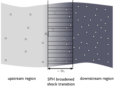
Figure 1: The shock structure in SPH simulations.

Our aim is to identify shock fronts in the MareNostrum Universe simulation and to derive the Mach number of the shocks. In order to estimate the radio emission produced by the shock, we will need the Mach number, downstream temperature and electron density. In SPH, energy is dissipated at shocks using an artificial viscosity. Most implementations of artificial viscosity follow the suggestions by Monaghan (1992) and Balsara (1995). In addition, viscosity-limiters are used to reduce spurious angular momentum transport in shear flows (Balsara, 1995; Steinmetz, 1996). In contrast to actually solving a Riemann problem, the SPH formalism does not identify any discontinuity. For our purpose it is sufficient to identify the shock fronts by post-processing snapshots of the simulation.

One possible approach is to extract the ratio of the upstream and downstream entropy. In SPH the dissipation rate is computed but the upstream and downstream entropy are never computed. The ratio of these two quantities would immediately give the strength of the shock. Pfrommer et al. (2006) determine the entropy gain in the shock by computing the product of the dissipation rate and the estimated crossing time of particles through the smoothed shock front. However, for particles in the SPH broadened shock front the analysis of local properties underestimates the strength of a shock. Pfrommer et al. (2006) cure this difficulty by using the maximum Mach number from within a certain time interval. As we wish to determine the Mach number from a single snapshot, we have developed the following scheme:

In the first step, for each SPH particle, we compute the entropy gradient, $\nabla S$. In a shock front this gradient gives the direction of the shock normal pointing into the downstream direction. We define an associated upstream position,

$${\bf x}_{{\rm u}i}={\bf x}_{i}+f_{h}\,h_{i}\,{\bf n}_{i}^{1},$$ (9)

where ${\bf x}_{i}$ is the position of the SPH particle $i$, $h_{i}$ the smoothing length of the particle $i$, and ${\bf n}_{i}^{1}$ denotes the shock normal, ${\bf n}_{i}^{1}=-\nabla S/|\nabla S|$. Moreover, we have introduced a factor $f_{h}$, chosen to be 1.3, which ensures that ${\bf x}_{{\rm u}i}$ is indeed in the upstream region and not in the transition between upstream and downstream properties. In a similar manner, we introduce an associated downstream position, ${\bf x}_{{\rm d}i}$, in the opposite direction.

Using the usual SPH scheme, we compute the density and internal energy at the upstream and downstream position. Moreover, we compute the velocity at these two positions and project it onto the shock normal. This results in the upstream and downstream velocity, $v_{{\rm u}i}+v_{\rm sh}={\bf v}({\bf x}_{{\rm u}i})\cdot{\bf n}_{i}^{1}$ and $v_{{\rm d}i}+v_{\rm sh}={\bf v}({\bf x}_{{\rm d}i})\cdot{\bf n}_{i}^{1}$, where $v_{\rm sh}$ is the velocity of the shock front in the rest-frame of the simulation. Since $v_{\rm sh}$ is not known, it is advantageous to assess only the differences $(v_{{\rm d}i}-v_{{\rm u}i})$. Beside a component parallel to the shock normal, the velocity field may also show perpendicular components. We compute these components in a similar manner to the upstream and downstream velocities, $v_{i}^{k\pm}={\bf v}({\bf x}_{i}\pm f_{h}h_{i}{\bf n}_{i}^{k})\cdot{\bf n}_{i}^{k}$, where the three vectors ${\bf n}^{1}$, ${\bf n}^{2}$, and ${\bf n}^{3}$ form an orthonormal base.

For those particles, that belong clearly to a shock front, we demand that the velocity has to be divergent in the direction of the shock normal, i. e. $(v_{\rm d}-v_{\rm u})>0$. Moreover, the velocity differences in the directions perpendicular to the shock normal have to be smaller than that parallel to the shock, $|v_{k}^{+}-v_{k}^{-}|<(v_{\rm d}-v_{\rm u})/2$. Therefore, the difference $(v_{\rm d}-v_{\rm u})$ gives roughly the velocity divergence.

There are two possibilities to compute the Mach number: First, we can evaluate the entropy ratio $q=S({\bf x}_{\rm d})/S({\bf x}_{\rm u})$. Secondly, we can use the ratio $(v_{\rm d}-v_{\rm u})/c_{\rm u}$. As discussed in Sec. 3.1, for both properties there exists a one-to-one mapping with the Mach number of the shock. We use a look-up table to obtain for both the entropy ratio and the velocity difference the corresponding Mach number. In order to have a conservative estimate for the Mach number we use the smaller of the two.

4 The radio emission model in a nutshell

At collisionless shock fronts a small fraction of particles may be accelerated to energies far beyond the thermal energy distribution. This has been directly observed in particle spectra of the Earth’s bow shock where the resulting momentum distribution depends strongly on the Mach number and the angle between shock normal and the direction of the upstream magnetic field. Also, the radio emission of solar bursts is generally attributed to shock-drift acceleration and subsequent excitation of plasma wave. Larger electron energies may be achieved by diffusive shock acceleration (DSA). The details of particle acceleration at collisionless shocks are complex and not fully understood yet. It is expected that DSA can operate in the ICM only with a starting energy above a few MeV, since at lower energies Coulomb losses are too efficient. Some electrons may attain this injection energy by shock-drift acceleration. It is beyond the scope of this paper to include a very detailed model for the processes at collisionless shock fronts. For simplicity, we assume that DSA operates already at thermal energies where Coulomb losses have to be compensated by acceleration mechanisms different from DSA. Following our model Hoeft & Brüggen (2007, HB07) we assume that supra-thermal electrons show a power-law spectrum, with a slope as predicted by DSA. We also suppose that a fixed fraction of the energy dissipated at the shock front is used to accelerate electrons. Finally, we assume that the supra-thermal electrons advect with the downstream plasma. In this section, we briefly introduce diffusive shock acceleration and review the model discussed in HB07. Moreover, we discuss our assumptions about the magnetic field. Finally, we present shock tube simulations that test our shock finder and allows us to calibrate the emission model.

4.1 Diffusive shock acceleration

In DSA, particles are accelerated by multiple shock crossings, in a first-order Fermi process. If the shock thickness is much smaller than the diffusion scale which, in turn, has to be much smaller than the curvature of the shock front, a one-dimensional diffusion-convection equation can be solved (Axford et al., 1978; Bell, 1978a, b; Blandford & Ostriker, 1978). The result is that the energy spectrum of suprathermal electrons is a power-law distribution, $n_{E}\propto E^{-s}$. The spectral index, $s$, of the accelerated particles is only related to the compression ratio at the shock front

$$s=\frac{r+2}{r-1}.$$ (10)

For strong, non-radiative shocks with Mach number $\gtrsim$10, the compression ratio is always close to 4, hence the slope $s$ is always close to 2. This can explain the spectrum of cosmic rays over a huge range of energies and may be considered a piece of evidence for DSA. For a review of diffuse shock acceleration see Drury (1983); Blandford & Eichler (1987); Jones & Ellison (1991); Malkov & O’C Drury (2001).

In supernova remnants, there is evidence that electrons and protons are accelerated by diffuse shock acceleration to energies of $\rm\sim 10^{15}\,eV$ (Berezhko et al., 2003; Vink & Laming, 2003).

4.2 Total emission induced by a shock front

In HB07 we have developed a model for the synchrotron emission from electrons that have been accelerated by DSA. Here, we summarise briefly the model and adapt it for the use in the framework of a SPH simulation. Our basic assumption is that a small fraction, $\xi_{\rm e}$, of the energy dissipated at the shock front is used to accelerate electrons to relativistic energies. The theory of diffusive shock acceleration predicts that the supra-thermal electron distribution obeys a power-law,

$$\frac{{\rm d}n_{\rm e}}{{\rm d}E}=C_{\rm spec}\,f_{\rm spec}(e,s)=C_{\rm spec}\,n_{\rm e}\frac{1}{m_{\rm e}c^{2}}\,e^{-s}\qquad{\rm for}\qquad e>e_{\rm min},$$ (11)

where $n_{\rm e}$ is the electron density and $C_{\rm spec}$ is a normalisation factor. The kinetic energy is measured in units of the electron rest mass, $e=E/m_{\rm e}c^{2}$. The energy $e_{\rm min}$ denotes the transition energy from the thermal Maxwell-Boltzmann distribution to the supra-thermal power-law distribution. In HB07 we have determined the normalisation factor,

$$C_{\rm spec}=\xi_{e}\frac{u_{\rm d}}{c^{2}}\frac{m_{\rm p}}{m_{\rm e}}\frac{(q-1)}{q}\frac{1}{F_{\rm spec}(e_{\rm min},s)},$$ (12)

where $F_{\rm spec}(e_{\rm min},s)$ is the integral of the power-law distribution without normalisation,

$$F_{\rm spec}(e_{\rm min},s)=\int\nolimits_{e_{\rm min}}^{\infty}\,{\rm d}e^{\prime}f(e^{\prime},s).$$ (13)

The transition energy, $e_{\rm min}$, has to be derived iteratively from the condition that supra-thermal electrons carry the fraction $\xi_{\rm e}$ of the kinetic energy.

For computing the radio emission we assume furthermore that the electrons are advected with the downstream plasma. This is justified since the electron gyro radii are small, orders of magnitude below one pc for any reasonable magnetic field strength and electron energy. Downstream electrons with $e\gtrsim 100$ cool mainly by synchrotron and inverse Compton losses (Sarazin, 1999). These electrons also contribute most to the detectable radio emission. For these two cool mechanisms the evolution of electron distribution function can be described analytically (Kardashev, 1962),

$$\frac{{\rm d}n_{\rm e}}{{\rm d}E}(t)=C_{\rm spec}\,n_{\rm e}\,\frac{1}{m_{\rm e}c^{2}}\>e^{-s}\left\{1-C_{\rm cool}\,e\,t\right\}^{s-2},$$ (14)

with

$$C_{\rm cool}=\frac{4\,\sigma_{\rm T}}{3\,m_{\rm e}\,c}\,\{u_{\rm CMB}+u_{B}\}.$$ (15)

Here $u_{\rm CMB}$ denotes the energy density of the cosmic microwave background, $u_{B}$ the energy density of the downstream magnetic field, and $\sigma_{\rm T}$ the Thomson cross section. We assume that in the zone relevant for radio emission the electron density and the magnetic field strength are constant. Evidently, the ICM varies in the region of the radio relics. We still ignore this effect since much larger uncertainties derive from our poor knowledge about the microphysics of collisionless shocks in the ICM.

The radio emissivity, $P(e,\nu_{\rm obs})$, depends on the energy of the electron energy, $e$, the observing frequency, $\nu_{\rm obs}$, and the magnetic field strength, $B$, (Rybicki & Lightman, 1986). Convolving the emissivity with the electron distribution, Eq. (14), and integrating over the downstream region results in the total emission behind the shock front,

$$\frac{{\rm d}P(\nu_{\rm obs})}{{\rm d}\nu}=m_{\rm e}c^{2}\,A\,\int\nolimits_{0}^{\infty}{\rm d}y\;\int_{E_{\rm min}}^{\infty}{\rm d}E\;\frac{{\rm d}n_{\rm e}}{{\rm d}E}(t(y))\>P(e,\nu_{\rm obs}),$$ (16)

where $y$ denotes the normal distance of a downstream location to the shock front, and $A$ is the surface area of the shock front. In HB07 we have evaluated the integral, Eq. (16). We found that the emission can be given by the shock surface area, the Mach number, the downstream temperature, the electron density, and the magnetic field strength,

$$\frac{{\rm d}P(\nu_{\rm obs})}{{\rm d}\nu} = 6.4\times 10^{34}\,{\rm erg\,s^{-1}\,Hz^{-1}}\;\;\frac{A}{{\rm Mpc^{2}}}\,\frac{n_{\rm e}}{\rm 10^{-4}cm^{-3}}\,$$

$$\quad\times\frac{\xi_{\rm e}}{0.05}\>\left(\frac{\nu_{\rm obs}}{\rm 1.4\,GHz}\right)^{-\frac{s}{2}}\left(\frac{T_{\rm d}}{\rm 7\,keV}\right)^{\frac{3}{2}}\>$$

$$\quad\times\frac{(B/{\rm\mu G})^{1+\frac{s}{2}}}{(B_{\rm CMB}/{\rm\mu G})^{2}+(B/{\rm\mu G})^{2}}\;\Psi({\cal M},T_{\rm d}).$$

The function $\Psi({\cal M},T_{\rm d})$ comprises all dependencies on the Mach number. Basically, $\Psi({\cal M},T_{\rm d})$ rises steeply for Mach numbers in the range 2 - 4 and is constant for large Mach numbers.

In HB07 we integrated Eq. (16) for a steady-state situation, where all time stages of the electron distribution function are present, from the newly accelerated distribution to a long time cooled spectrum. In a steady-state situation the overall synchrotron emission spectrum obeys a power-law. The slope of the spectrum is $s/2$, even though, locally, the slope may vary from the slope of newly accelerated electrons, $(s-1)/2$, to a very steep spectrum. This distribution of the spectral index agrees well with the observation for several radio relics (e. g. Orrú et al. (2007); Pizzo et al. (2008)).

As discussed in HB07 the integral, Eq. (16), can also be used to estimate the extent in $y$-direction, normal to the shock. We found that the extent depends mainly on the magnetic field. In the cluster centre the strength may be of the order of $1\,\mu{\rm G}$. In this case, 50 % of the radio emission comes from a region with a size of a few hundred kpc in $y$-direction, i. e. the size of the radio object is of the order of the size of the cluster centre. In contrast, in the cluster periphery the magnetic field strength may be of the order of $0.1\,\mu{\rm G}$. In this case, the extent of the emission region is about 100 kpc, which is significantly smaller than the scale of spatial variations in the cluster periphery. In the following, we assign the radio emission solely to the shock front and ignore the extent of the radio emission region in $y$-direction. This approach is perfectly suited for studying the radio emission in the cluster periphery, since there the downstream extend of the emission region is smaller than the numerical resolution. In the cluster centre our approach may lead to too compact radio objects.

The shock finder described in Sec. 3.2 allows us to locate shock discontinuities in a SPH simulation snapshot. The shock finder also provides estimates for the Mach number and for the shock normal. Using the normal vector, we can find a position which is sufficiently downstream to determine the downstream temperature, $T_{\rm d}$, and the electron density, $n_{\rm e}$, which are needed to compute the radio emission via Eq. (4.2). To compute the radio power, ${\rm d}P/{\rm d}\nu$, we also need the area, $A$, of the shock front. Since in SPH a shock front is comprised of particles, each particle represents an area of the shock. More precisely, the shock discontinuity is smoothed by the size of the SPH kernel, $h_{\rm SPH}$, see Fig. 1. The kernel may contain $N_{\rm SPH}$ particles, the corresponding volume is of the order of $h_{\rm SPH}^{3}$. Hence, one particle belonging to the shock front represents a shock area of

$$A=f_{A}\frac{h_{{\rm SPH}}^{2}}{N_{\rm SPH}},$$ (18)

where $f_{A}$ is a normalisation constant, which will be determined by the help of Sod shock tube simulations, see Sec. 4.4. Finally, we have to determine the downstream magnetic field strength. In the next paragraph, Sec. 4.3 we detail how we estimate $B_{\rm d}$.

4.3 Magnetic field model

The downstream magnetic field is crucial for the synchrotron emission. For a power-law electron energy distribution the emission is given by

$$P(\nu)\propto n_{\rm e}\,(B\sin\theta)^{1+\alpha}\,\nu^{-\alpha},$$ (19)

where $\theta$ is the pitch angle between the electron velocity and the magnetic field. The exponent $\alpha$ is related to the slope of the electron spectrum by $\alpha=(s-1)/2$. Unfortunately, in Eq. (19) the electron density and the field strength are degenerated. Therefore, evaluating only the synchrotron emission of diffuse radio objects in the ICM is not sufficient to derive the magnetic field strength. For some clusters it has been possible to measure the electron density by the hard X-ray excess in the cluster spectrum (see Rephaeli et al. (2008) for a review). As a result, the average cluster magnetic field strength has been estimated to be of the order of $0.1$ to $1\,{\rm\mu G}$ (Fusco-Femiano et al., 2001; Rephaeli & Gruber, 2003; Rephaeli et al., 2006). Alternatively, one assumes that the energy density of the ICM is minimal (Govoni & Feretti, 2004). This method also results in magnetic field strengths of the order of $0.1$ to $1\,{\rm\mu G}$. Contrarily, Faraday rotation measurement studies (see e. g. Govoni et al. (2006)) typically yield field strengths that are larger by about an order of magnitude.

The strength, structure and origin of magnetic fields in the ICM is still debated. Intergalactic magnetic fields may be a remainder of primordial processes, may be generated by a dynamo in first stars and subsequently expelled, may be generated by the Biermann battery effect during cosmic reionisation, may be caused by microinstabilities in the turbulent ICM, or may be generated at collisionless shock fronts. It is beyond the scope of this paper to include a detailed model for the generation and evolution of magnetic fields. Even the passive evolution of magnetic fields during cosmic structure formation is complex (Dolag et al., 2002; Brüggen et al., 2005). However, we assume here that the magnetic strength in the downstream region of the shock front, $B_{\rm d}$, on average simply obeys flux conservation to follow

$$\frac{B_{\rm d}}{B_{\rm ref}}=\left(\frac{n_{\rm d}}{10^{-4}\,{\rm cm^{-3}}}\right)^{2/3}.$$ (20)

4.4 Normalisation of the radio emission

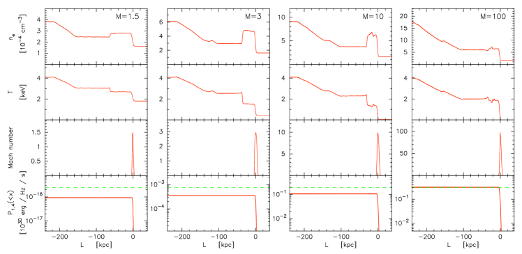
Figure 2: Simulations of the Sod shock tube problem with Mach numbers 1.5, 3, 10, 100. The upper panel shows the electron density assuming a fully ionised ICM, the second row the temperature, the third row the Mach number as determined by the Mach number estimator described in Sec. 3.2 and the lower panel the cumulative radio emission as described in Sec. 4.4 assuming an observation frequency of 1.4 GHz. Note that the irregularites in $n_{\rm e}$ and $T$ are caused by the small number of particles in the SPH kernel, namely $N_{\rm SPH}=40$. We choose this number in order to conform with the parameters used in the MareNostrum Universe simulation. For the shock finding we smoothed the fields to some extend by using $N_{\rm kernel}=80$ in the finder, see Tab. 1.

In our model it is necessary to determine the effective area of the shock front represented by one SPH particle, $A_{i}$, which may also depend on the actual Mach number. Therefore, we simulated the Sod shock tube problem and determine the Mach number by our method described in Sec. 3.2. As shown in Fig. 2, the original Mach number used to set up the initial conditions is well reproduced by the Mach number estimator. We have simulated shock tubes with Mach numbers from 1.5 to 100. This covers well the range of relevant Mach numbers for the radio emission of merger-induced and accretion shocks. In all cases, the theoretically expected Mach number is found in the centre of the transition region between the upstream and the downstream region. In the periphery the Mach number is underestimated, i. e. the particles in the shock region show a Mach number distribution, as shown in the third row of Fig. 2.

The theoretical value of the radio emission is easily computed via Eq. (4.2). The Mach number is known from setting up the initial conditions of a shock tube, and the properties of the downstream plasma are known from the analytic solution. In the simulation a large number of SPH particles contributes to the emission. To show the total emission we plot the cumulative radio emission, i. e. the emission, $P(x_{i})$, of all particles on the left-hand side of a given $x$-position is summed,

$$P(<x)=\sum\nolimits_{i}\,P(x_{i})\qquad{\rm with}\qquad x_{i}<x.$$ (21)

As noted above the Mach number estimator results in a distribution of Mach numbers for the particles in the SPH-broadened shock discontinuity. For small Mach numbers, ${\cal M}\lesssim 5$, the radio emission depends strongly on ${\cal M}$, while for large Mach numbers it does not. Hence, a constant area normalisation factor, $f_{A}$ (introduced in Sec. 4.2), would systematically underestimate the radio emission of shocks with ${\cal M}\lesssim 5$. One could correct for this effect by introducing a function $f_{A}({\cal M})$. However, we choose a somewhat simpler solution and increase the Mach number slightly when computing the radio emission for a particle,

$$\Psi({\cal M})\to\Psi({\cal M}\times 1.045).$$ (22)

As a result we are able to reproduce the expected radio emission of the different shock tubes with deviations smaller than a factor of three. Regarding the simplicity of our model (power-law electron spectrum, uniform energy fraction in supra-thermal electrons, flux conservation of magnetic field) this accuracy is sufficient.

Module	Parameter	Symbol	Value	See Sec. for details
MareNostrum Universe	mass dark matter part.	$m_{\rm DM}$	$8.3\times 10^{9}\>h^{-1}\,{{{\rm{M_{\odot}}}}}$	2
	mass gas particles	$m_{\rm gas}$	$1.5\times 10^{9}\>h^{-1}\,{{{\rm{M_{\odot}}}}}$
	force resolution	$r_{\rm soft}$	$15\>h^{-1}\,{\rm kpc}$ (comoving)
	SPH kernel	$N_{\rm SPH}$	40
Shock finder	shock extent factor	$f_{h}$	1.3	3.2
	part. number in kernel	$N_{\rm kernel}$	80	3.2
Mach number estimator	shock area fraction	$f_{A}$	6.5	4.2, 4.4
	Mach number correction	${\cal M}$	${\cal M}\times 1.045$	4.4
Radio emission	energy fract. in supra-thermal e-	$\xi_{\rm e}$	$5\times 10^{-3}$	4.2
	reference magn. field strength	$B_{\rm ref}$	$0.1{\>\mu{\rm G}}$	4.3

Table 1: Parameters used in the MareNostrum Universe simulation, for finding shock fronts, for estimating the Mach number, and for assigning the radio emission.

5 The radio emission in the simulation

We now wish to apply the tools prepared in the previous sections to estimate the radio emission of strong shocks which occur during cosmic structure formation. The most luminous diffuse radio emission is observed in massive clusters or their periphery. We therefore analyse massive clusters from a cosmological simulation. Our aim is to apply the radio emission model to the whole range of structure formation shocks, caused by mergers and gas accretion. In this paper we estimate only the radio emission which is originated by primary electrons.

We apply the Mach number estimator described in Sec. 3.2 and the radio emission model described in Sec. 4.2 to the MareNostrum Universe simulation described in Sec. 2. More precisely, we analyse the 300 most massive clusters with masses in the range 0.4 to $2.5\times 10^{15}h^{-1}{{{\rm{M_{\odot}}}}}$. We do not include less massive clusters since the resolution gets too poor. First we show the results of our Mach number estimator for a selection of clusters. Then, we present artificial observations and compare them to observed radio relics. Finally, we discuss how the radio emission correlates with X-ray temperature of the clusters.

5.1 The ICM in slices

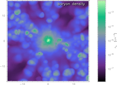
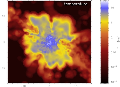
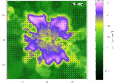
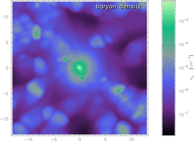
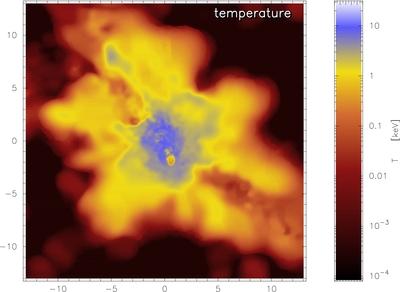
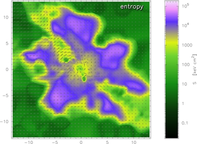
Figure 3: Density, temperature and entropy in a slice for two clusters. Each row represents one cluster. Density, temperature and entropy are computed for a slice through the cluster centre, by computing for each pixel the SPH average. Spatial scales are given in $h^{-1}\>{\rm Mpc}$. The virial radius on the two clusters is about $2\>h^{-1}\>{\rm Mpc}$. One can nicely see that gas gets heated at a few times the virial radius.

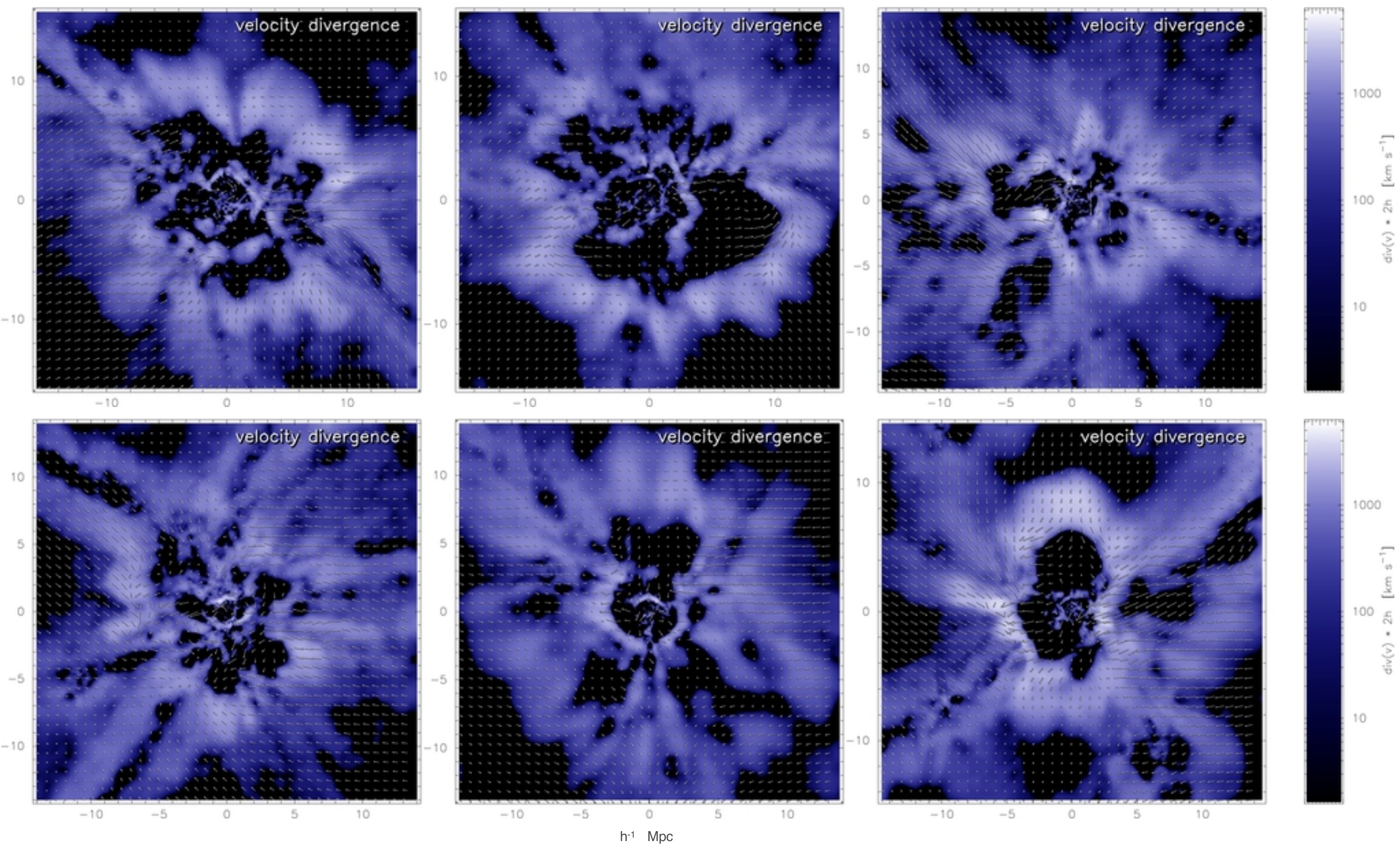
Figure 4: Velocity divergence in a slice through the cluster center for six different clusters of our sample. The velocity divergence refers here to the difference $(v_{\rm d}-v_{\rm u})$, see Sec. 3. One can clearly distinguish the outer ‘accretion’ shocks and the inner ‘merger’ shocks. Note that the width of the shocks is caused by the the numerical resolution, which is much poorer in the region of the accretion shocks than in inner region of the clusters.

It is instructive to consider the physical properties of the ICM in slices through the cluster, see Fig. 3. One can clearly see how the temperature rises sharply in the periphery of a cluster, far beyond the virial radius. At this location, about four times the viral radius, the ICM gets heated to cluster tempertaures, i. e. about $1\,{\rm keV}$, by accretion shocks. Within clusters, the temperature and entropy maps are complex, since rather cold intergalactic medium flows in filaments to the cluster centre and ongoing or past mergers lead to intricate gas flows. However, the velocity divergence reveals also the location of the inner merger shocks, see Fig. 4. Note that we compute the divergence according to the procedure described in Sec. 3, i. e. we determine first the shock normal and subsequently compute the difference $(v_{\rm d}-v_{\rm u})$. As also described in Sec. 3 the ratio of the velocity divergence and the upstream sound speed allows us to infer the Mach number of the shock. Additionally, the ratio of downstream and upstream entropy allows to determine the Mach number. We use the minimum of both for further analysis, i. e. for computing radio emission.

5.2 Visualising the shock fronts

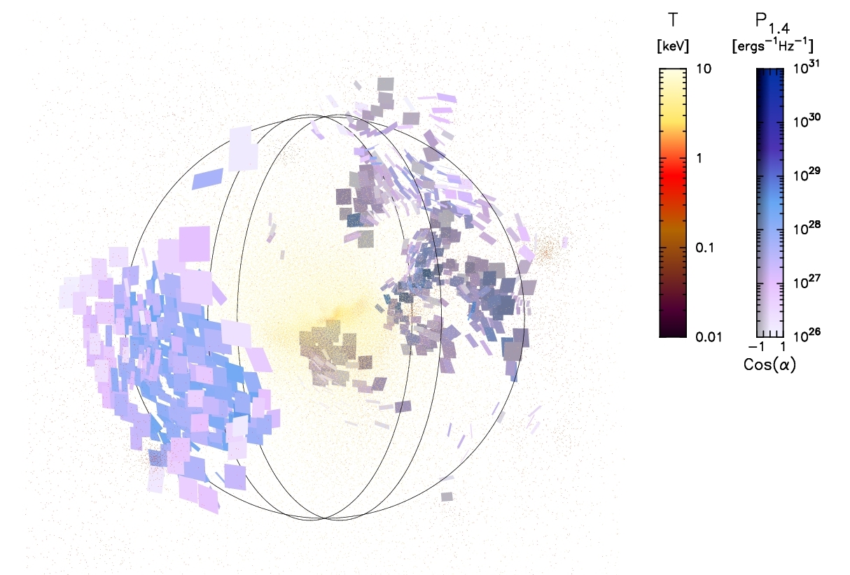
Figure 5: A textbook example of a double relic found in the MareNostrum Universe simulation.

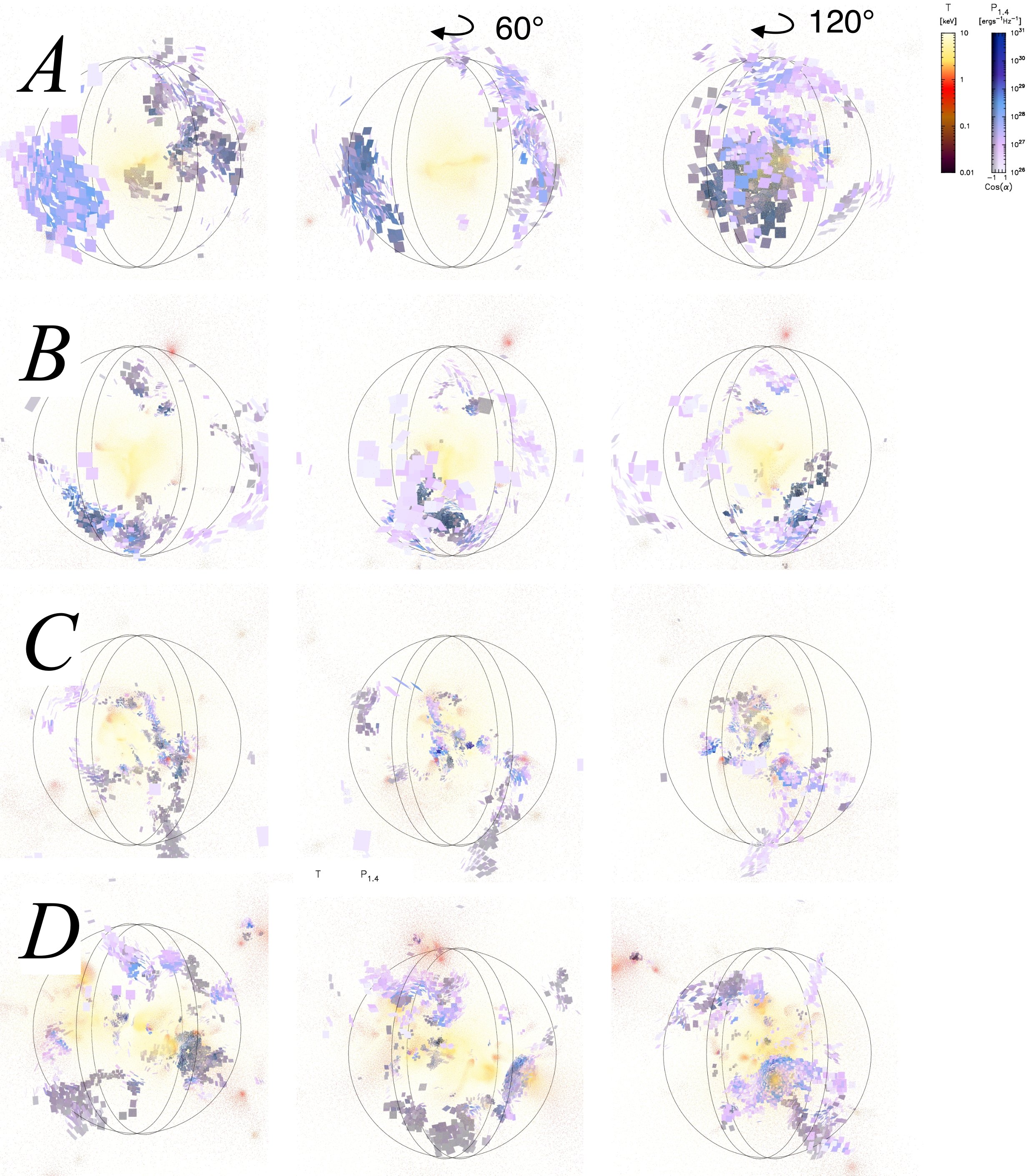
Figure 6: Radio emission and particle distribution for four typical galaxy clusters. The particles of the simulation are represented by dots with temperature colour-coded. Each SPH particles which belongs to a shock front a small square is drawn. The size of the square is proportional to the smoothing length of the particle. The colour gives the radio emission associated with the particle. Moreover we encode if a square is seen from upstream or the downstream direction. The latter are shaded grey. The circles indicate the viral radius of the galaxy cluster. See Tab. 2 for the properties of these exemplaric clusters. Each row represents one cluster, rotated by azimuthal angles of $60^{\circ}$ and $120^{\circ}$. See Fig. 7 for the projected radio emission.

Label	$L_{\rm bol}$	$T_{X}$	$M_{\rm vir}$	$t_{\rm merger}$	$P_{1.4}(<2R_{\rm vir})$	$\langle B_{\rm d}\rangle$	morphology has
	$[10^{44}\,\rm erg\,s^{-1}]$	$[\rm keV]$	$[10^{15}\,h^{-1}\,M_{\odot}]$	$[{\rm Gyr}]$	$[10^{31}\rm erg\,s^{-1}\,Hz^{-1}]$	$[{\rm\mu G}]$	similarities to
A	2.8	3.7	0.7	2.6	0.35	0.07	A3667, A3376
B	6.4	4.8	0.9	3.0	0.81	0.12	A115, A1664
C	50.4	12.2	1.5	3.1	8.56	0.79	A520
D	11.5	4.1	1.9	2.0	11.52	0.49
E	19.0	7.8	1.4	5.3	0.04	0.25
F	7.6	5.3	1.2	4.1	0.12	0.07
G	23.4	8.1	1.1	1.9	0.10	0.12
H	5.0	3.7	0.8	1.2	0.03	0.16

Table 2: Properteis of the selected clusters.

As seen in the slices through the clusters, the geometry of the strong shocks may be very complex. To visualise the shocks, we represent each of these particles by a small square to which the shock normal is perpendicular. Each of these square may be considered as a small part of the shock surface. The edge length of a square is proportional to the smoothing length of the corresponding SPH particle.

We color-code the squares by the radio emission computed for the corresponding SPH particle. Fig. 5 shows a text-book example of a double relic found in the MareNostrum Universe simulation. This cluster has developed two large shock fronts in the cluster periphery, similar to the radio objects found in A3667 (Röttgering et al., 1997) and A3376 (Bagchi et al., 2006). In addition to the emission of each SPH particle in the shock front, we color-code the orientation of the shock normal. We shade squares grey for which the normal points away from the observer, where the level of shading depends on the angle, $\alpha$, between shock normal and the direction to the observer. As a result, shock fronts which propagate towards the observer appear blueish while fronts which move away appear greyish.

To show the location of the cluster, we represent the SPH particles by dots with the temperature colour-coded. Infalling substructures can often be identified in temperature maps since they are usually much colder than the surrounding ICM. The clusters in the MareNostrum Universe simulation show radio objects with very different morphologies. In Fig. 6 four examples are displayed, each of which viewed from three different angles. As discussed above, cluster A contains a textbook example for a double relic. Cluster B shows only one relic which is composed of several smaller fragments. In cluster C, several strongly emitting sources in the centre of the cluster are found. Finally, cluster D shows the emission of an early state merger system. The temperature of this cluster is only about 4 keV (see Tab. 2), but still a strong radio relic has been developed.

The structure of the shock fronts can be seen best in an animation. We therefore encourage the reader to view the movies of the rotations of the four exemplary clusters available from our web site .

5.3 Radio maps

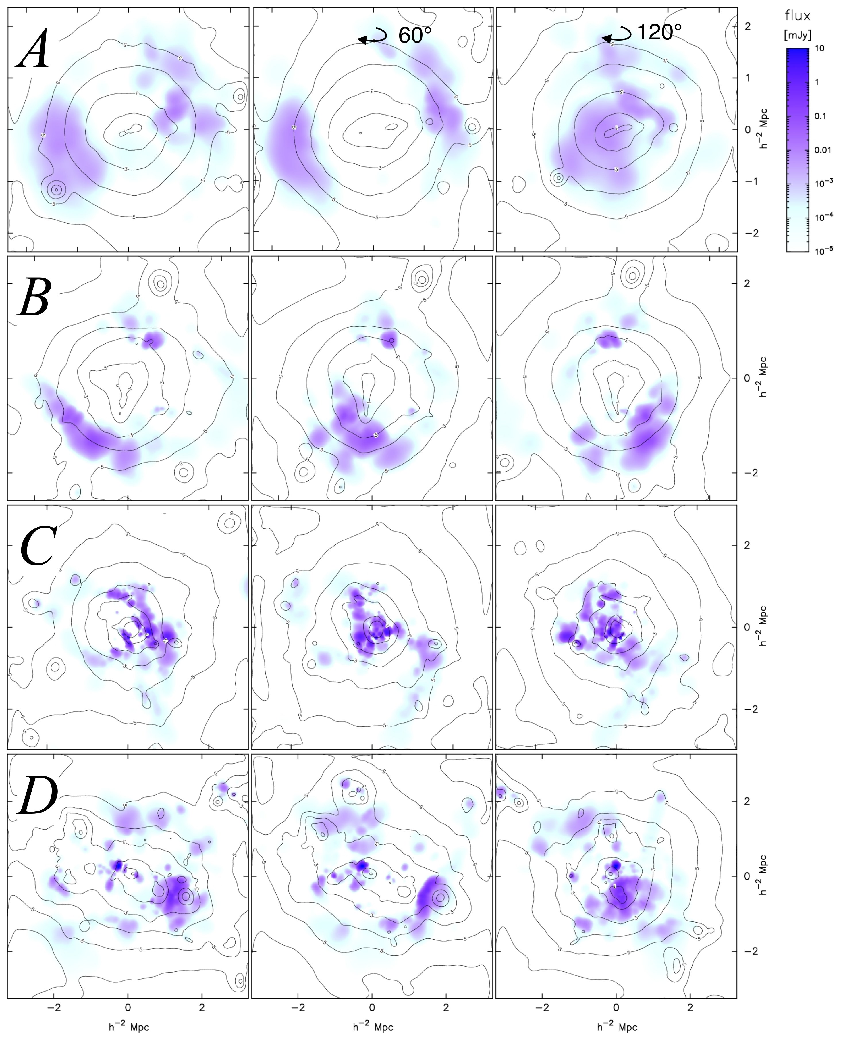
Figure 7: Mimic observations of the X-ray and the radio emission. We have projected the radio emission and bolometric X-ray emission of the clusters shown in Fig. 6. The radio flux at $1.4\,{\rm GHz}$ is computed for a hypothetical beam size of $10^{\prime\prime}\times 10^{\prime\prime}$. No redshift effects are taken into account.

Having assigned a radio luminosity to each SPH particle, we are able to compute artificial radio maps. To this end we project the emission of each particle along the line-of-sight and smooth it according to the SPH kernel size. We compute the radio emission for an observing frequency of 1.4 GHz and a hypothetical beam size of $10^{\prime\prime}\times 10^{\prime\prime}$. For comparison, we also compute contours of the bolometric X-ray flux. We follow Navarro et al. (1995) and assign each particle the luminosity

$$L_{X}=1.2\times 10^{24}\,{\rm erg\,s^{-1}}\>\frac{m_{\rm gas}}{\mu\,m_{\rm p}}\>\frac{n_{\rm e}}{\rm cm^{-3}}\left(\frac{T}{\rm keV}\right)^{1/2}.$$ (23)

Fig. 7 shows the artificial radio maps and the X-ray contours for the same clusters already presented in Fig. 6. The double relic structure of cluster A becomes even more prominent. The X-ray contours reveal for some viewing angles clearly the merger state of the clusters.

The examples in Fig. 7 and Fig. 6 are selected to illustrate the variety of diffuse radio objects obtained by our simple emission model. Example A shows the large-scale merger shocks that are also found in idealised merger simulations (e.g. Roettiger et al., 1999). In contrast, example C shows a large number of smaller shock fronts. Some of them are related to substructures moving through the ICM, while others are obviously unrelated to any substructure (this can be best seen in the animations mentioned above). The morphology of the radio emission resembles that found in A2255, where several rather small pieces of diffuse radio emission have been detected (Pizzo et al., 2008).

Another property of our model for diffuse radio emission is the fact that many of the massive clusters show no or only little radio emission. Therefore, we show four examples with almost radio-quiet clusters, see Fig. 8. Example E is the stereotype of a relaxed massive clusters. There is no large-scale shock present which can cause significant radio emission, only a very few small regions with a radio-loud shock are found. This is consistent with the time of the last major merger (the mass of the accreted substructure has to be at least 25 % of the main cluster), which has take place more than $5\,Gyr$ in the past. Examples D and F show a distorted X-ray morphology indicating recent merger activity. However, the resulting merger shocks are very faint in the radio. Finally, example G shows a merger in an early state with no radio emission. Hence, even with our simple radio emission model merger activity does not lead in all cases to strong radio emission. This is expected from modelling electron acceleration at the shock front, since a Mach number above 2.5 is needed for a significant amount of radio emission. Many of the merger shocks have lower Mach numbers.

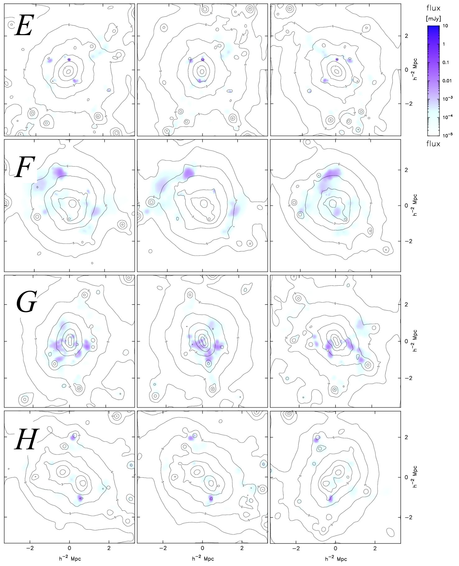
Figure 8: Mimic observations of the X-ray and the radio emission for four galaxy clusters with a low radio emission.

5.4 The luminosity function of radio objects

Figure 9: The cumulative number density of radio objects. The left axis give the number of objects found in the simulation box. The solid line indicates the number of radio objects as identified by splitting the objects in well separated groups (see Sec. 5.4). The long-dashed line gives the radio luminosity function for the clusters in MareNostrum Universe simulation. The radio power of a cluster includes all emission within the virial radius. For comparison we depict the radio halo luminosity function as computed by Enßlin & Röttgering (2002). We adopt their best fitting of the radio halo–X-ray correlation with $a_{\nu}=3.37$ and $b_{\nu}=1.69$.

As can be seen by the examples A to D, one can often divide the emitting structures into individual objects, such as the emission in front of a supersonically moving galaxy and that of a merger shock front travelling outwards in the ICM. In order to identify individual radio objects in our simulation, we select all particles whose radio emission lies above a very low threshold. For these particles we determine their nearest neighbours, and obtain as a result a spanning tree for radio-loud particles. We now cut all links that are larger than the minimum of the smoothing lengths of the two connected particles. As a result, the spanning tree separates into sub-trees, each of which can be considered an individual radio object. By this method we can for instance disentangle the radio emission of an infalling substructure from that of large merger shock. Finally, we compute the cumulative number of radio objects above a given luminosity, see Fig. 9, i. e. the luminosity function of diffuse radio objects. Most of the very luminous objects ($P_{1.4}\gtrsim 10^{32}\,{\rm erg\,s^{-1}\,Hz^{-1}}$) are rather small structures, similar to that seen in example C. The textbook merger shocks, as in example A, have only luminosities of the order of $10^{31}\,{\rm erg\,s^{-1}\,Hz^{-1}}$ and below. Therefore, the very luminous relics in A3667 seem to be very exceptional. Our textbook merger shocks are similar to the less luminous relics found in A3376 (Bagchi et al., 2006).

We choose the parameters of our model in a way that the resulting radio objects agree with observations in the respect that the most luminous ones have a radio power, $P_{1.4}$, of $\sim 10^{33}\,{\rm erg\,s^{-1}\,Hz^{-1}}$. Towards small luminosities the cumulative number of radio objects increases with a slope close to $-2/3$. For comparison we compute the radio luminosity within the virial radius of the clusters in the MareNostrum Universe simulation and find an even shallower curve. The rather shallow slope of the faint end of the radio luminosity function reflects that the radio luminosity depends strongly on the cluster mass or temperature. We will discuss this further in the next section.

For comparison we have shown in Fig. 9 the radio halo luminosity derived by Enßlin & Röttgering (2002). They concluded that the upcoming radio telescope Lofar could discover about 1000 radio halos by a survey in a years timescale. With the parameters used in our model we find a much larger abundance of radio objects. However, we may overestimate the efficiency of diffusive shock acceleration or the strength of magnetic fields. It is worth noticing that the slope of the radio luminosity function at the low-luminosity end is similar to that of Enßlin & Röttgering (2002), hence, one may expect the discovery of a large number of radio objects with Lofar. The radio luminosity function of clusters is significantly flatter, indicating that one cluster may contain several radio objects with moderate luminosity. As a result we expect that the number of cluster for which Lofar will find new radio features is significantly lower than 1000. However, for a more quantitative analysis model parameters have to be normalised and the redshift evolution has to be included properly. This will be discussed in a forthcoming paper.

5.5 Radio versus X-ray

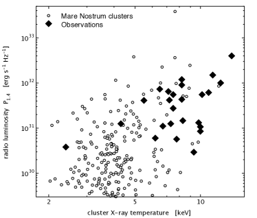
Figure 10: Bolometric X-ray temperature versus radio luminosity. For comparison observational data are shown. The data include radio relics and halos (Govoni et al. (2001), Govoni & Feretti (2004), Feretti et al. (1997), Liang et al. (2000), Giovannini et al. (1999) ).

We also estimate the radio–X-ray correlation of the galaxy clusters in our simulation by computing the bolometric X-ray luminosity and the emission-weighted temperature. Fig. 10 shows that only a fraction of the clusters is very luminous in radio, meaning that they show a radio luminosity above $10^{31}\,{\rm erg\,s^{-1}\,Hz^{-1}}$. This is also true for a significant number of the massive, i. e. hot, clusters. However, the maximum radio luminosity scales strongly with the cluster temperature. This is indeed expected for radio relics the most massive clusters (see e.g. Feretti et al., 2004). We plot for comparison the radio luminosity of several radio relics and halos. The MareNostrum Universe simulation clusters show a trend similar to the observed ones, however, the radio luminosity of our clusters is in average higher than that of the observed clusters. This difference may be caused by our assumptions for the parameters in the radio emission model, i. e. the shock acceleration is too efficient in our model, or the magnetic fields are too strong. Alternatively, the X-ray temperature of the simulated clusters might be too low. In a forthcoming work we will use the comparison to observed radio halos and relics to constrain our model parameters. Here we wish to point out that our simple emission model taking only primary electrons into account nicely restores in combination with a cosmological simulation the fact that only a small fraction of clusters show luminous diffuse radio structures and in addition the trend in the radio luminosity–X-ray relation.

5.6 Radio emission of accretion shocks

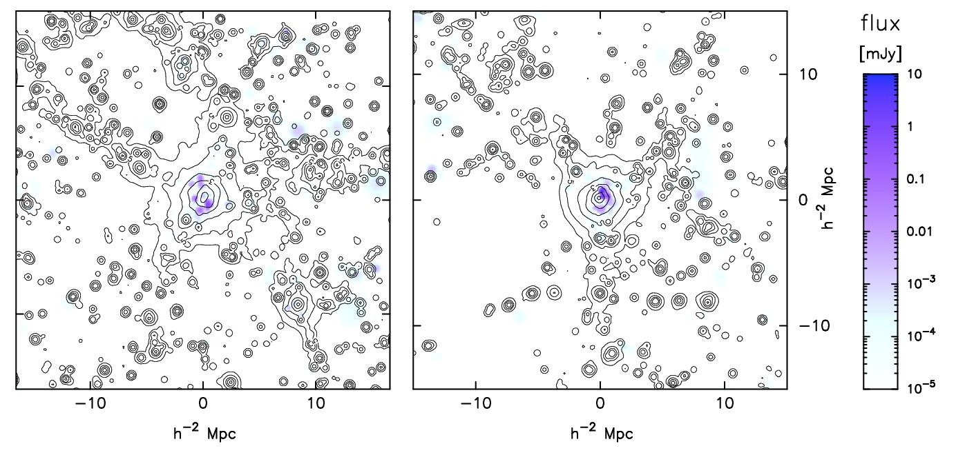
Figure 11: Mimic observations of the X-ray and the radio emission of the periphery of the two most massive clusters in the MareNostrum Universe simulation.

Our method also allows to study the radio emission of accretion shocks. Here we show artificial radio maps for two of the most massive clusters in the simulation using a larger field-of-view, see Fig. 11. We find only very little emission in the region of the accretion shocks, which are roughly located at four times the virial radius, i. e. $\sim 10\,h^{-1}\,{\rm Mpc}$ for the two most massive clusters. The reason is that the temperature, density and magnetic field are simultaneously low in the cluster periphery. As a result the two clusters shown in Fig. 11 have a radio emission even below $10^{-4}\,{\rm mJy}$ (for a $10^{\prime\prime}\times 10^{\prime\prime}$ beam). Hence, it may be difficult even with the sensitivity of upcoming radio telescopes to detect the accretion shock by their radio emission.

5.7 Magnetic field strength in radio relics

Magnetic fields in the region of radio relics are difficult to determine observationally since the field strength and the number density of relativistic electrons are degenerated in the expression for the radio luminosity. Estimates for ICM magnetic fields range from 0.1 to $10\,{\rm\mu G}$. We compute the radio luminosity-averaged magnetic field within two times the virial radius for the sample of clusters presented here in detail, see Tab. 2. More precisely, we compute

$$\langle B_{\rm d}\rangle=\frac{1}{P_{1.4}(<2r_{\rm vir})}\sum\nolimits_{r_{i}<2r_{\rm vir}}\,P_{1.4}({\bf r}_{i})B_{\rm d}({\bf r}_{i}).$$

We find that that for the clusters presented here the average magnetic field strength is in the range of 0.07 to $0.8\,{\rm\mu G}$. Despite general over-luminosity of of the radio objects generated in our simulation the magnetic fields in the downstream region has been modelled with moderate field strength only. This implies that the abundance of radio relics in general can be explained with rather weak magnetic fields in the periphery of galaxy clusters.

6 Discussion and Summary

We have presented a novel method for estimating the radio emission of strong shocks that occur during the process of structure formation in the universe. Our approach is based on an estimate for the shock surface area and we compute the radio emission per surface element using the Mach number of the shock and the downstream plasma properties. The advantage of our method is that we can accurately determine the emission of the downstream regime without using an approximate, discretised electron spectrum. The disadvantage is clearly that we do not include any evolution of the shock front and the downstream medium. However, our main goal here is to compute the radio emission from all shock fronts generated during cosmic structure formation. Our main assumption is that radio emission is caused by primary electrons accelerated at the shock front. To obtain a model suitable for the application in the framework of a cosmological simulation we have to neglect the complexity of collisonless shocks, details of the electron acceleration mechanisms, the amplification of magnetic fields by upstream cosmic rays, and so forth. The model reflects rather an expectation for the average radio emission entailed by structure formation shocks.

Our results show that in a cosmological simulation one indeed finds textbook examples for large-scale, ring-like radio relics as observed in A3667 and A3376. Our example A shows two large half-shell shaped shock fronts and no radio emission in the centre of the merging cluster. However, cluster A is not very massive, hence the radio luminosity of the two half-shells is low compared to A3667. Another nice example is cluster B which shows a radio relic only one side of the cluster, similar to A115. Beside those spectacular relics in the periphery of galaxy clusters, we find that a lot of clusters show complex, radio-loud shock structures close to the cluster centre. This suggests that part of the central diffuse radio emission in galaxy clusters, i. e.the radio halo phenomena, can be attributed to synchrotron emission of primary electrons.

We have modelled the radio emission with conservative assumptions for the efficiency of shock acceleration, namely $\xi_{e}=0.005$, and for the strength of magnetic fields in the downstream region, namely of the order of 0.07 to $0.8\,{\rm\mu G}$. Still, we find that the radio luminosity in the cluster region is on average significantly above observed values, see Fig. 9. Even lower values for the acceleration efficiency or the magnetic field strength would suffice to explain the abundance of diffuse radio objects on the sky. In conclusion, our findings support the scenario in which radio relics are generated by primary electrons.

In summary, we have analysed one of the largest hydrodynamical simulations of cosmic structure formation with respect to shock fronts in clusters of galaxies. We have developed a method to identify the shock fronts, to estimate their Mach numbers and their orientation. We have applied the method described in Hoeft & Brüggen (2007) to determine the radio emission as a function of the shock surface area and the downstream plasma properties. Our analysis led to the following results:

• By evaluating the entropy and the velocity field we are able to identify strong shocks in the simulation and to determine their properties.

• Using conservative values for the efficiency of strong shocks to accelerate electrons and for strengths of magnetic fields, we are able to reproduce the number density and the luminosity of large-scale radio relics. Only a very few of the most massive clusters show such luminous, extended sources.

• Our model reproduces various spectacular sources of diffuse radio emission at the periphery of galaxy clusters. Other clusters show emission with complex morphology close to the cluster centre. These sources may be classified as part of a central radio halo, following the observational distinction between relics and halos.

• Our results reproduce the strong correlation between radio luminosity and cluster temperature. The highest radio luminosities occur in dense and hot environments such as massive clusters. In addition we find that a large number of galaxy clusters show only little diffuse radio emission.

• We find that the abundance of radio relics can be explained with efficiency of diffusive shock acceleration for electrons lower than $\xi_{e}=0.005$ and a strength of magnetic fields in the relic region lower than 0.07 to $0.8\,{\rm\mu G}$.

• All of the luminous radio relics belong to internal shock fronts. The accretion shocks are located at larger distances from the cluster centre. Since density and temperature are low at this location, their luminosity is too small to reach a similar flux as internal shock fronts.

Acknowledgment

MH acknowledges DLR funding under the grant 50 OX 0201. MB acknowledges the support by the DFG grant BR 2026/3. The MareNostrum Universe simulations have been done at the Barcelona Supercomputing Center (Spain) and analysed at NIC Jülich (Germany). GY thanks MEC (Spain) for financial support under project numbers FPA2006-01105 and AYA2006-15492-C03. Our collaboration has been supported by the European Science Foundation (ESF) for the activity entitled ‘Computational Astrophysics and Cosmology’ (AstroSim).

References

- Axford et al. (1978) Axford, W. I., Leer, E., & Skadron, G. 1978, in International Cosmic Ray Conference, 132–137
- Bacchi et al. (2003) Bacchi, M., Feretti, L., Giovannini, G., & Govoni, F. 2003, A&A, 400, 465
- Bagchi et al. (2006) Bagchi, J., Durret, F., Neto, G. B. L., & Paul, S. 2006, Science, 314, 791
- Balsara (1995) Balsara, D. S. 1995, Journal of Computational Physics, 121, 357
- Bell (1978a) Bell, A. R. 1978a, MNRAS, 182, 147
- Bell (1978b) —. 1978b, MNRAS, 182, 443
- Berezhko et al. (2003) Berezhko, E. G., Ksenofontov, L. T., & Völk, H. J. 2003, A&A, 412, L11
- Blandford & Eichler (1987) Blandford, R., & Eichler, D. 1987, PhysRep, 154, 1
- Blandford & Ostriker (1978) Blandford, R. D., & Ostriker, J. P. 1978, ApJL, 221, L29
- Brüggen et al. (2005) Brüggen, M., Ruszkowski, M., Simionescu, A., Hoeft, M., & Dalla Vecchia, C. 2005, ApJL, 631, L21
- Burgess (2007) Burgess, D. 2007, in Lecture Notes in Physics, Berlin Springer Verlag, Vol. 725, Lecture Notes in Physics, Berlin Springer Verlag, ed. K.-L. Klein & A. L. MacKinnon, 161–+
- Cen & Ostriker (1999) Cen, R., & Ostriker, J. P. 1999, ApJ, 514, 1
- Deiss et al. (1997) Deiss, B. M., Reich, W., Lesch, H., & Wielebinski, R. 1997, A&A, 321, 55
- Dolag et al. (2002) Dolag, K., Bartelmann, M., & Lesch, H. 2002, A&A, 387, 383
- Drury (1983) Drury, L. O. 1983, Reports of Progress in Physics, 46, 973
- Enßlin et al. (1998) Enßlin, T. A., Biermann, P. L., Klein, U., & Kohle, S. 1998, A&A, 332, 395
- Enßlin & Brüggen (2002) Enßlin, T. A., & Brüggen, M. 2002, MNRAS, 331, 1011
- Enßlin & Gopal-Krishna (2001) Enßlin, T. A., & Gopal-Krishna. 2001, A&A, 366, 26
- Enßlin et al. (2007) Enßlin, T. A., Pfrommer, C., Springel, V., & Jubelgas, M. 2007, A&A, 473, 41
- Enßlin & Röttgering (2002) Enßlin, T. A., & Röttgering, H. 2002, A&A, 396, 83
- Feretti (2005) Feretti, L. 2005, Advances in Space Research, 36, 729
- Feretti (2006) —. 2006, ArXiv Astrophysics e-prints
- Feretti et al. (2004) Feretti, L., Burigana, C., & Enßlin, T. A. 2004, New Astronomy Review, 48, 1137
- Feretti et al. (1997) Feretti, L., Giovannini, G., & Bohringer, H. 1997, New Astronomy, 2, 501
- Fusco-Femiano et al. (2001) Fusco-Femiano, R., Dal Fiume, D., Orlandini, M., Brunetti, G., Feretti, L., & Giovannini, G. 2001, ApJL, 552, L97
- Giovannini & Feretti (2004) Giovannini, G., & Feretti, L. 2004, Journal of Korean Astronomical Society, 37, 323
- Giovannini et al. (2006) Giovannini, G., Feretti, L., Govoni, F., Murgia, M., & Pizzo, R. 2006, Astronomische Nachrichten, 327, 563
- Giovannini et al. (1999) Giovannini, G., Tordi, M., & Feretti, L. 1999, New Astronomy, 4, 141
- Gottlöber & Yepes (2007) Gottlöber, S., & Yepes, G. 2007, ApJ, 664, 117
- Govoni & Feretti (2004) Govoni, F., & Feretti, L. 2004, International Journal of Modern Physics D, 13, 1549
- Govoni et al. (2001) Govoni, F., Feretti, L., Giovannini, G., Böhringer, H., Reiprich, T. H., & Murgia, M. 2001, A&A, 376, 803
- Govoni et al. (2006) Govoni, F., Murgia, M., Feretti, L., Giovannini, G., Dolag, K., & Taylor, G. B. 2006, A&A, 460, 425
- Hoeft & Brüggen (2007) Hoeft, M., & Brüggen, M. 2007, MNRAS, 375, 77
- Hoeft et al. (2004) Hoeft, M., Brüggen, M., & Yepes, G. 2004, MNRAS, 347, 389
- Jones & Ellison (1991) Jones, F. C., & Ellison, D. C. 1991, Space Science Reviews, 58, 259
- Jubelgas et al. (2008) Jubelgas, M., Springel, V., Enßlin, T., & Pfrommer, C. 2008, A&A, 481, 33
- Kang & Jones (2007) Kang, H., & Jones, T. W. 2007, Astroparticle Physics, 28, 232
- Kardashev (1962) Kardashev, N. S. 1962, Soviet Astronomy, 6, 317
- Kempner & Sarazin (2001) Kempner, J. C., & Sarazin, C. L. 2001, ApJ, 548, 639
- Kim et al. (1989) Kim, K.-T., Kronberg, P. P., Giovannini, G., & Venturi, T. 1989, Nature, 341, 720
- Klypin et al. (1999) Klypin, A., Gottlöber, S., Kravtsov, A. V., & Khokhlov, A. M. 1999, ApJ, 516, 530
- Landau & Lifshitz (1959) Landau, L. D., & Lifshitz, E. M. 1959, Fluid mechanics (Course of theoretical physics, Oxford: Pergamon Press, 1959)
- Liang et al. (2000) Liang, H., Hunstead, R. W., Birkinshaw, M., & Andreani, P. 2000, ApJ, 544, 686
- Malkov & O’C Drury (2001) Malkov, M. A., & O’C Drury, L. 2001, Reports of Progress in Physics, 64, 429
- Miniati (2001) Miniati, F. 2001, Computer Physics Communications, 141, 17
- Miniati (2004) —. 2004, Journal of Korean Astronomical Society, 37, 465
- Miniati (2007) —. 2007, Journal of Computational Physics, 227, 776
- Miniati et al. (2001) Miniati, F., Jones, T. W., Kang, H., & Ryu, D. 2001, ApJ, 562, 233
- Miniati et al. (2000) Miniati, F., Ryu, D., Kang, H., Jones, T. W., Cen, R., & Ostriker, J. P. 2000, ApJ, 542, 608
- Monaghan (1992) Monaghan, J. J. 1992, ARA&A, 30, 543
- Navarro et al. (1995) Navarro, J. F., Frenk, C. S., & White, S. D. M. 1995, MNRAS, 275, 720
- Orrú et al. (2007) Orrú, E., Murgia, M., Feretti, L., Govoni, F., Brunetti, G., Giovannini, G., Girardi, M., & Setti, G. 2007, A&A, 467, 943
- Pfrommer et al. (2008) Pfrommer, C., Enßlin, T. A., & Springel, V. 2008, MNRAS, 385, 1211
- Pfrommer et al. (2006) Pfrommer, C., Springel, V., Enßlin, T. A., & Jubelgas, M. 2006, MNRAS, 367, 113
- Pizzo et al. (2008) Pizzo, R. F., de Bruyn, A. G., Feretti, L., & Govoni, F. 2008, A&A, 481, L91
- Rephaeli & Gruber (2003) Rephaeli, Y., & Gruber, D. 2003, ApJ, 595, 137
- Rephaeli et al. (2006) Rephaeli, Y., Gruber, D., & Arieli, Y. 2006, ApJ, 649, 673
- Rephaeli et al. (2008) Rephaeli, Y., Nevalainen, J., Ohashi, T., & Bykov, A. M. 2008, Space Science Reviews, 16
- Roettiger et al. (1999) Roettiger, K., Burns, J. O., & Stone, J. M. 1999, ApJ, 518, 603
- Rottgering et al. (2006) Rottgering, H. J. A., Braun, R., Barthel, P. D., van Haarlem, M. P., Miley, G. K., Morganti, R., Snellen, I., Falcke, H., de Bruyn, A. G., Stappers, R. B., Boland, W. H. W. M., Butcher, H. R., de Geus, E. J., Koopmans, L., Fender, R., Kuijpers, J., Schilizzi, R. T., Vogt, C., Wijers, R. A. M. J., Wise, M., Brouw, W. N., Hamaker, J. P., Noordam, J. E., Oosterloo, T., Bahren, L., Brentjens, M. A., Wijnholds, S. J., Bregman, J. D., van Cappellen, W. A., Gunst, A. W., Kant, G. W., Reitsma, J., van der Schaaf, K., & de Vos, C. M. 2006, ArXiv Astrophysics e-prints
- Röttgering et al. (1997) Röttgering, H. J. A., Wieringa, M. H., Hunstead, R. W., & Ekers, R. D. 1997, MNRAS, 290, 577
- Rybicki & Lightman (1986) Rybicki, G. B., & Lightman, A. P. 1986, Radiative Processes in Astrophysics (Radiative Processes in Astrophysics, by George B. Rybicki, Alan P. Lightman, pp. 400. ISBN 0-471-82759-2. Wiley-VCH , June 1986.)
- Ryu & Kang (2008) Ryu, D., & Kang, H. 2008, ArXiv e-prints, 806
- Ryu et al. (2003) Ryu, D., Kang, H., Hallman, E., & Jones, T. W. 2003, ApJ, 593, 599
- Sarazin (1999) Sarazin, C. L. 1999, ApJ, 520, 529
- Skillman et al. (2008) Skillman, S. W., O’Shea, B. W., Hallman, E. J., Burns, J. O., & Norman, M. L. 2008, ArXiv e-prints, 806
- Slee et al. (2001) Slee, O. B., Roy, A. L., Murgia, M., Andernach, H., & Ehle, M. 2001, AJ, 122, 1172
- Springel (2005) Springel, V. 2005, MNRAS, 364, 1105
- Steinmetz (1996) Steinmetz, M. 1996, MNRAS, 278, 1005
- Vink & Laming (2003) Vink, J., & Laming, J. M. 2003, ApJ, 584, 758
- Yepes et al. (2007) Yepes, G., Sevilla, R., Gottlöber, S., & Silk, J. 2007, ApJL, 666, L61