The optimal filters for the construction of the ensemble pulsar time

Abstract

The algorithm of the ensemble pulsar time based on the optimal Wiener filtration method has been constructed. This algorithm allows the separation of the contributions to the post-fit pulsar timing residuals of the atomic clock and pulsar itself. Filters were designed with the use of the cross- and autocovariance functions of the timing residuals. The method has been applied to the timing data of millisecond pulsars PSR B1855+09 and PSR B1937+21 and allowed the filtering out of the atomic scale component from the pulsar data. Direct comparison of the terrestrial time TT(BIPM06) and the ensemble pulsar time PT_ens revealed that fractional instability of TT(BIPM06)–PT_ens is equal to $\sigma_{z}=(0.8\pm 1.9)\cdot 10^{-15}$. Based on the $\sigma_{z}$ statistics of TT(BIPM06)–PT_ens a new limit of the energy density of the gravitational wave background was calculated to be equal to $\Omega_{g}h^{2}\sim 3\cdot 10^{-9}$.

1 Introduction

The discovery of pulsars in 1967 [Hewish et al. 1968] showed clearly that their rotational stability allowed them to be used as astronomical clocks. This became even more obvious after discovery of the millisecond pulsar PSR B1937+21 in 1982 [Backer et al. 1982]. Now a typical accuracy of measuring the time of arrivals (TOA) of millisecond pulsar pulses comprises a few microseconds and even hundreds of nanoseconds for some pulsars. For the observation interval in the order $10^{8}$ seconds this accuracy produces a fractional instability of $10^{-15}$, which is comparable to the fractional instability of atomic clocks. Such a high stability cannot but used for time metrology and time keeping.

There are several papers considering applicability of stability of pulsar rotation to time scales. The paper [Guinot 1988] presents principles of the establishment of TT (Terrestrial Time) with the main conclusion that one cannot rely on the single atomic standard before authorised confirmation and, for pulsar timing, one should use the most accurate realisations of terrestrial time TT(BIPMXX) (Bureau International des Poids et Mesures). The paper of Ilyasov et. al. [1989] describes the principles of a pulsar time scale, definition of ”pulsar second” is presented. Guinot & Petit (1991) show that, because of the unknown pulsar period and period derivative, rotation of millisecond pulsars is only useful for investigations of time scale stability a posteriori and with long data spans. The papers [Ilyasov et al. 1996], [Kopeikin 1997], [Rodin, Kopeikin & Ilyasov 1997], [Ilyasov, Kopeikin & Rodin 1998] suggest a binary pulsar time (BPT) scale based on the motion of a pulsar in a binary system with theoretical expressions for variations in rotational and binary parameters depending on the observational interval. The main conclusion is that BPT at short intervals is less stable than the conventional pulsar time scale (PT), but at a longer period of observation ($10^{2}\div 10^{3}$ years) the fractional instability of BPT may be as accurate as $10^{-14}$. The paper of Petit & Tavella [1996] presents an algorithm of a group pulsar time scale and some ideas about the stability of BPT. The paper of Foster & Backer [1990] presents a polynomial approach for describing clock & ephemeris errors and the influence of gravitational waves passing through the Solar system.

In this paper the author presents a method of obtaining corrections of the atomic time scale relative to PT from pulsar timing observations. The basic idea of the method was published earlier in the paper [Rodin 2006].

In Sect. 2, the main formulae of pulsar timing are described. Sect. 3 contains theoretical algorithm of Wiener filtering. Sect. 5 presents the results of numerical simulation, i.e. recovery of harmonic signal from noisy data by Wiener optimal filter and weighted average algorithm. The latter one is used similarly to the paper of Petit & Tavella [1996]. Sect. 6 describes an application of the algorithm to real timing data of pulsars PSR B1855+09 and PSR B1937+21 [Kaspi, Taylor & Ryba 1994].

2 Pulsar timing

The algorithm of the pulsar timing is widely described in the literature [Backer & Hellings, 1986], [Doroshenko & Kopeikin 1990], [Edwards, Hobbs & Manchester 2006]. Two basic equations are presented below. Expression for the pulsar rotational phase $\phi(t)$ can be written in the following form:

$$\phi(t)=\phi_{0}+\nu t+\frac{1}{2}\dot{\nu}{t}^{2}+\varepsilon(t),$$ (1)

where $t$ is the barycentric time, $\phi_{0}$ is the initial phase at epoch $t=0$, $\nu$ and $\dot{\nu}$ are the pulsar spin frequency and its derivative respectively at epoch $t=0$, and $\varepsilon(t)$ is the phase variations (timing noise). Based on the eq. (1) pulsar rotational parameters $\nu$ and $\dot{\nu}$ can be determined.

The relationship between the time of arrival of the same pulse to the Solar system barycentre $t$ and to observer site $\hat{t}$ can be described by the following equation [Murray, 1986]

$$c(\hat{t}-t)=-({\bf k}\cdot{\bf b})+\frac{1}{2R}[{\bf k}\times{\bf b}]^{2}+\Delta t_{\rm rel}+\Delta t_{DM},$$ (2)

where ${\bf k}$ is the barycentric unit vector directed to the pulsar, ${\bf b}$ is radius-vector of the radio telescope, $R$ is a distance to the pulsar, $\Delta t_{\rm rel}$ is the gravitational delay caused by the space-time curvature, $\Delta t_{DM}$ is the plasma delay. The pulsar coordinates, proper motion and distance are obtained from the eq. (2) by fitting procedure that includes adjustment of above-mentioned parameters for minimising the weighted sum of squared differences between $\phi(t)$ and the nearest integer.

3 Filtering technique

Let us consider $n$ uniform measurements of a random value (post-fit timing residuals) ${\bf r}=(r_{1},r_{2},\ldots,r_{n})$. ${\bf r}$ is a sum of two uncorrelated values ${\bf r}={\bf s}+\varepsilon$, where ${\bf s}$ is a random signal to be estimated and associated with clock contribution, $\varepsilon$ is random error associated with fluctuations of pulsar rotation. Both values ${\bf s}$ and $\varepsilon$ should be related to the ideal time scale since pulsars in the sky ”do not know” about time scales used for their timing. The problem of Wiener filtration is concluded in estimation of the signal ${\bf s}$ if measurements ${\bf r}$ and covariances (3) are given [Wiener 1949, Gubanov 1997]. For ${\bf r}$, ${\bf s}$ and $\varepsilon$ their covariance functions can be written as follows

$$\begin{array}[]{l}{\rm cov}(r,r)=\left<r_{i},r_{j}\right>=\left<s_{i},s_{j}\right>+\left<\varepsilon_{i},\varepsilon_{j}\right>,\\ {\rm cov}(s,s)=\left<s_{i},s_{j}\right>,\\ {\rm cov}(s,r)=\left<s_{i},r_{j}\right>=\left<r_{i},s_{j}\right>=\left<s_{i},s_{j}\right>,\\ {\rm cov}(\varepsilon,\varepsilon)=\left<\varepsilon_{i},\varepsilon_{j}\right>.\end{array}(i,j=1,2,\ldots,n)$$ (3)

$\left<\right>$ denominates the ensemble average.

The optimal Wiener estimation of the signal ${\bf s}$ and a posteriori estimation of its covariance function ${\bf D}_{ss}$ are expressed by formulae [Wiener 1949, Gubanov 1997]

$${\bf\hat{s}}={\bf Q}_{sr}{\bf Q}_{rr}^{-1}{\bf r}={\bf Q}_{ss}{\bf Q}_{rr}^{-1}{\bf r}={\bf Q}_{ss}({\bf Q}_{ss}+{\bf Q}_{\varepsilon\varepsilon})^{-1}{\bf r}$$ (4)

and

$${\bf D}_{ss}={\bf Q}_{ss}-{\bf Q}_{sr}{\bf Q}_{rr}^{-1}{\bf Q}_{rs},$$ (5)

where covariance matrices ${\bf Q}_{rr}$, ${\bf Q}_{sr}$, ${\bf Q}_{rs}$, ${\bf Q}_{ss}$ are constructed as Toeplitz matrices from the corresponding covariances. In this paper we assume that processes ${\bf s}$ and $\varepsilon$ are stationary in a weak sense (stationary are the first and second moments). Since quadratic fit eliminates the non-stationary part of a random process [Kopeikin 1999], their covariance functions depend on the difference of the time moments $t_{i}-t_{j}$.

Since it is impossible to perform pulsar timing observations without a reference clock, for separation of the covariances, $\left<s_{i},s_{j}\right>$ and $\left<\varepsilon_{i},\varepsilon_{j}\right>$, it is necessary to observe at least two pulsars relative to the same time scale. In this case, combining the pulsar TOA residuals and accepting that cross-covariances $\left<{}^{2}\varepsilon_{i},{}^{1}\varepsilon_{j}\right>=\left<{}^{1}\varepsilon_{i},{}^{2}\varepsilon_{j}\right>=0$ produces (hereafter upper-left indices run over pulsars under consideration)

$$\left<s_{i},s_{j}\right>=\left(\left<{}^{1}r_{i}+{}^{2}r_{i},{}^{1}r_{j}+{}^{2}r_{j}\right>-\left<{}^{1}r_{i}-{}^{2}r_{i},{}^{1}r_{j}-{}^{2}r_{j}\right>\right)/4,\;{\rm or}\;\left<s_{i},s_{j}\right>=\left<{}^{1}r_{i},{}^{2}r_{j}\right>.$$ (6)

If $M$ pulsars are used for construction of the pulsar time scale then one has $M(M-1)/2$ signal covariance estimates $\left<s_{i},s_{j}\right>=\left<{}^{k}r_{i},{}^{l}r_{j}\right>,\;(k,l=1,2,\ldots,M)$.

In formula (4) the matrix ${\bf Q}_{rr}^{-1}$ serves as the whitening filter. The matrix ${\bf Q}_{ss}$ forms the signal from the whitened data.

The ensemble signal (pulsar time scale) is expressed as follows

$${\bf\hat{s}_{\rm ens}}=\frac{2}{M(M-1)}\sum_{m=1}^{{M(M-1)\over 2}}{}_{m}{\bf Q}_{ss}\cdot\sum_{i=1}^{M}{}{{}^{i}}w\;{}^{i}{\bf Q}_{rr}^{-1}\cdot{}^{i}{\bf r},$$ (7)

where ${}^{i}w$ is the relative weight of the $i$th pulsar, ${}^{i}w=\kappa/\sigma_{i}^{2}$, $\sigma_{i}$ is the root-mean-square of whitened data ${}^{i}{\bf Q}_{rr}^{-1}\cdot{}^{i}{\bf r}$, and $\kappa$ is the constant serving to satisfy $\sum_{i}\,{{}^{i}w}=1$. The first multiplier in eq.(7) is the average cross-covariance function, the second multiplier is the weighted sum of the whitened data.

For calculation of the auto- and cross-covariances, the following algorithm was used: the initial time series ${}^{k}r_{t}$ were Fourier-transformed

$${}^{k}x(\omega)=\frac{1}{\sqrt{n}}\sum_{t=1}^{n}{}^{k}r_{t}h_{t}e^{i\omega t},\;(k=1,2,\ldots,M),$$ (8)

weights $h_{t}$ are the 0th order discrete prolate spheroidal sequences [Percival 1991] which are used for optimisation of broad-band bias control. These can be calculated to a very good approximation using the following formula [Percival 1991]

$$h_{t}=C_{0}^{\prime}\frac{I_{0}\left(\pi W(n-1)\sqrt{\left[1-(\frac{2t-1}{n}-1)^{2}\right]}\right)}{I_{0}(\pi W(n-1))},$$ (9)

where $C_{0}^{\prime}$ is the scaling constant used to force the convention $\sum h_{t}^{2}=1$, $I_{0}$ is the modified Bessel function of the 1st kind and 0th order, and the parameter $W$ affects the magnitude of the side-lobes in the spectral estimates (usually $W=1\div 4$). In this paper $W=1$ was used.

Power spectrum ($k=l$) and cross-spectrum ($k\neq l$) were calculated by the formula

$${}^{kl}X(\omega)=\frac{1}{2\pi}\left|{}^{k}x(\omega)^{l}x^{*}(\omega)\right|,$$ (10)

where $(\cdot)^{*}$ denominates complex conjugation.

Lastly, auto- ($k=l$) and cross-covariance ($k\neq l$) were calculated using the following formula

$${\rm cov}(^{k}r,^{l}r)=\sum_{\omega=1}^{n}{{}^{kl}}X(\omega)e^{-i\omega t},\;(k,l=1,2,\ldots,M).$$ (11)

4 Computer simulation

                           (a)

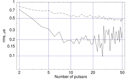
                           (b)

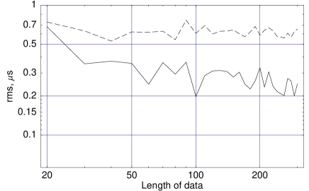
                           (c)

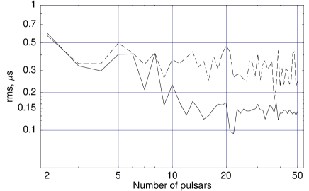
                           (d)

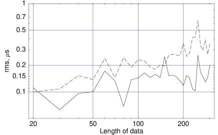
                           (e)

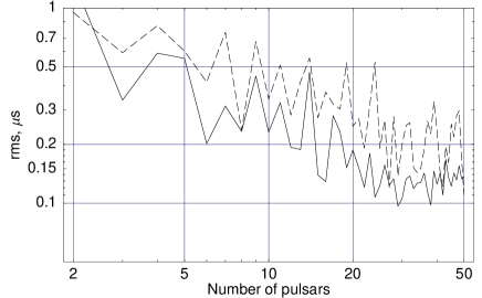
                           (f)

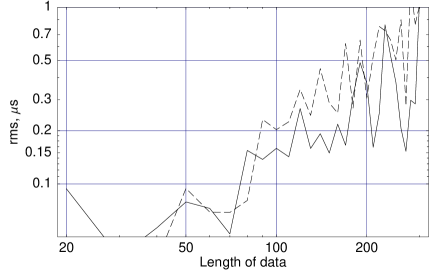
Figure 1: The accuracy of signal estimation based on the methods of weighted average (dashed line) and Wiener filter (solid line) as dependent on the number of pulsars (left panels) and length of the data (right panels). For the calculation shown in the left panels 256 points of data were taken, for calculations shown in the right panels five pulsars were used. Different types of noise were generated: (a), (b) - white phase noise, (c), (d) - white noise in frequency, (e), (f) - random walk noise in frequency. Data in the panels (d) and (f) were scaled accordingly for fitting within in all the panels.

To evaluate performance of the Wiener filtering method as compared to the weighted average method, we have applied it to simulated time sequences corresponding to harmonic signal with additive white and red (correlated) noise. Simulated time series were generated with the help of random generator built in the Mathematica software which had the preset (normal) distribution for different numbers of pulsars. A maximum of 50 pulsars were used (limited by acceptable computing time). The harmonic signal to be estimated was as follows: $A\sin(t/P)$, $A=1$, $P=10$, $t=1,2,\ldots,256$. The additive Gaussian white noise had zero mean and different variance. For example, in simulation for 50 pulsars, the variance was in the range of $\sigma^{2}=1,2,\ldots,50$. The correlated noise $n_{2},n_{4}$ with the power spectra $1/f^{2}$ and $1/f^{4}$ was generated as a single or twice repeated cumulative sum of the white noise $n_{0}$:

$$n_{2j}=\sum_{i=1}^{j}n_{0i},\;n_{4j}=\sum_{i=1}^{j}n_{2i},\;(j=1,2,\ldots,n).$$ (12)

The second order polynomial trend was subtracted from the generated time series $n_{2}$ and $n_{4}$. The weights of the individual time series were taken inversely proportional to $\sigma_{z}^{2}$, where $\sigma_{z}$ is the fractional instability [Taylor 1991]. Quality of the two methods was compared by calculating the root mean square of the difference between original and recovered signals.

Fig. 1 shows the results of computer simulation described above. Quality of these two methods of signal estimation is clearly visible. It is important to note that signal estimation accuracy in the case of Wiener filter (solid line) is better in all cases. The most significant advantage of the Wiener filter over the weighted average method is seen in the case of the white noise (fig. 1(a), 1(b)). For the correlated noise with the power spectrum $1/f^{2}$ (fig. 1(c), 1(d)) the advantage is still clear. For the red noise with the power spectrum $1/f^{4}$ both methods show similar results (fig. 1(e), 1(f)). Noteworthy is dependence of estimation quality on the observation interval for the correlated noise (fig. 1(d), 1(f)): as the observation interval increases, the estimation accuracy grows. Physically such a behaviour corresponds to appearance of more and more strong variations of the correlated noise with time, which deteriorate the signal estimation quality. Influence of the form of the correlated noise and length of the observation interval on the variances of the pulsar timing parameters are described in detail in [Kopeikin 1997].

5 Results

To evaluate the performance of the proposed Wiener filter method, timing data of pulsars PSR B1855+09 and B1937+21 [Kaspi, Taylor & Ryba 1994] were used. For the sake of simplicity of the subsequent matrix computations, unevenly spaced data were transformed into uniform ones with a sampling interval of 10 days by means of linear interpolation. Such a procedure perturbs a high-frequency component of the data while leaving a low-frequency component, of most interest to us, unchanged. The sampling interval of 10 days was chosen to preserve approximately the same volume of data.

The common part of the residuals for both pulsars (251 TOAs) has been taken within the interval $MJD=46450\div 48950$. Since choosing the common part of the time series changes the mean and slope, the residuals have been quadratically refitted for consistency with the classical timing fit. The pulsar post-fit timing residuals before and after processing described above are shown in Fig. 2.

                           (a)

                           (b)

Figure 2: The barycentric timing residuals of pulsars PSR B1855+09 (thin line) and PSR B1937+21 (solid line) before (a) and after (b) uniform sampling.

According to [Kaspi, Taylor & Ryba 1994], the timing data of PSRs B1855+09 and B1937+21 are in UTC time scale. UTC (Universal Coordinated Time) is the international atomic time scale that serves as the basis for timekeeping for most of the world. UTC runs at the same frequency as TAI (International Atomic Time). It differs from TAI by an integral number of seconds. This difference increases when so-called leap seconds occur. The purpose of adding leap seconds is to keep atomic time (UTC) within $\pm 0.9$ s of an time scale called UT1, which is based on the rotational rate of the Earth. Local realisations of UTC exist at the national time laboratories. These laboratories participate in the calculation of the international time scales by sending their clock data to the BIPM. The difference between UTC (computed by BIPM) and any other timing centre’s UTC only becomes known after computation and dissemination of UTC, which occurs about two weeks later. This difference is presently limited mainly by the long-term frequency instability of UTC [Audoin & Guinot 2001].

The signal we need to estimate is the difference UTC – PT. Fig. 3 shows the signal estimates (thin line) based on the timing residuals of pulsars PSR B1855+09 and PSR B1937+21 and calculated with use of eq. (4). The combined signal (ensemble pulsar time scale, eq. (7)) is shown in fig. 4 and displays behaviour similar to the difference UTC – TT(BIPM06) (correlation $\rho=0.75$).

                           (a)

                           (b)

Figure 3: Differences in UTC – PT₁₈₅₅ (a) and UTC – PT₁₉₃₇ (b) (thin line) for the interval $MJD=46450\div 48950$ estimated using the optimal filtering method (eq. (4)). The smoothing with Kaiser filter is shown by solid line. The dashed line displays the difference UTC – TT(BIPM06).

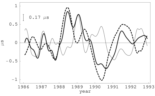
Figure 4: Combined clock variations of UTC – PT_ens for the interval $MJD=46450\div 48950$ estimated using the optimal filtering method from the timing residuals of pulsars PSR B1855+09 and PSR B1937+21 (solid line) and difference UTC – TT(BIPM06) (dashed line). The thin line indicates the difference TT – PT_ens

All three signals UTC – PT₁₈₅₅, UTC – PT₁₉₃₇ and UTC – PT_ens were smoothed by use of the following method: to decrease the Gibbs phenomenon (signal oscillations) near the ends of smoothing interval, the series under consideration were backward and forward forecasted by $p=IntegerPart[n/2]$ lags ($n=251$ is length of time series) with use of the Burg’s (also referred to as the maximum entropy method) autoregression algorithm of order $p$ [Burg, 1975, Terebizh 1992]. A new time series of double length were smoothed by use of the low-pass Kaiser filter [Gold & Rader 1973, Kaiser 1974] with the bandwidth of $f_{\rm max}/32$, where $f_{\rm max}=2/\Delta t$, $\Delta t=10$ days is the sampling interval. The choice of the bandwidth was defined by visual comparison with the UTC – TT(BIPM06) line. The final time series were obtained by dropping the forward and backward forecasted sections of the smoothed series.

The accuracy of the obtained realisations of the pulsar time UTC – PT₁₈₅₅ and UTC – PT₁₉₃₇ was derived from the diagonal elements of the covariance matrix defined by eq. (5). The root mean square value of UTC – PT₁₈₅₅ and UTC – PT₁₉₃₇ is equal to 0.44 $\mu$s and 0.67 $\mu$s respectively. The accuracy of the smoothed signals was estimated as $0.44/\sqrt{16}=0.11$ $\mu$s and $0.67/\sqrt{16}=0.17$ $\mu$s. Finally, for overall accuracy a conservative estimate 0.17 $\mu$s was accepted.

6 Discussion

The stability of a time scale is characterised by so-called Allan variance numerically expressed as a second-order difference of the clock phase variations. Since timing analysis usually includes determination of the pulsar spin parameters up to at least the first derivative of the rotational frequency, it is equivalent to excluding the second order derivative from pulsar TOA residuals and therefore there is no sense in the Allan variance. For this reason, for calculation of the fractional instability of a pulsar as a clock, another statistic $\sigma_{z}$ has been proposed [Taylor 1991]. A detailed numerical algorithm for calculation of $\sigma_{z}$ has been described in the paper [Matsakis, Taylor & Eubanks 1997].

In this work, an idea has been proven that different realisations of pulsar time scales must have comparable stability between each other [Lyne & Graham-Smith, 1998] and should be not worse than available terrestrial time scale at the same interval. For this purpose statistic $\sigma_{z}$ of two realisations of PT, UTC – PT₁₈₅₅ and UTC – PT₁₉₃₇, were compared.

Fig. 5 presents the fractional instability of the differences PT₁₉₃₇ – PT₁₈₅₅ (dashed line) and TT – PT_ens (solid line). At 7 years time interval $\sigma_{z}=(0.8\pm 1.9)\cdot 10^{-15}$ and $\sigma_{z}=(1.6\pm 2.9)\cdot 10^{-15}$ for TT – PT_ens and PT₁₉₃₇ – PT₁₈₅₅ respectively. One can see that instability of the two differences lays within error bar intervals. The fractional instability of TT relative to PT_ens and PT₁₉₃₇ relative to PT₁₈₅₅ is almost one order of magnitude better than individual fractional instability of the pulsars PSR B1855+09 and PSR B1937+21.

As an example of astrophysical application of the fractional instability values obtained in this work, one could consider estimation of the upper limit of the energy density of the stochastic gravitational wave background [Kaspi, Taylor & Ryba 1994]. For this purpose theoretical lines of $\sigma_{z}$ in the case when the gravitational wave background with the fractional energy density $\Omega_{g}h^{2}=10^{-9}$ and $10^{-10}$ begins to dominate are plotted in the lower right hand side corner of fig. 5. One can see that $\sigma_{z}$ of TT – PT_ens crosses the line $\Omega_{g}h^{2}=10^{-9}$ and approaches $\Omega_{g}h^{2}=10^{-10}$. The upper limit of $\Omega_{g}h^{2}$ based on the two sigma uncertainty (95% confidence level) of the ensemble $\sigma_{z}$ is equal to $\sim 3\cdot 10^{-9}$.

Noteworthy, that since PSRs 1855+09 and 1937+21 are relatively close to each other in the sky (angular separation is $15.5^{\circ}$) and hence their variations of the rotational phase contain a correlated contribution caused by the stochastic gravitational wave background [Hellings & Downs 1983], they form a good pair for estimation of the upper limit of $\Omega_{g}h^{2}$.

Currently, the accuracy of the filtering method without contribution of the uncertainty of the TT algorithm is estimated at a level of 0.17 $\mu$s. So, the uncertainty in PT_ens may, in principle, reach the level of a few ten nanoseconds if it were to be used for all high-stable millisecond pulsars. As computer simulations show, for the highest advantage while applying the Wiener optimal filters one should use the pulsars that show no correlated noise in their post-fit timing residuals.

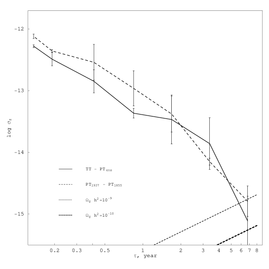
Figure 5: The fractional instability $\sigma_{z}$ based on the difference PT₁₉₃₇–PT₁₈₅₅ (dashed line) and $\sigma_{z}$ of the difference TT – PT_ens (solid line). Theoretical $\sigma_{z}$ in the case $\Omega_{g}h^{2}=10^{-9}$ and $10^{-10}$ are shown in the lower right-hand corner of the plot.

7 Conclusions

An algorithm of forming of ensemble pulsar time scale based on the method of the optimal Wiener filtering is presented. The basic idea of the algorithm consists in the use of optimal filter for removal of additive noise from the timing data before construction of the weighted average ensemble time scale.

Such a filtering approach offers an advantage over the weighted average algorithm since it utilises additional statistical information about common signal in the form of its covariance function or power spectrum. Since timing data are always available relative to a definite time scale, for separation of the pulsar and clock contributions one need to use observations from a few pulsars (minimum two) relative to the same time scale. Such approach allows estimation of the signal covariance function (power spectrum) by averaging all cross-covariance functions or power cross-spectra of the original data.

The availability of two scale differences UTC – TT and UTC – PT has resulted in the long awaited possibility of comparing the ultimate terrestrial time scale TT and extraterrestrial ensemble pulsar time scale PT of comparable accuracy. The fractional instability of the terrestrial time scale TT relative to PT and their high correlation have demonstrated that PT scale can be successfully used for monitoring the long-term variations of TT.

References

- [Audoin & Guinot 2001] Audoin C., Guinot B., 2001, The Measurement of Time, Cambridge University Press, 1st ed.
- [Backer et al. 1982] Backer D.C., Kulkarni S.R., Heiles C.E., Davis M.M., Goss W.M., 1982, Nature, 300, 615.
- [Backer & Hellings, 1986] Backer D.C., Hellings R.W., 1986, Ann. Rev. Astron. Astrophys., 24, 537-75.
- [Burg, 1975] Burg J.P., 1975, Maximum entropy spectral analysis, PhD thesis, Stanford univ.
- [Doroshenko & Kopeikin 1990] Doroshenko O.V., Kopeikin S.M., 1990, Sov.Astr., 34, 245.
- [Edwards, Hobbs & Manchester 2006] Edwards, R. T., Hobbs, G. B., Manchester, R. N., 2006, MNRAS, 372, 1549.
- [1990] Foster R.S., Backer D.C., 1990, ApJ, 361, 300.
- [Gold & Rader 1973] Gold B., Rader C.M., 1973, Digital Processing of Signals (with chapter by J. Kaiser ”Digital Filters”), Moscow: Sov.Radio (in Rissian).
- [Gubanov 1997] Gubanov V.S., 1997, Generalized least-squares. Theory and application in astrometry, S-Petersburg: Nauka (in Russian).
- [Guinot 1988] Guinot B., 1988, A&A, 192, 370.
- [Guinot & Petit 1991] Guinot B., Petit G., 1991, A&A, 248, 292.
- [Hellings & Downs 1983] Hellings R.W., Downs G.S., 1983, ApJ, 265, L39.
- [Hewish et al. 1968] Hewish A., Bell S.J., Pilkington J.D.H., Scott P.F., Collinset R.A., 1968, Nature, 217, 709.
- [1989] Ilyasov Yu.P., Kuzmin A.D., Shabanova T.V., Shitov Yu.P., 1989, FIAN proceedings, 199, 149.
- [Ilyasov et al. 1996] Ilyasov Yu., Imae M., Kopeikin S., Rodin A., Fukushima T., 1996, in: Modern problems and methods of astrometry and geodynamics, Finkelstein A. (ed.), S-Peterburg, p.143.
- [Ilyasov, Kopeikin & Rodin 1998] Ilyasov Yu.P., Kopeikin S.M., Rodin A.E., 1998, Astr.L., 24, 228.
- [Kaiser 1974] Kaiser J.F., 1974, Proc. 1974 IEEE Int. Symp. Circuit Theory, 20.
- [Kaspi, Taylor & Ryba 1994] Kaspi V.M., Taylor J.H., Ryba M.F., 1994, ApJ, 428, 713.
- [Kopeikin 1997] Kopeikin S.M., 1997, MNRAS, 288, 129.
- [Kopeikin 1999] Kopeikin S.M., 1999, MNRAS, 305, 563.
- [Lyne & Graham-Smith, 1998] Lyne A.G., Graham-Smith F., 1998, Pulsar Astronomy, Cambridge University Press; 2nd ed.
- [Matsakis, Taylor & Eubanks 1997] Matsakis D.N., Taylor J.H., Eubanks T.M., 1997, A&A, 326, 924.
- [Murray, 1986] Murray C. A., 1983, Vectorial Astrometry, Adam Hilger, Bristol.
- [Percival 1991] Percival D., 1991, Proc. IEEE, 79, 961.
- [1996] Petit G., Tavella P., A&A, 1996, 308, 290.
- [Rodin, Kopeikin & Ilyasov 1997] Rodin A.E., Kopeikin S.M., Ilyasov Yu.P., 1997, Acta Cosmologica, XXIII-2, 163.
- [Rodin 2006] Rodin A.E., 2006, Chin. J. Astron. Astrophys., 6, Suppl.2, 157.
- [Taylor 1991] Taylor J.H., 1991, Proc.IEEE, 79, 1054.
- [Terebizh 1992] Terebizh V.Yu., 1992, Time Series Analysis in Astrophysics, Moscow: Nauka (in Russian).
- [Wiener 1949] Wiener N., 1949, Extrapolation, Interpolation and Smoothing of Stationary Time Series, New York: Wiley.