KEK-CP-213
KEK Preprint 2008-13
MPP-2008-41
PSI-PR-08-07

NLO QCD corrections to ${\mathrm{t}}\bar{\mathrm{t}}{\mathrm{b}}\bar{\mathrm{b}}$ production
at the LHC: 1. quark–antiquark annihilation

A. Bredenstein¹, A. Denner², S. Dittmaier³ and S. Pozzorini³

¹ High Energy Accelerator Research Organization (KEK),
Tsukuba, Ibaraki 305-0801, Japan

² Paul Scherrer Institut, Würenlingen und Villigen,
CH-5232 Villigen PSI, Switzerland

³ Max-Planck-Institut für Physik (Werner-Heisenberg-Institut),
D-80805 München, Germany

Abstract:

The process ${\mathrm{p}}{\mathrm{p}}\to{\mathrm{t}}\bar{\mathrm{t}}{\mathrm{b}}\bar{\mathrm{b}}+X$ represents a very important background reaction to searches at the LHC, in particular to ${\mathrm{t}}\bar{\mathrm{t}}{\mathrm{H}}$ production where the Higgs boson decays into a ${\mathrm{b}}\bar{\mathrm{b}}$ pair. A successful analysis of ${\mathrm{t}}\bar{\mathrm{t}}{\mathrm{H}}$ at the LHC requires the knowledge of direct ${\mathrm{t}}\bar{\mathrm{t}}{\mathrm{b}}\bar{\mathrm{b}}$ production at next-to-leading order in QCD. We take the first step in this direction upon calculating the next-to-leading-order QCD corrections to the subprocess initiated by $q\bar{q}$ annihilation. We devote an appendix to the general issue of rational terms resulting from ultraviolet or infrared (soft or collinear) singularities within dimensional regularization. There we show that, for arbitrary processes, in the Feynman gauge, rational terms of infrared origin cancel in truncated one-loop diagrams and result only from trivial self-energy corrections.

July 2008

1 Introduction

The search for new particles will be the primary task of the LHC experiment at CERN starting this year. The discovery of new particles in the first place requires to establish excess of events over background. The situation at the LHC is particularly complicated by the fact that for many expected signals the corresponding background cannot entirely be determined from data, but has to be assessed upon combining measurements in signal-free regions with theory-driven extrapolations. To this end, a precise prediction for the background is necessary, in particular including next-to-leading-order (NLO) corrections in QCD. Since many of these background processes involve three, four, or even more particles in the final state, this kind of background control requires NLO calculations at the technical frontier. This problem lead to the creation of an “experimenters’ wishlist for NLO calculations” at the Les Houches workshop 2005 [1], updated in 2007 [2], which triggered great theoretical progress in recent years (see for instance Refs. [1, 2, 3, 4, 5, 6, 7, 8, 9, 10, 11, 12, 13, 14, 15] and references therein). Meanwhile the listed processes involving at most five particles in loops have been completed in NLO QCD, including the production of ${\mathrm{W}}{\mathrm{W}}+\mathrm{jet}$ [16, 17], weak-boson pairs plus two jets via vector-boson fusion [18], and triple weak-boson production [9, 19]. However, none of the true $2\to 4$ processes has yet been addressed at NLO. Among those processes, ${\mathrm{p}}{\mathrm{p}}\to{\mathrm{t}}\bar{\mathrm{t}}{\mathrm{b}}\bar{\mathrm{b}}+X$ has top priority. This process has also been discussed as signal of strong electroweak symmetry breaking [21].

The process of ${\mathrm{t}}\bar{\mathrm{t}}{\mathrm{b}}\bar{\mathrm{b}}$ production represents a very important background to ${\mathrm{t}}\bar{\mathrm{t}}{\mathrm{H}}$ production where the Higgs boson decays into a ${\mathrm{b}}\bar{\mathrm{b}}$ pair. While early studies of ${\mathrm{t}}\bar{\mathrm{t}}{\mathrm{H}}$ production at ATLAS [22] and CMS [23] suggested even discovery potential of this process for a light Higgs boson, more recent analyses [24, 25] with more realistic background assessments show that the signal significance is jeopardized if the background from ${\mathrm{t}}\bar{\mathrm{t}}{\mathrm{b}}\bar{\mathrm{b}}$ and ${\mathrm{t}}\bar{\mathrm{t}}+\mathrm{jets}$ final states is not controlled very well. This is a clear call for improved signal and background studies based on NLO predictions to these complicated processes. For the ${\mathrm{t}}\bar{\mathrm{t}}{\mathrm{H}}$ signal [26, 27] and the ${\mathrm{t}}\bar{\mathrm{t}}+\mathrm{1jet}$ background [28] at the LHC such predictions have been accomplished in recent years.

The dominant mechanism to produce ${\mathrm{t}}\bar{\mathrm{t}}{\mathrm{b}}\bar{\mathrm{b}}$ final states in hadronic collisions is pure QCD. In leading order (LO) quark–antiquark ($q\bar{q})$ and gluon–gluon (${\mathrm{g}}{\mathrm{g}}$) initial states contribute, where the latter strongly dominate at the LHC because of the high gluon flux. Being of order $\alpha^{4}_{\mathrm{s}}$ the corresponding cross sections are affected by a very large scale uncertainty, which amounts to a factor two or more. Technically the $q\bar{q}$ channel is simpler to deal with—though still demanding—and thus represents a natural first step towards a full treatment of ${\mathrm{p}}{\mathrm{p}}\to{\mathrm{t}}\bar{\mathrm{t}}{\mathrm{b}}\bar{\mathrm{b}}+X$ at NLO. In this paper we report on this first step and present some details of the calculation as well as numerical results. These results do not yet significantly improve the predictions for the LHC, but on the one hand form a building block of the full calculation and can serve as benchmark results for other groups on the other. Moreover, this step proves the performance of the applied strategy and methods, providing confidence that the more complicated ${\mathrm{g}}{\mathrm{g}}$ channel can be attacked widely in the same way.

In Section 2 we give a brief description of the NLO calculation, followed by numerical results on integrated cross sections in Section 3. Appendix A provides a general discussion of rational terms in one-loop amplitudes, and Appendix B outlines some technical details concerning our treatment of the Dirac algebra. Finally, as a benchmark, in Appendix C we give numerical results for the matrix element squared in lowest order and including virtual corrections for one phase-space point.

2 Details of the calculation

In LO QCD seven different Feynman diagrams contribute to the partonic process $q\bar{q}\to{\mathrm{t}}\bar{\mathrm{t}}{\mathrm{b}}\bar{\mathrm{b}}$; the various topologies are shown in Figure 1.

0.8    

Figure 1: Two different diagram topologies contributing to $q\bar{q}\to{\mathrm{t}}\bar{\mathrm{t}}{\mathrm{b}}\bar{\mathrm{b}}$ in LO QCD; there are six explicit diagrams of the first and one of the second kind.

The virtual QCD corrections comprise about 200 one-loop diagrams, the most complicated being the 8 hexagons and 24 pentagons, which are illustrated in Figure 2.

0.8    

Figure 2: Diagram topologies for pentagon and hexagon graphs contributing to $q\bar{q}\to{\mathrm{t}}\bar{\mathrm{t}}{\mathrm{b}}\bar{\mathrm{b}}$ at one loop in QCD; there are 24 explicit pentagons and 8 hexagons.

The real QCD corrections in the $q\bar{q}$ channel are induced by gluon bremsstrahlung, $q\bar{q}\to{\mathrm{t}}\bar{\mathrm{t}}{\mathrm{b}}\bar{\mathrm{b}}{\mathrm{g}}$, where the corresponding 64 diagrams are obtained from the LO graphs upon adding an external gluon in all possible ways. In the following we briefly describe the calculation of the virtual and real corrections, where each of these contributions has been worked out twice and independently, resulting in two completely independent computer codes.

2.1 Virtual corrections

The general strategy for the evaluation of the one-loop corrections is based on the reduction of the amplitude ${\cal{M}}^{(\Gamma)}$ of each (sub)diagram $\Gamma$ in the following way,

$${\cal{M}}^{(\Gamma)}={\cal C}^{(\Gamma)}\left(\sum_{m}{\cal F}^{(\Gamma)}_{m}(\{(p_{a}p_{b})\})\,\hat{\cal{M}}_{m}(\{p_{a}\})\right),$$ (2.1)

where the colour structure ${\cal C}^{(\Gamma)}$ present in the (sub)diagram is factorized from the remaining colour-independent part. The decomposition of the colour structure,

$${\cal C}^{(\Gamma)}=\sum_{k=1}^{6}c^{(\Gamma)}_{k}{\cal C}_{k},$$ (2.2)

is done in a basis $\{{\cal C}_{k}\}$ consisting of six elements, which can be chosen as

$${\cal C}_{1}=1\otimes T^{a}\otimes T^{a},\qquad{\cal C}_{2}=T^{a}\otimes 1\otimes T^{a},\qquad{\cal C}_{3}=T^{a}\otimes T^{a}\otimes 1,$$ (2.3)

$${\cal C}_{4}=1\otimes 1\otimes 1,\qquad{\cal C}_{5}=f^{abc}\,T^{a}\otimes T^{b}\otimes T^{c},\qquad{\cal C}_{6}=d^{abc}\,T^{a}\otimes T^{b}\otimes T^{c}.$$

Here $T^{a}$, $f^{abc}$, $d^{abc}$ are the usual SU(3) objects, and the tensor products connect the three fermionic chains. The LO amplitude is decomposed in colour space as

$${\cal{M}}^{{\mathrm{LO}}}=\sum_{l=1}^{6}{\cal C}_{l}\,{\cal M}^{{\mathrm{LO}}}_{l}.$$ (2.4)

In general each loop diagram gives rise to $3^{n_{4}}$ colour-factorized amplitudes of type (2.1), where $n_{4}$ is the number of quartic gluon vertices in the diagram. However, for most diagrams $n_{4}=0$, and the colour structure factorizes completely. The colour separation implies that the computation time for individual loop diagrams does not scale with the number of colour structures present in the basis $\{{\cal C}_{k}\}$.

The colour-free parts of ${\cal{M}}^{(\Gamma)}$ are written as a linear combination of so-called standard matrix elements (SMEs) $\hat{\cal{M}}_{m}(\{p_{a}\})$, which contain all Dirac chains and the polarization information. Since the computing time scales with the number of SMEs, it is important to reduce the set of SMEs $\{\hat{\cal{M}}_{m}\}$ as much as possible. To this end, we employ an algebraic procedure based on four-dimensional relations that are derived from Chisholm’s identity whenever their use is admitted. For massless external fermions this four-dimensional reduction has been described in detail in Sections 3.1 and 3.3 of Ref. [29]; here we had to generalize this approach to one massive and two massless spinor chains. In this way some thousand different spinor chains are reduced to about 150 SMEs $\hat{\cal{M}}_{m}(\{p_{a}\})$. A brief description of this procedure, which is implemented in two independent Mathematica programs, is outlined in App. B.

The one-loop correction to the spin- and colour-summed squared amplitude induced by $\Gamma$ reads

$$2\mathop{\mathrm{Re}}\nolimits\,\Biggl{\{}\sum_{\mathrm{col}}\sum_{\mathrm{pol}}{\cal{M}}^{(\Gamma)}\left({\cal{M}}^{{\mathrm{LO}}}\right)^{*}\Biggr{\}}=2\mathop{\mathrm{Re}}\nolimits\,\left\{\sum_{k=1}^{6}c^{(\Gamma)}_{k}\sum_{m}{\cal F}^{(\Gamma)}_{m}(\{(p_{a}p_{b})\})\,M_{km}(\{(p_{a}p_{b})\})\right\},$$ (2.5)

where the interference of the LO amplitude with the elements of the SME and colour basis,

$$M_{km}(\{(p_{a}p_{b})\}) = \sum_{\mathrm{col}}{\cal C}_{k}\sum_{\mathrm{pol}}\hat{\cal{M}}_{m}(\{p_{a}\})\left({\cal{M}}^{{\mathrm{LO}}}\right)^{*}$$ (2.6)

$$= \sum_{l}\sum_{\mathrm{col}}{\cal C}_{k}{\cal C}^{*}_{l}\sum_{\mathrm{pol}}\hat{\cal{M}}_{m}(\{p_{a}\})\left({\cal{M}}_{l}^{{\mathrm{LO}}}\right)^{*},$$

has to be calculated only once per phase-space point. Moreover, the colour-correlation matrix $\sum_{\mathrm{col}}{\cal C}_{k}{\cal C}^{*}_{l}$ obviously is independent of the kinematics and is only calculated once and for all. The most time-consuming components of the numerical calculation are the scalar form factors ${\cal F}^{(\Gamma)}_{m}$, which are linear combinations of the Lorentz-invariant coefficients of $N$-point tensor loop integrals with rank $R\leq 3$ and degree $N\leq 6$,

$${\cal F}^{(\Gamma)}_{m}(\{(p_{a}p_{b})\})=\sum_{R}\,\sum_{j_{1},\dots,j_{R}}{\cal K}^{(\Gamma)}_{m;j_{1},\dots,j_{R}}(\{(p_{a}p_{b})\})\,T^{N}_{j_{1},\dots,j_{R}}(\{(p_{a}p_{b})\}).$$ (2.7)

The evaluation of one-loop tensor integrals $T^{N}_{j_{1},\dots,j_{R}}$ follows the strategy of Refs. [4, 5] that was already successfully used to compute the NLO electroweak corrections to ${\mathrm{e^{+}}}{\mathrm{e^{-}}}\to 4\,$fermions [29, 31]. In this approach the analytic expressions are not reduced to master integrals. In contrast, the tensor integrals are evaluated by means of algorithms that perform a recursive reduction to master integrals in numerical form. This avoids huge analytic expressions and permits to adapt the reduction strategy to the specific numerical problems that appear in different phase-space regions.

The scalar master integrals are evaluated using the methods and results of Refs. [32, 33]. Ultraviolet (UV) divergences are regularized dimensionally in both evaluations, but infrared (IR) divergences are treated in different ways as described below. Following ideas from the 1960’s [34], tensor and scalar 6-/5-point functions are directly expressed in terms of 5-/4-point integrals [4, 5]. Tensor 4-point and 3-point integrals are reduced to scalar integrals with the Passarino–Veltman algorithm [35] as long as no small Gram determinant appears in the reduction. If small Gram determinants occur, two alternative schemes are applied [5]. One method makes use of expansions of the tensor coefficients about the limit of vanishing Gram determinants and possibly other kinematical determinants. In the second (alternative) method we evaluate a specific tensor coefficient, the integrand of which is logarithmic in Feynman parametrization, by numerical integration. Then the remaining coefficients as well as the standard scalar integral are algebraically derived from this coefficient. The results of the two different codes, based on the different methods described above are in good numerical agreement. Although both versions of the virtual corrections basically follow the same strategy for the evaluation of loop integrals, they are based on independent in-house libraries. In each of the two calculations the cancellation of IR and UV singularities was checked with high precision in the numerical results.

Version 1 of the virtual corrections starts with the generation of Feynman diagrams using FeynArts 1.0 [36]. Their algebraic reduction is completely performed with in-house Mathematica routines. In detail, $D$-dimensional identities (Dirac algebra, Dirac equation) are used until UV divergences cancel against counterterms. IR (soft and collinear) divergences are regularized dimensionally and separated from full diagrams in terms of 3-point subdiagrams as described in Ref. [37]. We subtract the IR-divergent part ${\cal{M}}^{(\Gamma,D)}_{\mathrm{sing}}$ from the amplitude ${\cal{M}}^{(\Gamma,D)}$ of a (sub-)diagram $\Gamma$, where $D$ indicates dimensional regularization, and add it back. Note that ${\cal{M}}^{(\Gamma,D)}_{\mathrm{sing}}$ can be easily constructed already at the integrand level of the whole diagram following Ref. [37]. In the IR-finite and regularization-scheme-independent difference ${\cal{M}}^{(\Gamma,D)}-{\cal{M}}^{(\Gamma,D)}_{\mathrm{sing}}$ we can then switch from dimensional regularization to a four-dimensional scheme,

$${\cal{M}}^{(\Gamma,D)}=\left({\cal{M}}^{(\Gamma,D)}-{\cal{M}}^{(\Gamma,D)}_{\mathrm{sing}}\right)+{\cal{M}}^{(\Gamma,D)}_{\mathrm{sing}}=\left({\cal{M}}^{(\Gamma,\lambda)}-{\cal{M}}^{(\Gamma,\lambda)}_{\mathrm{sing}}\right)+{\cal{M}}^{(\Gamma,D)}_{\mathrm{sing}},$$ (2.8)

where $\lambda$ indicates any mass regulators in four dimensions. Specifically, we introduce infinitesimal light-quark and gluon masses with the hierarchy $m_{\mathrm{g}}\ll m_{q}$ to regularize the IR singularities. The evaluation of ${\cal{M}}^{(\Gamma,\lambda)}$ then proceeds in $D=4-2\epsilon$ dimension merely to regularize the UV singularities, i.e. so-called rational terms resulting from $(D-4)$ times poles in $\epsilon$ have to be taken care of for UV singularities, but not for IR singularities in this part. Possible rational terms of IR origin are contained in ${\cal{M}}^{(\Gamma,D)}_{\mathrm{sing}}$ which entirely consists of 3-point subgraphs and is thus easy to reduce to scalar 2- and 3-point integrals $B_{0}$ and $C_{0}$, thereby keeping the full dependence on $D$. It turns out that no $D$-dependent prefactors occur in front of IR-singular integrals. In App. A we show that this result of our specific calculation is not accidental, but generalizes to arbitrary processes at NLO. Technically it is easier to evaluate ${\cal{M}}^{(\Gamma,D)}_{\mathrm{sing}}$ and ${\cal{M}}^{(\Gamma,\lambda)}_{\mathrm{sing}}$ simultaneously according to

$${\cal{M}}^{(\Gamma,D)}_{\mathrm{sing}}-{\cal{M}}^{(\Gamma,\lambda)}_{\mathrm{sing}}={\cal{M}}^{(\Gamma,D)}_{\mathrm{sing}}\Big{|}_{B_{0}^{(D)}\to\Delta B_{0},C_{0}^{(D)}\to\Delta C_{0}}\equiv\Delta{\cal{M}}^{(\Gamma)}_{\mathrm{sing}},$$ (2.9)

where $\Delta I=I^{(D)}-I^{(\lambda)}$ are the differences of the scalar integrals $I=B_{0},C_{0}$ in the two IR regularization schemes. Note that IR-finite integrals drop out in $\Delta{\cal{M}}^{(\Gamma)}_{\mathrm{sing}}$ completely. Having cancelled UV divergences against counterterms and controlled the $D$-dimensional issues concerning IR singularities, the amplitude is further simplified in four space–time dimensions. Specifically, the reduction of SMEs described in App. B is performed then. The IR-divergent “endpoint part” of the dipole subtraction function, i.e. the contribution of the $I$ operator as defined in Ref. [38], is processed through the described algebraic manipulations in the same way as LO and one-loop amplitudes. The algebraic Mathematica output of each diagram is automatically processed to Fortran for the numerical evaluation.

Version 2 of the virtual corrections employs FeynArts 3.2 [39] for generating and FormCalc 5.2 [40] for preprocessing the amplitudes. The first part of the calculation is performed in $D$ dimensions. In particular, the so-called rational terms resulting from the UV divergences of tensor loop coefficients are automatically extracted by FormCalc. Since the IR divergences that appear in the $q\bar{q}$ channel are of abelian nature, we exploit the fact that they can be regularized as in QED by means of fermion and gauge-boson (gluon) masses, $m_{q}$ and $m_{\mathrm{g}}$. These masses are treated as infinitesimal quantities (with $m_{\mathrm{g}}\ll m_{q}$) both in the algebraic expressions and in the numerical routines that evaluate the tensor integrals, i.e. only the logarithmic dependence on these mass parameters is retained. Corresponding IR singularities associated with real emission have been obtained from Ref. [38] by means of an appropriate change of regularization scheme.

Being of diagrammatic nature, the employed techniques are sometimes denoted as “brute force” methods. This choice of the terminology might suggest scarce efficiency. In fact, the performance of the algorithms is a very important issue that should be assessed by means of those quantities that describe the problematic aspects of NLO multi-leg calculations: numerical accuracy and CPU time. In this respect our treatment of the virtual corrections is characterized by high numerical precision and speed. The numerical agreement between the two programs is good, and the CPU time needed to evaluate a phase-space point (including sums over colours and polarizations) amounts to about $10^{-2}$ seconds on a single 3 GHz Intel Xeon processor. This provides a benchmark that can be compared with the efficiency of other approaches.

2.2 Real corrections

In both evaluations of the real corrections the amplitudes are calculated in the form of helicity matrix elements. The singularities for soft or collinear gluon emission are isolated via dipole subtraction [38, 41, 42, 43] for NLO QCD calculations using the formulation [38] for massive quarks. After combining virtual and real corrections, singularities connected to collinear configurations in the final state cancel for “collinear-safe” observables automatically after applying a jet algorithm, singularities connected to collinear initial-state splittings are removed via $\overline{\mathrm{MS}}$ QCD factorization by PDF redefinitions. While soft and collinear singularities have to be regularized in the “endpoint part” of the subtraction function, i.e. the part of the subtraction terms that has to be combined with the virtual corrections, no regularization is needed in the subtraction terms for the real corrections. In both evaluations the phase-space integration is performed with multichannel Monte Carlo generators [44] and adaptive weight optimization similar to the one implemented in RacoonWW [45].

In version 1 of the real corrections the matrix elements have been calculated using the Weyl–van-der-Waerden spinor technique in the formulation of Ref. [46]. Soft and collinear singularities are regularized using dimensional regularization. The phase-space integration, implemented in C++, is based on RacoonWW, but the phase-space mappings are built up in a more generic way very similar to the approach of Lusifer [47].

In version 2 of the real corrections the matrix elements have been generated with Madgraph 4.1.33 [48]. As in the corresponding virtual corrections, soft singularities are regularized by an infinitesimal gluon mass and collinear singularities by small quark masses, which appear only in logarithms in the endpoint part of the subtraction function. The Monte Carlo generator is a further development of the one used in COFFER$\gamma\gamma$ [49] and for the calculation of the NLO corrections to ${\mathrm{p}}{\mathrm{p}}\to{\mathrm{H}}+\mathrm{2jets}+X$ [50].

In version 2 we have also implemented two-cut-off slicing for the purpose of checking. In this approach (as e.g. reviewed in Ref. [51]), phase-space regions where real gluon emission contains soft or collinear singularities are defined by the auxiliary cutoff parameters $\delta_{\mathrm{s}},\;\delta_{\mathrm{c}}\ll 1$ in the partonic centre-of-mass frame. In real gluon radiation processes, the region

$$m_{\mathrm{g}}<k^{0}<\delta_{\mathrm{s}}\frac{\sqrt{\hat{s}}}{2},$$ (2.10)

where $k$ is the gluon momentum and $\sqrt{\hat{s}}$ the partonic centre-of-mass energy, is treated in soft approximation. The regions determined by

$$1-\cos(\theta_{{\mathrm{g}}q})<\delta_{\mathrm{c}},\qquad k^{0}>\delta_{\mathrm{s}}\frac{\sqrt{\hat{s}}}{2},$$ (2.11)

where $\theta_{{\mathrm{g}}q}$ is the angle between any light quark $q$ (including b quarks) and the gluon, are evaluated using collinear factorization. We again use an infinitesimal gluon mass and quark masses as regulators. In this regularization the contributions of the soft regions for light quarks and of the collinear regions can be found in Ref. [52], and the contributions of the soft regions involving top quarks can easily be calculated with the explicit results for the soft integrals in Refs. [32, 53]. In the remaining phase space no regulators are used. When adding all contributions, the dependence on the technical cuts cancels if the cut-off parameters are chosen to be small enough so that the soft and collinear approximations apply, i.e. the slicing result is correct up to terms of ${\cal O}(\delta_{\mathrm{s}})$ and ${\cal O}(\delta_{\mathrm{c}})$. Since the numerical cancellations between the different contributions grow with smaller cut parameters, the numerical error blows up if these parameters are too small.

3 Numerical results

We consider the process ${\mathrm{p}}{\mathrm{p}}\to{\mathrm{t}}\bar{\mathrm{t}}{\mathrm{b}}\bar{\mathrm{b}}+X$ at the LHC, i.e. for $\sqrt{s}=14\,\mathrm{TeV}$. For the top-quark mass, renormalized in the on-shell scheme, we take the numerical value $m_{\mathrm{t}}=172.6\,\mathrm{GeV}$ [54]. All other QCD partons (including ${\mathrm{b}}$ quarks) are treated as massless particles, and collinear final-state configurations, which give rise to singularities, are recombined into IR-safe jets using a $k_{{\mathrm{T}}}$-algorithm [55]. Specifically, we adopt the $k_{\mathrm{T}}$-algorithm of Ref. [56] and recombine all final-state b quarks and gluons with pseudorapidity $|\eta|<5$ into jets with separation $\sqrt{\Delta\phi^{2}+\Delta y^{2}}>D=0.8$ in the rapidity–azimuthal-angle plane. Requiring two b-quark jets, this also avoids collinear singularities resulting from the splitting of gluons into (massless) b quarks. Motivated by the search for a ${\mathrm{t}}\bar{\mathrm{t}}H(H\to{\mathrm{b}}\bar{\mathrm{b}})$ signal at the LHC [24, 25], we impose the following additional cuts on the transverse momenta, the rapidity, and the invariant mass of the two (recombined) b-jets: $p_{{\mathrm{T}},{\mathrm{b}}}>20\,\mathrm{GeV}$, $|y_{\mathrm{b}}|<2.5$, and $m_{{\mathrm{b}}\bar{\mathrm{b}}}>m_{{\mathrm{b}}\bar{\mathrm{b}},\mathrm{cut}}$. We plot results either as a function of $m_{{\mathrm{b}}\bar{\mathrm{b}},\mathrm{cut}}$ or for $m_{{\mathrm{b}}\bar{\mathrm{b}},\mathrm{cut}}=0$. Note, however, that the jet algorithm and the requirement of having two b jets with $p_{{\mathrm{T}},{\mathrm{b}}}>20\,\mathrm{GeV}$ in the final state sets an effective lower limit on the invariant mass $m_{{\mathrm{b}}\bar{\mathrm{b}}}$ of roughly $20\,\mathrm{GeV}$. The outgoing (anti)top quarks are neither affected by the jet algorithm nor by phase-space cuts.

We consistently use the CTEQ6 [57] set of parton distribution functions (PDFs), i.e. we take CTEQ6L1 PDFs with a 1-loop running $\alpha_{\mathrm{s}}$ in LO and CTEQ6M PDFs with a 2-loop running $\alpha_{\mathrm{s}}$ in NLO, but the suppressed contribution from b quarks in the initial state has been neglected. The number of active flavours is $N_{\mathrm{F}}=5$, and the respective QCD parameters are $\Lambda_{5}^{\mathrm{LO}}=165\,\mathrm{MeV}$ and $\Lambda_{5}^{\overline{\mathrm{MS}}}=226\,\mathrm{MeV}$. In the renormalization of the strong coupling constant the top-quark loop in the gluon self-energy is subtracted at zero momentum. In this scheme the running of $\alpha_{\mathrm{s}}$ is generated solely by the contributions of the light-quark and gluon loops. This yields $\alpha_{\mathrm{s}}(m_{\mathrm{t}})|_{\mathrm{LO}}=0.1178730\ldots$ and $\alpha_{\mathrm{s}}(m_{\mathrm{t}})|_{\mathrm{NLO}}=0.1076396\ldots$. By default, we set the renormalization and factorization scales, $\mu_{\mathrm{R}}$ and $\mu_{\mathrm{F}}$, to the common value $\mu_{0}=m_{\mathrm{t}}+m_{{\mathrm{b}}\bar{\mathrm{b}},\mathrm{cut}}/2$.

3.1 Integrated cross sections

We first consider results for integrated cross sections. Figure 3 shows the total LO cross section and the contribution induced by $q\bar{q}$ annihilation at the LHC as a function of $m_{{\mathrm{b}}\bar{\mathrm{b}},\mathrm{cut}}$.

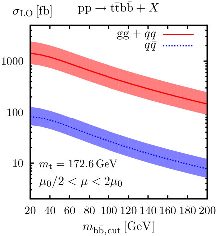
Figure 3: LO cross section (${\mathrm{g}}{\mathrm{g}}+q\bar{q}$) versus contribution from $q\bar{q}$ annihilation for ${\mathrm{p}}{\mathrm{p}}\to{\mathrm{t}}\bar{\mathrm{t}}{\mathrm{b}}\bar{\mathrm{b}}+X$ at the LHC as function of the cut $m_{{\mathrm{b}}\bar{\mathrm{b}},\mathrm{cut}}$ on the invariant mass of the ${\mathrm{b}}\bar{\mathrm{b}}$ pair.

For the chosen setup ${\mathrm{g}}{\mathrm{g}}$ fusion dominates over the $q\bar{q}$ channel by roughly a factor 17. The renormalization and factorization scale dependence of the LO prediction is indicated by bands resulting from varying the central scale $\mu_{0}$ up and down by a factor 2 which corresponds to a variation of the cross section by a factor 1.6. Owing to the large power of $\alpha_{\mathrm{s}}(\mu_{\mathrm{R}})^{4}$ in the LO cross section the scale uncertainty is strongly dominated by the renormalization scale dependence. We note that the LO cross sections have also been reproduced with the program Sherpa [58].

Figure 4 illustrates the mutual agreement between NLO results obtained with dipole subtraction and two-cutoff phase-space slicing.

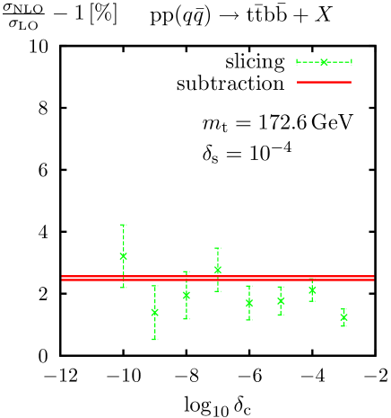
Figure 4: Comparison of the relative NLO corrections to ${\mathrm{p}}{\mathrm{p}}(q\bar{q})\to{\mathrm{t}}\bar{\mathrm{t}}{\mathrm{b}}\bar{\mathrm{b}}+X$ at the LHC as obtained with dipole subtraction and two-cutoff phase-space slicing using $m_{{\mathrm{b}}\bar{\mathrm{b}},\mathrm{cut}}=0$ and $\mu_{\mathrm{R}}=\mu_{\mathrm{F}}=\mu_{0}=m_{\mathrm{t}}$.

We find that within integration errors the slicing results become independent of the cut-offs for $\delta_{\mathrm{s}}\mathrel{\raisebox{-3.00003pt}{$\stackrel{{\scriptstyle\displaystyle<}}{{\sim}}$}}10^{-3}$ and $\delta_{\mathrm{c}}\mathrel{\raisebox{-3.00003pt}{$\stackrel{{\scriptstyle\displaystyle<}}{{\sim}}$}}10^{-4}$ and agree nicely with the result of the subtraction method. While the latter has been obtained with $2\times 10^{8}$ events, the slicing results are based on $10^{9}$ events. Still the statistical error obtained with the subtraction approach (indicated by the width of the band) is almost an order of magnitude smaller than its slicing counterpart (errorbars), demonstrating the higher efficiency of dipole subtraction. The results shown in the following are obtained with the subtraction approach.

In Figure 5 we show the scale dependence of the LO and NLO cross sections induced by the $q\bar{q}$ channel upon varying the renormalization and factorization scales in a uniform or an antipodal way.

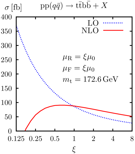
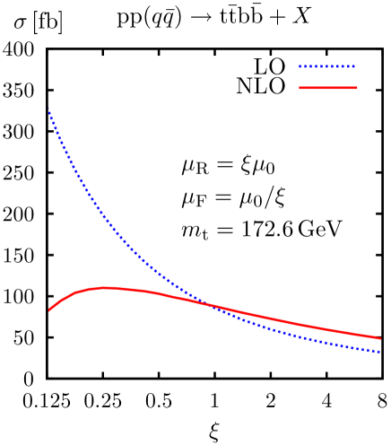
Figure 5: Dependence of the LO and NLO cross sections of ${\mathrm{p}}{\mathrm{p}}(q\bar{q})\to{\mathrm{t}}\bar{\mathrm{t}}{\mathrm{b}}\bar{\mathrm{b}}+X$ at the LHC for $m_{{\mathrm{b}}\bar{\mathrm{b}},\mathrm{cut}}=0$ and $\mu_{0}=m_{\mathrm{t}}$.

We observe a sizeable reduction of the scale uncertainty upon going from LO to NLO. Varying the scale up and down by a factor 2 changes the cross section by 55% in LO and by 17% in NLO. At the central scale, the NLO correction is small, i.e. $\sim 2.5\%$, and the LO and NLO cross sections are given by $\sigma_{\mathrm{LO}}=85.522(26)\,\mathrm{fb}$ and $\sigma_{\mathrm{NLO}}=87.698(56)\,\mathrm{fb}$. The numbers in parentheses are the errors of the Monte Carlo integration for $2\times 10^{8}$ events, where the virtual corrections are only calculated for each 5th event.

Figure 6 shows the LO and NLO cross sections as function of the cut $m_{{\mathrm{b}}\bar{\mathrm{b}},\mathrm{cut}}$ on the ${\mathrm{b}}\bar{\mathrm{b}}$ invariant mass, where the bands indicate the effect from a uniform or antipodal rescaling of $\mu_{\mathrm{R}}$ and $\mu_{\mathrm{F}}$ by factors $1/2$ and $2$.

Figure 6: LO and NLO cross sections for ${\mathrm{p}}{\mathrm{p}}(q\bar{q})\to{\mathrm{t}}\bar{\mathrm{t}}{\mathrm{b}}\bar{\mathrm{b}}+X$ at the LHC as function of the cut $m_{{\mathrm{b}}\bar{\mathrm{b}},\mathrm{cut}}$ on the invariant mass of the ${\mathrm{b}}\bar{\mathrm{b}}$ pair, with the bands indicating the scale dependence by varying $\mu_{\mathrm{R}}$ and $\mu_{\mathrm{F}}$ by factors $1/2$ and $2$ in a uniform or antipodal way.

The reduction of the scale uncertainty from about $\pm 50\%$ to $\pm 17\%$ and the smallness of the NLO correction holds true for the considered range in $m_{{\mathrm{b}}\bar{\mathrm{b}},\mathrm{cut}}$, which is motivated by the search for a low-mass Higgs boson. While the NLO prediction is consistent with the LO uncertainty band, the shape of the distribution is distorted by the corrections. For the central scale we find an NLO correction of $+2.5\%$ for small $m_{{\mathrm{b}}\bar{\mathrm{b}},\mathrm{cut}}$ but a correction of $-11\%$ for $m_{{\mathrm{b}}\bar{\mathrm{b}},\mathrm{cut}}=200\,\mathrm{GeV}$.

3.2 Differential cross sections

In this section we consider results for distributions in variables related to the ${\mathrm{b}}{\mathrm{\bar{b}}}$ pair (which in the corresponding signal process ${\mathrm{p}}{\mathrm{p}}\to{\mathrm{t}}{\mathrm{\bar{t}}}{\mathrm{H}}+X$ results from the Higgs decay). For each distribution we plot the absolute predictions in LO and in NLO and show the relative corrections. These results are based on $2\times 10^{8}$ events, and no cut on $m_{{\mathrm{b}}\bar{\mathrm{b}}}$ has been applied such that the default scale is $\mu_{0}=m_{\mathrm{t}}$.

We first show the distribution in the invariant mass $m_{{\mathrm{b}}\bar{\mathrm{b}}}$ of the ${\mathrm{b}}{\mathrm{\bar{b}}}$ pair in Figure 7.

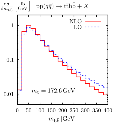
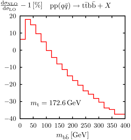
Figure 7: Distribution in the invariant mass $m_{{\mathrm{b}}{\mathrm{\bar{b}}}}$ of the bottom–antibottom pair (left) and corresponding relative NLO corrections (right) for $\mu_{\mathrm{R}}=\mu_{\mathrm{F}}=\mu_{0}=m_{\mathrm{t}}$.

The differential cross section drops strongly with increasing $m_{{\mathrm{b}}\bar{\mathrm{b}}}$, while the relative NLO corrections become large and negative. The increase of the corrections with $m_{{\mathrm{b}}\bar{\mathrm{b}}}$ is larger than the one seen in Figure 6 since the scales are fixed to $m_{\mathrm{t}}$ and not related to $m_{{\mathrm{b}}\bar{\mathrm{b}}}$. In this paper we do not investigate in how far shape distortions induced by the corrections could be absorbed into the LO upon using phase-space-dependent scales; we postpone this issue until the full NLO corrections including ${\mathrm{g}}{\mathrm{g}}$ fusion are available. The drop of the distribution for small $m_{{\mathrm{b}}\bar{\mathrm{b}}}$ is due to the fact that the jet algorithm provides an effective cut on this variable.

The distribution in the transverse momentum $p_{{\mathrm{T}},{\mathrm{b}}{\mathrm{\bar{b}}}}$ of the bottom–antibottom pair shown in Figure 8 looks very similar.

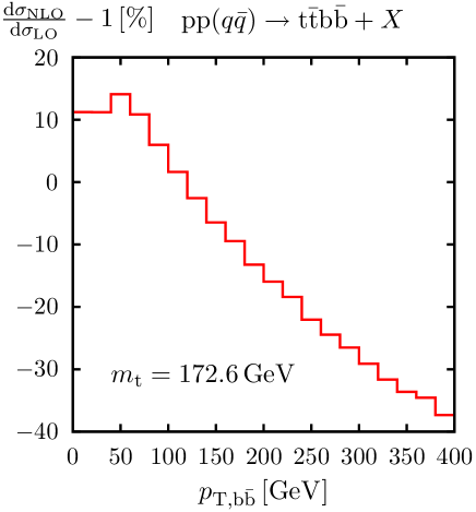
Figure 8: Distribution in the transverse momentum $p_{{\mathrm{T}},{\mathrm{b}}{\mathrm{\bar{b}}}}$ of the bottom–antibottom pair (left) and corresponding relative corrections (right) for $\mu_{\mathrm{R}}=\mu_{\mathrm{F}}=\mu_{0}=m_{\mathrm{t}}$.

Again, for our scale choice, the NLO corrections reduce the cross section for large values of $p_{{\mathrm{T}},{\mathrm{b}}{\mathrm{\bar{b}}}}$.

Finally, we depict the distribution in the rapidity $y_{{\mathrm{b}}{\mathrm{\bar{b}}}}$ of the bottom–antibottom pair in Figure 9.

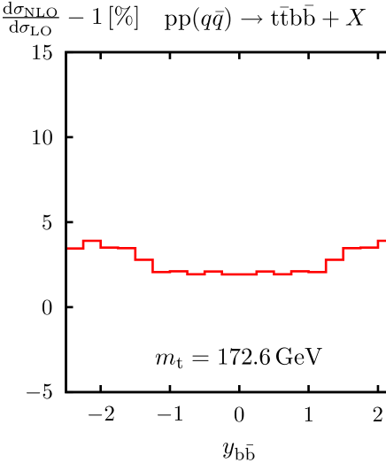
Figure 9: Distribution in the rapidity $y_{{\mathrm{b}}{\mathrm{\bar{b}}}}$ of the bottom–antibottom pair (left) and corresponding relative corrections (right) for $\mu_{\mathrm{R}}=\mu_{\mathrm{F}}=\mu_{0}=m_{\mathrm{t}}$.

In this case, the NLO corrections are rather flat at the level of 2.5% with a slight increase in the backward and forward directions.

4 Conclusions

Predictions for the background process ${\mathrm{p}}{\mathrm{p}}\to{\mathrm{t}}\bar{\mathrm{t}}{\mathrm{b}}\bar{\mathrm{b}}+X$ in NLO QCD are indispensable for a thorough analysis of ${\mathrm{t}}\bar{\mathrm{t}}{\mathrm{H}}$ production at the LHC.

In this paper we have made the first step towards the full NLO calculation upon evaluating the contribution from quark–antiquark annihilation. We made use of the Feynman-diagrammatic approach augmented by recently developed reduction techniques for one-loop tensor integrals. We have devoted an appendix to the general issue of rational terms resulting from ultraviolet or infrared (soft or collinear) singularities within dimensional regularization. In particular, we have shown that rational terms of infrared origin cancel in truncated one-loop diagrams for arbitrary processes in the Feynman gauge and thus result only from wave-function renormalization. Based on this observation we have formulated a general recipe for the determination of rational terms in one-loop amplitudes.

Our calculation demonstrates that the Feynman-diagrammatic approach can be successfully applied in the context of six-particle processes at the LHC, providing excellent numerical stability and high speed. The CPU time needed to evaluate the full virtual corrections with a single processor is of the order of $10^{-2}$ seconds per phase-space point. Based on these encouraging results, we expect to be able to extend this calculation to the technically more challenging gluon-fusion channel.

Appendix

Appendix A Rational terms in one-loop amplitudes

In this appendix we elaborate on the issue of so-called rational terms that occur within dimensional regularization when algebraic factors depending on the space–time dimensionality $D$ multiply loop integrals that contain UV or IR (soft and/or collinear) singularities, which give rise to poles in $D-4$. The calculation of rational terms is of particular importance for so-called unitarity or generalized-unitarity methods (see Refs. [10, 11, 12, 13] and references therein). In this context, these terms are typically obtained by recursion relations [59, 60, 61] or by exploiting the full $D$-dimensional dependence of the tree amplitudes [62, 12, 63]. Explicit recipes to derive rational terms in the context of specific methods, which make use of loop integrals in shifted space–time dimensions or employ a numerical reduction at the integrand level, can be found in Refs. [64, 65]. Here we discuss rational terms in the framework of one-loop calculations that employ an arbitrary set of tensor (and scalar) loop integrals in $D=4-2\epsilon$ dimensions and derive general properties that are independent of the explicit algorithm used for tensor reduction.

Specifically we investigate rational terms resulting from unrenormalized truncated loop amplitudes and do not consider external self-energy corrections (wave-function renormalization constants). Since the latter enter via derivatives, our arguments cannot be applied, but these contributions are easily calculated once and for all. We classify the different situations in which rational terms arise and describe simple procedures and results for their actual calculation. In particular, we demonstrate that—for any scattering amplitude involving quarks and gluons—the rational terms originating from IR poles cancel within individual Feynman diagrams. This important property implies that, after separating the rational terms of UV type, the coefficients of all IR-divergent tensor $N$-point integrals can be evaluated in four dimensions. In practice the wave-function renormalization constants represent the only source of rational terms of IR origin. This greatly simplifies the algebraic manipulation of IR-divergent scattering amplitudes.

A.1 Classification of rational terms

Algebraic factors containing the dimensionality $D$ result from two different sources in one-loop amplitudes:

1. “Trace-like” contractions among metric tensors or with Dirac structures lead to expressions such as $g^{\mu\nu}g_{\nu\mu}=D$, $\gamma^{\mu}\mathchoice{\hbox to0.0pt{\hss$\displaystyle/$\hss\kern-5.28589pt}\hbox{$\displaystyle a$}}{\hbox to0.0pt{\hss$\textstyle/$\hss\kern-5.28589pt}\hbox{$\textstyle a$}}{\hbox to0.0pt{\hss$\scriptstyle/$\hss\kern-3.70012pt}\hbox{$\scriptstyle a$}}{\hbox to0.0pt{\hss$\scriptscriptstyle/$\hss\kern-2.64294pt}\hbox{$\scriptscriptstyle a$}}\gamma^{\nu}g_{\mu\nu}=\gamma^{\mu}\mathchoice{\hbox to0.0pt{\hss$\displaystyle/$\hss\kern-5.28589pt}\hbox{$\displaystyle a$}}{\hbox to0.0pt{\hss$\textstyle/$\hss\kern-5.28589pt}\hbox{$\textstyle a$}}{\hbox to0.0pt{\hss$\scriptstyle/$\hss\kern-3.70012pt}\hbox{$\scriptstyle a$}}{\hbox to0.0pt{\hss$\scriptscriptstyle/$\hss\kern-2.64294pt}\hbox{$\scriptscriptstyle a$}}\gamma_{\mu}=(2-D)\mathchoice{\hbox to0.0pt{\hss$\displaystyle/$\hss\kern-5.28589pt}\hbox{$\displaystyle a$}}{\hbox to0.0pt{\hss$\textstyle/$\hss\kern-5.28589pt}\hbox{$\textstyle a$}}{\hbox to0.0pt{\hss$\scriptstyle/$\hss\kern-3.70012pt}\hbox{$\scriptstyle a$}}{\hbox to0.0pt{\hss$\scriptscriptstyle/$\hss\kern-2.64294pt}\hbox{$\scriptscriptstyle a$}}$, etc.

2. In the reduction of tensor one-loop integrals to standard scalar integrals (such as the usual Passarino–Veltman reduction [35]) the tensor coefficients are eventually obtained as linear combinations of the scalar integrals which form a basis of functions. In such linear combinations, the tensor coefficients containing metric tensors in their corresponding covariants receive prefactors with a dependence on $D$.

Thus, we can distinguish four different types of rational terms, classified according to type 1 or 2 being of UV or IR origin.

We employ the notation of Ref. [5], where the covariant coefficients of $N$-point integrals with rank $R$ are denoted as $T^{N}_{i_{1}\dots i_{R}}$. It is convenient to treat the UV- and IR-divergent parts of tensor integrals separately. To this end, we write

$$T^{N}_{i_{1}\dots i_{R}}=\hat{T}^{N}_{i_{1}\dots i_{R}}+\frac{R^{N}_{i_{1}\dots i_{R}}}{\epsilon_{\mathrm{UV}}},$$ (A.1)

where $R^{N}_{i_{1}\dots i_{R}}$ represents the (IR-finite) residue of the UV pole of $T^{N}_{i_{1}\dots i_{R}}$, and $\hat{T}^{N}_{i_{1}\dots i_{R}}$ is free from UV divergences but can contain single and double poles in $\epsilon_{\mathrm{IR}}$ resulting from soft or collinear divergences. The only IR-divergent 2-point functions are those without a scale. These represent a special case since they vanish as a result of cancellations between IR and UV poles, i.e. they are formally proportional to $(1/\epsilon_{\mathrm{UV}}-1/\epsilon_{\mathrm{IR}})$. In order to separate these UV and IR poles, we isolate the UV divergences by writing, in the notation of Ref. [5],

$$B_{\underbrace{\scriptstyle 0\dots 0}_{m}\underbrace{\scriptstyle 1\dots 1}_{n}}(0,0,0)=\hat{B}_{\underbrace{\scriptstyle 0\dots 0}_{m}\underbrace{\scriptstyle 1\dots 1}_{n}}(0,0,0)+\frac{(-1)^{n}}{n+1}\frac{\delta_{m0}}{\epsilon_{\mathrm{UV}}}.$$ (A.2)

The UV-subtracted part is IR divergent,

$$\hat{B}_{\underbrace{\scriptstyle 0\dots 0}_{m}\underbrace{\scriptstyle 1\dots 1}_{n}}(0,0,0)=-\frac{(-1)^{n}}{n+1}\frac{\delta_{m0}}{\epsilon_{\mathrm{IR}}},$$ (A.3)

and exactly cancels against the UV pole. However, we do no set scaleless 2-point integrals to zero and treat the rational terms resulting from $1/\epsilon_{\mathrm{UV}}$ and $\hat{B}_{\dots}(0,0,0)$ separately. Since scaleless 2-point functions require light-like momentum transfer ($p^{2}=0$), such integrals only occur in external self-energy corrections, i.e. in wave-function renormalization constants, and in the reduction of higher-point functions ($N>2$). In the latter case, as we will show below, the rational terms of IR origin cancel out.

A.2 Rational terms of UV origin

The residues $R^{N}_{i_{1}\dots i_{R}}$ of the UV poles of general one-loop tensor integrals are simple polynomials of the external momenta and their explicit form is well known (see, e.g., App. C of Ref. [4] and App. A of Ref. [5]). In particular, in contrast to IR divergences, the UV poles do not depend on kinematical properties of the amplitude such as on-shell relations of momenta. This renders rational terms of UV origin very simple: Terms of type 2 can be directly included in the tensor reduction in a generic way, as e.g. done in Refs. [4, 5, 35, 53], and terms of type 1 can be extracted during the algebraic reduction of each Feynman diagram by means of a trivial expansion,

$$f(D)T^{N}_{i_{1}\dots i_{R}}=f(D)\hat{T}^{N}_{i_{1}\dots i_{R}}+\left[\frac{f(4)}{\epsilon_{\mathrm{UV}}}-2f^{\prime}(4)\right]{R^{N}_{i_{1}\dots i_{R}}}.$$ (A.4)

In the following we discuss the remaining rational terms that result from $f(D)\hat{T}^{N}_{i_{1}\dots i_{R}}$ when $\hat{T}^{N}_{i_{1}\dots i_{R}}$ contains poles of IR origin.

A.3 Rational terms of IR origin

IR divergences of one-loop integrals are more complicated than UV singularities, since they depend on specific kinematical properties of amplitudes. According to Kinoshita [66] they can be classified into soft and collinear singularities as indicated in Figure 10:

         

Figure 10: Kinematical configurations for soft (left) and collinear (right) IR singularities in one-loop diagrams.

• A soft singularity arises if a massless particle is exchanged between two on-shell particles (see l.h.s. of Figure 10). The singularity is logarithmic and originates from the region in momentum space where the momentum transfer of the massless propagator tends to zero.

• A collinear singularity arises if an external line with a light-like momentum (e.g. a massless external on-shell particle) is attached to two massless propagators (see r.h.s. of Figure 10). The singularity is also logarithmic and originates from the region in momentum space where the loop momentum of the two massless propagators becomes collinear to the momentum $p$ of the external particle.

We first consider rational terms of IR origin that can result from the reduction of tensor integrals (type 2). As can, for instance, be seen from the results of Ref. [5], only tensor coefficients $T^{N}_{00\dots}$ whose covariants involve the metric tensor can get $D$-dependent prefactors in reduction identities and could, thus, lead to rational terms of type 2. In Section 5.8 of Ref. [5] it was, however, shown that these tensor coefficients are IR finite. Thus, no type 2 rational terms of IR origin can result at all.

Moreover, reparametrizations of tensor integrals resulting from shifts of the loop momentum and permutations of the propagators do not give rise to $D$-dependent factors or relations between (IR-finite) tensor coefficients of type $T^{N}_{00\dots}$ and IR-singular integrals. Therefore, in order to demonstrate that a certain diagram is free from IR rational terms it is sufficient to find for each soft- or collinear-singular region a specific representation that is manifestly free from IR rational terms of type 1, i.e. to find an expression in which the corresponding IR-divergent part is expressed as a linear combination of IR-divergent tensor (or scalar) integrals with coefficients that are independent of $D$. In explicit calculations, this can be achieved by means of an algebraic reduction that implements all possible relations between the IR-divergent parts of tensor integrals. This task is non-trivial since the standard scalar integrals do not provide a unique representation of IR divergences. For instance, IR-finite parts of a diagram can be expressed as linear combinations of IR-divergent 4-point and 3-point scalar integrals. More generally, IR-singular $N$-point tensor integrals can be expressed in terms of IR-divergent 3- and 2-point scalar integrals plus IR-finite terms. This reduction of IR singularities is explicitly implemented in the algorithm presented in Ref. [37] and can be summarized by the following formula (see Eq. (3.14) in Ref. [37]) which relates the IR-divergent part of $N$-point tensor integrals to 3-point tensor integrals associated with the IR-divergent triangle subdiagrams,

$$T^{N}_{\mu_{1}\dots\mu_{R}}(p_{0},\dots,p_{N-1},m_{0},\dots,m_{N-1})$$ (A.5)

$$= \sum_{n=0}^{N-1}\sum_{k=0\atop k\neq n,n+1}^{N-1}A_{nk}C_{\mu_{1}\dots\mu_{R}}(p_{n},p_{n+1},p_{k},m_{n},m_{n+1},m_{k})+\mbox{IR-finite part}.$$

The coefficients $A_{nk}$ are independent of $D$ since all relations between IR-divergent tensor integrals are free from $D$-dimensional coefficients. For the explicit form of $A_{nk}$ and details of the notation we refer to Ref. [37]. In practice, using (A.5) and performing a subsequent reduction to scalar integrals, one can construct a unique representation of IR divergences in terms of 3- and 2-point scalar functions. The 3-point functions on the right-hand side of (A.5) can be subtracted from the complete tensor integral leading to an IR-finite expression which can be evaluated in 4 dimensions. Thus, only the re-added 3-point functions (A.5) have to be manipulated in $D$ dimensions.

Using this approach, we have observed in explicit calculations for ${\mathrm{p}}{\mathrm{p}}\to{\mathrm{t}}\bar{\mathrm{t}}{\mathrm{H}}$ [27], ${\mathrm{p}}{\mathrm{p}}\to{\mathrm{t}}\bar{\mathrm{t}}+\mathrm{jet}$ [28], and ${\mathrm{p}}{\mathrm{p}}\to{\mathrm{W}}{\mathrm{W}}+\mathrm{jet}$ [16] that—after complete reduction of the IR divergences—the coefficients of the IR-singular $C_{0}$ and $B_{0}$ functions are independent of $D$, i.e. that rational terms of IR type cancel completely. This indicates, a posteriori, that the terms $f(D)\hat{T}^{N}_{i_{1}\dots i_{R}}$ in (A.4) can be replaced by $f(4)\hat{T}^{N}_{i_{1}\dots i_{R}}$ from the beginning in the calculation. In the following we demonstrate that, in the Feynman gauge, the cancellation of IR rational terms is a general property of scattering amplitudes involving an arbitrary number of external quarks and gluons.

To this end, we inspect the integrand of a general one-loop IR-divergent diagram in momentum space and, in the spirit of Ref. [37], we separate the IR singularities associated with different soft and collinear regions and relate them to triangle subdiagrams. Using on-shell relations we show that, in the soft and collinear regions, the integrands can be cast into a form that is free from “trace-like” contractions, which potentially produce $D$-dependent factors. In this way we obtain a generic representation of the IR singularities that is manifestly free from rational terms of IR type.

The considerations presented in the following are not new. A similar approach is used, for instance, in Ref. [67], where IR and UV singularities are subtracted at the diagrammatic level and isolated in simple process-independent terms in order to obtain numerically integrable expressions. Using similar techniques, here we consider soft and collinear contributions from the perspective of an analytic calculation in terms of divergent one-loop tensor and scalar integrals and discuss the rational terms associated with IR divergences.

(i) Soft singularities:

Figure 11 shows all potentially soft-divergent subdiagrams containing quarks, gluons, or Faddeev–Popov ghosts.

Figure 11: Subdiagrams containing soft-singular integrals, with solid lines indicating quarks, epicycles gluons, and dotted lines ghosts.

Since the soft singularity is related to zero-momentum transfer on the internal line linking the two external particles, it is convenient to identify the integration momentum $q$ of the loop integral with the momentum on this line. Since the soft singularity is logarithmic, all contributions of $q$ in the numerator of the integral are IR finite. In other words, being only after the IR-divergent part we can set $q$ to zero in the numerator and in propagators that do not belong to the soft-singular triangle subdiagram. This procedure immediately kills the three subintegrals (b)–(d) with a quark on the $q$ line because of the factor $\textstyle/$$\textstyle q$ in the (massless) quark propagator. Diagram (g) with a ghost coupling to external gluons does not contribute either, because the integrand receives factors (depending on the gauge) of $q\varepsilon_{a}\to 0$ or $p_{a}\varepsilon_{a}=0$ from the coupling of the ghost to the on-shell gluon with momentum $p_{a}$ and polarization vector $\varepsilon_{a}$. The amplitude ${\cal{M}}_{(8\mathrm{a})}$ of diagram (a), of course, involves a soft singularity, but without any $D$ dependence, as can be seen in the following example where we consider an outgoing quark–antiquark pair,

$${\cal{M}}_{(8\mathrm{a})} = \int{\mathrm{d}}^{D}q\;\frac{g^{\mu\nu}}{q^{2}}\,\bar{u}_{a}(p_{a})\,\gamma_{\mu}\,\frac{\mathchoice{\hbox to0.0pt{\hss$\displaystyle/$\hss\kern-4.8229pt}\hbox{$\displaystyle q$}}{\hbox to0.0pt{\hss$\textstyle/$\hss\kern-4.8229pt}\hbox{$\textstyle q$}}{\hbox to0.0pt{\hss$\scriptstyle/$\hss\kern-3.37604pt}\hbox{$\scriptstyle q$}}{\hbox to0.0pt{\hss$\scriptscriptstyle/$\hss\kern-2.41144pt}\hbox{$\scriptscriptstyle q$}}+\mathchoice{\hbox to0.0pt{\hss$\displaystyle/$\hss\kern-5.03125pt}\hbox{$\displaystyle p$}}{\hbox to0.0pt{\hss$\textstyle/$\hss\kern-5.03125pt}\hbox{$\textstyle p$}}{\hbox to0.0pt{\hss$\scriptstyle/$\hss\kern-3.52188pt}\hbox{$\scriptstyle p$}}{\hbox to0.0pt{\hss$\scriptscriptstyle/$\hss\kern-2.51563pt}\hbox{$\scriptscriptstyle p$}}_{a}+m_{a}}{(q+p_{a})^{2}-m_{a}^{2}}\,\Gamma(q)\,\frac{\mathchoice{\hbox to0.0pt{\hss$\displaystyle/$\hss\kern-4.8229pt}\hbox{$\displaystyle q$}}{\hbox to0.0pt{\hss$\textstyle/$\hss\kern-4.8229pt}\hbox{$\textstyle q$}}{\hbox to0.0pt{\hss$\scriptstyle/$\hss\kern-3.37604pt}\hbox{$\scriptstyle q$}}{\hbox to0.0pt{\hss$\scriptscriptstyle/$\hss\kern-2.41144pt}\hbox{$\scriptscriptstyle q$}}-\mathchoice{\hbox to0.0pt{\hss$\displaystyle/$\hss\kern-5.03125pt}\hbox{$\displaystyle p$}}{\hbox to0.0pt{\hss$\textstyle/$\hss\kern-5.03125pt}\hbox{$\textstyle p$}}{\hbox to0.0pt{\hss$\scriptstyle/$\hss\kern-3.52188pt}\hbox{$\scriptstyle p$}}{\hbox to0.0pt{\hss$\scriptscriptstyle/$\hss\kern-2.51563pt}\hbox{$\scriptscriptstyle p$}}_{b}+m_{b}}{(q-p_{b})^{2}-m_{b}^{2}}\,\gamma_{\nu}\,v_{b}(p_{b})$$ (A.6)

$$= \int{\mathrm{d}}^{D}q\;\frac{g^{\mu\nu}}{q^{2}}\,\bar{u}_{a}(p_{a})\,\gamma_{\mu}\,\frac{\mathchoice{\hbox to0.0pt{\hss$\displaystyle/$\hss\kern-5.03125pt}\hbox{$\displaystyle p$}}{\hbox to0.0pt{\hss$\textstyle/$\hss\kern-5.03125pt}\hbox{$\textstyle p$}}{\hbox to0.0pt{\hss$\scriptstyle/$\hss\kern-3.52188pt}\hbox{$\scriptstyle p$}}{\hbox to0.0pt{\hss$\scriptscriptstyle/$\hss\kern-2.51563pt}\hbox{$\scriptscriptstyle p$}}_{a}+m_{a}}{(q+p_{a})^{2}-m_{a}^{2}}\,\Gamma(0)\,\frac{-\mathchoice{\hbox to0.0pt{\hss$\displaystyle/$\hss\kern-5.03125pt}\hbox{$\displaystyle p$}}{\hbox to0.0pt{\hss$\textstyle/$\hss\kern-5.03125pt}\hbox{$\textstyle p$}}{\hbox to0.0pt{\hss$\scriptstyle/$\hss\kern-3.52188pt}\hbox{$\scriptstyle p$}}{\hbox to0.0pt{\hss$\scriptscriptstyle/$\hss\kern-2.51563pt}\hbox{$\scriptscriptstyle p$}}_{b}+m_{b}}{(q-p_{b})^{2}-m_{b}^{2}}\,\gamma_{\nu}\,v_{b}(p_{b})+\dots$$

$$= -4(p_{a}p_{b})\int{\mathrm{d}}^{D}q\;\frac{\bar{u}_{a}(p_{a})\,\Gamma(0)\,v_{b}(p_{b})}{q^{2}[(q+p_{a})^{2}-m_{a}^{2}][(q-p_{b})^{2}-m_{b}^{2}]}+\dots\,.$$

The Dirac structure $\Gamma(q)$ contains the remaining part of the diagram and the ellipses stand for terms that are not singular if the gluon becomes soft. For the last equality the Dirac equation was used twice. The soft singularity, which is just contained in the scalar 3-point function, does not receive $D$-dependent factors and, thus, does not deliver rational terms, because $\Gamma(0)$ is a tree-like structure and does not contain a trace-like contraction that would lead to factors of $D$. Such factors, e.g., arise in terms like $\gamma^{\mu}\Gamma(0)\gamma_{\mu}$, which are absent in the soft-singular part. The same reasoning applies also to all other possible fermion-number flows in diagram (a). The remaining two diagrams (e) and (f) of Figure 10 can be analysed in the same way, leading to the same conclusion that no $D$-dependent factors multiply soft-singular integrals. For brevity we show this only for diagram (f) explicitly,

$${\cal{M}}_{(8\mathrm{f})} = \int{\mathrm{d}}^{D}q\;\frac{g^{\lambda\sigma}}{q^{2}}\,\varepsilon^{\mu*}_{a}\,\frac{g_{\mu\nu}(q+2p_{a})_{\lambda}-g_{\nu\lambda}(2q+p_{a})_{\mu}+g_{\lambda\mu}(q-p_{a})_{\nu}}{(q+p_{a})^{2}}\,\Gamma^{\nu\tau}(q)$$ (A.7)

$${}\qquad\times\varepsilon^{\rho*}_{b}\,\frac{g_{\rho\tau}(-q+2p_{b})_{\sigma}+g_{\tau\sigma}(2q-p_{b})_{\rho}-g_{\sigma\rho}(q+p_{b})_{\tau}}{(q-p_{b})^{2}}$$

$$= \int{\mathrm{d}}^{D}q\;\frac{g^{\lambda\sigma}}{q^{2}}\,\varepsilon^{\mu*}_{a}\frac{2g_{\mu\nu}p_{a,\lambda}-g_{\nu\lambda}p_{a,\mu}-g_{\lambda\mu}p_{a,\nu}}{(q+p_{a})^{2}}\,\Gamma^{\nu\tau}(0)$$

$${}\qquad\times\varepsilon^{\rho*}_{b}\frac{2g_{\rho\tau}p_{b,\sigma}-g_{\tau\sigma}p_{b,\rho}-g_{\sigma\rho}p_{b,\tau}}{(q-p_{b})^{2}}+\dots$$

$$= \int{\mathrm{d}}^{D}q\;\frac{[4(p_{a}p_{b})\varepsilon^{*}_{a,\nu}\varepsilon^{*}_{b,\tau}-2(\varepsilon^{*}_{a}p_{b})p_{a,\nu}\varepsilon^{*}_{b,\tau}-2(p_{a}\varepsilon^{*}_{b})\varepsilon^{*}_{a,\nu}p_{b,\tau}+(\varepsilon^{*}_{a}\varepsilon^{*}_{b})p_{a,\nu}p_{b,\tau}]\Gamma^{\nu\tau}(0)}{q^{2}(q+p_{a})^{2}(q-p_{b})^{2}}$$

$$\qquad{}+\;\dots\,,$$

where we assume the external on-shell gluons to be outgoing. The last line of this result cannot contain explicit factors of $D$, since those would require a trace-like contraction ${\Gamma^{\nu}}_{\nu}(0)$; instead $\Gamma$ is only contracted with momenta $p_{a,b}$ and polarization vectors $\varepsilon^{*}_{a,b}$. Formally the contraction ${\Gamma^{\nu}}_{\nu}(0)$ occurs, but with a proportionality to $(p_{a}\varepsilon^{*}_{a})(p_{b}\varepsilon^{*}_{b})$ which vanishes owing to the on-shell condition of the gluons.

It is well known that the soft singularities are ruled by the eikonal current, with the result that divergences connected to soft-particle exchange between $a$ and $b$ are proportional to $(p_{a}p_{b})$. For ${\cal{M}}_{(8\mathrm{a})}$ this factor is already explicit in (A.6), for ${\cal{M}}_{(8\mathrm{f})}$ in (A.7) this fact becomes obvious after making use of the Ward identities $p_{a,\nu}\varepsilon^{*}_{b,\tau}\Gamma^{\nu\tau}(0)=\varepsilon^{*}_{a,\nu}p_{b,\tau}\Gamma^{\nu\tau}(0)=p_{a,\nu}p_{b,\tau}\Gamma^{\nu\tau}(0)=0$, which are valid if all other external particles are on shell and all diagrams contributing to $\Gamma$ are summed over.

(ii) Collinear singularities:

Figure 12 shows all potentially collinear-divergent subdiagrams containing (massless) quarks, gluons, or Faddeev–Popov ghosts.

Figure 12: Subdiagrams containing collinear-singular integrals, with solid lines indicating quarks, epicycles gluons, and dotted lines ghosts.

We identify the integration momentum $q$ with the momentum of one of the two propagators attached to the external light-like line, which carries the momentum $p$ ($p^{2}=0$). The collinear singularity stems from the region in $q$ space where $q$ is collinear to $p$, i.e. $q^{\mu}=x(q)p^{\mu}$ with some scalar function $x(q)$. Since the singularity is only logarithmic, we do not change the singularity if we replace $q^{\mu}$ by $x(q)p^{\mu}$ in the numerator of the amplitude. The on-shell conditions (Dirac equation for quarks and transversality condition for gluons) then imply that the collinear-singular parts of diagrams (a)–(d) in Figure 12 do not receive $D$-dependent factors:

$${\cal{M}}_{(9\mathrm{a})} = \int{\mathrm{d}}^{D}q\;\frac{1}{q^{2}}\,\bar{u}(p)\,\gamma_{\mu}\,\frac{\mathchoice{\hbox to0.0pt{\hss$\displaystyle/$\hss\kern-4.8229pt}\hbox{$\displaystyle q$}}{\hbox to0.0pt{\hss$\textstyle/$\hss\kern-4.8229pt}\hbox{$\textstyle q$}}{\hbox to0.0pt{\hss$\scriptstyle/$\hss\kern-3.37604pt}\hbox{$\scriptstyle q$}}{\hbox to0.0pt{\hss$\scriptscriptstyle/$\hss\kern-2.41144pt}\hbox{$\scriptscriptstyle q$}}+\mathchoice{\hbox to0.0pt{\hss$\displaystyle/$\hss\kern-5.03125pt}\hbox{$\displaystyle p$}}{\hbox to0.0pt{\hss$\textstyle/$\hss\kern-5.03125pt}\hbox{$\textstyle p$}}{\hbox to0.0pt{\hss$\scriptstyle/$\hss\kern-3.52188pt}\hbox{$\scriptstyle p$}}{\hbox to0.0pt{\hss$\scriptscriptstyle/$\hss\kern-2.51563pt}\hbox{$\scriptscriptstyle p$}}}{(q+p)^{2}}\,\Gamma^{\mu}(q)$$ (A.8)

$$= \int{\mathrm{d}}^{D}q\;\frac{1}{q^{2}}\,\bar{u}(p)\,\gamma_{\mu}\,\frac{[1+x(q)]\mathchoice{\hbox to0.0pt{\hss$\displaystyle/$\hss\kern-5.03125pt}\hbox{$\displaystyle p$}}{\hbox to0.0pt{\hss$\textstyle/$\hss\kern-5.03125pt}\hbox{$\textstyle p$}}{\hbox to0.0pt{\hss$\scriptstyle/$\hss\kern-3.52188pt}\hbox{$\scriptstyle p$}}{\hbox to0.0pt{\hss$\scriptscriptstyle/$\hss\kern-2.51563pt}\hbox{$\scriptscriptstyle p$}}}{(q+p)^{2}}\,\Gamma^{\mu}(x(q)p)+\dots$$

$$= \int{\mathrm{d}}^{D}q\;\frac{2[1+x(q)]\bar{u}(p)p_{\mu}\Gamma^{\mu}(x(q)p)}{q^{2}(q+p)^{2}}\,+\dots\,,$$

$${\cal{M}}_{(9\mathrm{b})} = \int{\mathrm{d}}^{D}q\;\frac{1}{q^{2}(q+p)^{2}}\,{\left[\mathchoice{\hbox to0.0pt{\hss$\displaystyle/$\hss\kern-4.8229pt}\hbox{$\displaystyle q$}}{\hbox to0.0pt{\hss$\textstyle/$\hss\kern-4.8229pt}\hbox{$\textstyle q$}}{\hbox to0.0pt{\hss$\scriptstyle/$\hss\kern-3.37604pt}\hbox{$\scriptstyle q$}}{\hbox to0.0pt{\hss$\scriptscriptstyle/$\hss\kern-2.41144pt}\hbox{$\scriptscriptstyle q$}}\,\mathchoice{\hbox to0.0pt{\hss$\displaystyle/$\hss\kern-4.66318pt}\hbox{$\displaystyle\varepsilon$}}{\hbox to0.0pt{\hss$\textstyle/$\hss\kern-4.66318pt}\hbox{$\textstyle\varepsilon$}}{\hbox to0.0pt{\hss$\scriptstyle/$\hss\kern-3.26422pt}\hbox{$\scriptstyle\varepsilon$}}{\hbox to0.0pt{\hss$\scriptscriptstyle/$\hss\kern-2.33159pt}\hbox{$\scriptscriptstyle\varepsilon$}}^{*}\,(\mathchoice{\hbox to0.0pt{\hss$\displaystyle/$\hss\kern-4.8229pt}\hbox{$\displaystyle q$}}{\hbox to0.0pt{\hss$\textstyle/$\hss\kern-4.8229pt}\hbox{$\textstyle q$}}{\hbox to0.0pt{\hss$\scriptstyle/$\hss\kern-3.37604pt}\hbox{$\scriptstyle q$}}{\hbox to0.0pt{\hss$\scriptscriptstyle/$\hss\kern-2.41144pt}\hbox{$\scriptscriptstyle q$}}+\mathchoice{\hbox to0.0pt{\hss$\displaystyle/$\hss\kern-5.03125pt}\hbox{$\displaystyle p$}}{\hbox to0.0pt{\hss$\textstyle/$\hss\kern-5.03125pt}\hbox{$\textstyle p$}}{\hbox to0.0pt{\hss$\scriptstyle/$\hss\kern-3.52188pt}\hbox{$\scriptstyle p$}}{\hbox to0.0pt{\hss$\scriptscriptstyle/$\hss\kern-2.51563pt}\hbox{$\scriptscriptstyle p$}})\right]_{\alpha\beta}}\,\Gamma_{\alpha\beta}(q)$$ (A.9)

$$= \int{\mathrm{d}}^{D}q\;\frac{x(q)[1+x(q)]}{q^{2}(q+p)^{2}}\,{\left[\mathchoice{\hbox to0.0pt{\hss$\displaystyle/$\hss\kern-5.03125pt}\hbox{$\displaystyle p$}}{\hbox to0.0pt{\hss$\textstyle/$\hss\kern-5.03125pt}\hbox{$\textstyle p$}}{\hbox to0.0pt{\hss$\scriptstyle/$\hss\kern-3.52188pt}\hbox{$\scriptstyle p$}}{\hbox to0.0pt{\hss$\scriptscriptstyle/$\hss\kern-2.51563pt}\hbox{$\scriptscriptstyle p$}}\,\mathchoice{\hbox to0.0pt{\hss$\displaystyle/$\hss\kern-4.66318pt}\hbox{$\displaystyle\varepsilon$}}{\hbox to0.0pt{\hss$\textstyle/$\hss\kern-4.66318pt}\hbox{$\textstyle\varepsilon$}}{\hbox to0.0pt{\hss$\scriptstyle/$\hss\kern-3.26422pt}\hbox{$\scriptstyle\varepsilon$}}{\hbox to0.0pt{\hss$\scriptscriptstyle/$\hss\kern-2.33159pt}\hbox{$\scriptscriptstyle\varepsilon$}}^{*}\,\mathchoice{\hbox to0.0pt{\hss$\displaystyle/$\hss\kern-5.03125pt}\hbox{$\displaystyle p$}}{\hbox to0.0pt{\hss$\textstyle/$\hss\kern-5.03125pt}\hbox{$\textstyle p$}}{\hbox to0.0pt{\hss$\scriptstyle/$\hss\kern-3.52188pt}\hbox{$\scriptstyle p$}}{\hbox to0.0pt{\hss$\scriptscriptstyle/$\hss\kern-2.51563pt}\hbox{$\scriptscriptstyle p$}}\right]_{\alpha\beta}}\,\Gamma_{\alpha\beta}(x(q)p)+\dots$$

$$= \int{\mathrm{d}}^{D}q\;\frac{x(q)[1+x(q)]}{q^{2}(q+p)^{2}}\,{2(\varepsilon^{*}p)\,\left[\mathchoice{\hbox to0.0pt{\hss$\displaystyle/$\hss\kern-5.03125pt}\hbox{$\displaystyle p$}}{\hbox to0.0pt{\hss$\textstyle/$\hss\kern-5.03125pt}\hbox{$\textstyle p$}}{\hbox to0.0pt{\hss$\scriptstyle/$\hss\kern-3.52188pt}\hbox{$\scriptstyle p$}}{\hbox to0.0pt{\hss$\scriptscriptstyle/$\hss\kern-2.51563pt}\hbox{$\scriptscriptstyle p$}}\right]_{\alpha\beta}}\,\Gamma_{\alpha\beta}(x(q)p)+\dots$$

$$= 0+\dots\,,$$

$${\cal{M}}_{(9\mathrm{c})} = \int{\mathrm{d}}^{D}q\;\varepsilon^{\mu*}\,\frac{g_{\mu\nu}(q+2p)_{\lambda}-g_{\nu\lambda}(2q+p)_{\mu}+g_{\lambda\mu}(q-p)_{\nu}}{q^{2}(q+p)^{2}}\,\Gamma^{\nu\lambda}(q)$$ (A.10)

$$= \int{\mathrm{d}}^{D}q\;\varepsilon^{\mu*}\,\frac{g_{\mu\nu}(x(q)+2)p_{\lambda}-g_{\nu\lambda}(2x(q)+1)p_{\mu}+g_{\lambda\mu}(x(q)-1)p_{\nu}}{q^{2}(q+p)^{2}}\,\Gamma^{\nu\lambda}(x(q)p)+\dots$$

$$= \int{\mathrm{d}}^{D}q\;\frac{[(x(q)+2)\varepsilon^{*}_{\nu}p_{\lambda}+(x(q)-1)\varepsilon^{*}_{\lambda}p_{\nu}]\,\Gamma^{\nu\lambda}(x(q)p)}{q^{2}(q+p)^{2}}+\dots\,,$$

$${\cal{M}}_{(9\mathrm{d})} = \int{\mathrm{d}}^{D}q\;\varepsilon^{\mu*}\,\frac{q_{\mu}}{q^{2}(q+p)^{2}}\,\Gamma(q)$$ (A.11)

$$= \int{\mathrm{d}}^{D}q\;\varepsilon^{\mu*}\,\frac{x(q)p_{\mu}}{q^{2}(q+p)^{2}}\,\Gamma(x(q)p)$$

$$= 0+\dots\,.$$

Note that diagrams (b) and (d) do not have collinear singularities at all. The collinear divergences in diagrams (a) and (c) do not receive $D$-dependent factors since, in the collinear region, the $\Gamma$ terms do not take part in trace-like contractions like $\gamma_{\mu}\Gamma^{\mu}$ or ${\Gamma^{\nu}}_{\nu}$, and terms $q^{\tau_{1}}\dots q^{\tau_{n}}$ inside $\Gamma$ yield tensor structures $[x(q)]^{n}p^{\tau_{1}}\dots p^{\tau_{n}}$ without metric tensors. The above IR-divergent integrals are easily expressed in terms of usual 3-point functions by observing that in the collinear limit all propagators inside $\Gamma(x(q)p)$ are linear in $x(q)$ owing to $(q+p_{k})^{2}\to 2x(q)pp_{k}+p_{k}^{2}$. Thus, one can easily express the denominator of $\Gamma(x(q)p)$ as a linear combination of single propagators via partial fractioning, as done in Ref. [37].

In summary we have obtained a representation of the soft and collinear singularities of generic Feynman diagrams in terms of 3-point tensor integrals that are explicitly free from $D$-dimensional prefactors. We can, thus, conclude that rational terms of IR origin cancel in any unrenormalized scattering amplitude and can be neglected a priori in explicit calculations. This property is a consequence of the Lorentz structure of the gluon couplings and the logarithmic nature of IR singularities within the conventional Feynman gauge. However, the cancellation of IR rational terms holds also in more general gauge-fixings, as for instance the background-field Feynman gauge (see Ref. [68] and references therein), where the Lorentz structures in the gluon couplings and the poles of the propagators behave as in the Feynman gauge.

We point out that the cancellation of IR rational terms is independent of the actual reduction method employed in the calculation and is generally valid in any approach where the IR-divergent parts of loop diagrams are entirely expressed in terms of tensor (or scalar) $N$-point integrals in $4-2\epsilon$ dimensions.

A.4 A recipe for determining rational terms

Based on the above considerations we can formulate a simple algorithm for determining all rational terms of either UV or IR origin. For unrenormalized truncated one-loop diagrams, i.e. excluding counterterm diagrams and self-energy corrections to external lines, proceed as follows:

1. Separate UV and IR divergences of all tensor integrals as in (A.1), thereby keeping track of the poles of all scaleless 2-point integrals as indicated in (A.2) and (A.3).

2. Extract the rational terms of UV origin as described in (A.4) including the rational terms resulting from UV poles of scaleless 2-point integrals.

3. Ignore rational terms of IR origin upon replacing $f(D)\to f(4)$ on the right-hand side of (A.4), because the arguments of the previous section show that all rational terms resulting from $[f(D)-f(4)]\hat{T}^{N}_{i_{1}\dots i_{R}}$ in (A.4) compensate each other (even if they may arise in intermediate steps).

This recipe does not apply to wave-function renormalization constants. These can be easily calculated, and explicit results are, e.g., given in Eqs. (2.27)–(2.28) of Ref. [27].

Appendix B Four-dimensional reduction of Dirac chains to standard matrix elements

Here we outline the algebraic procedure employed to reduce Dirac structures to standard matrix elements. The reduction is based on the strategy described in Sect. 3.3 of Ref. [29], which is worked out for massless six-fermion processes, and involves additional features to treat the Dirac chains associated with massive top quarks. This method exploits a set of relations that do not give rise to denominators involving kinematical variables, thereby avoiding possible numerical instabilities in exceptional phase-space regions. Refraining from a detailed description of the entire reduction algorithm, which is quite involved, we only outline the basic principles, which can be traced back to a few simple identities.

Tree and loop diagrams give rise to a large number of Dirac structures of the type

$$\bar{v}(p_{1})\gamma^{\mu_{1}}\ldots{p/_{i_{1}}}\ldots u(p_{2})\;\bar{v}(p_{3})\gamma^{\nu_{1}}\ldots{p/_{j_{1}}}\ldots u(p_{4})\;\bar{v}(p_{5})\gamma^{\rho_{1}}\ldots{p/_{k_{1}}}\ldots u(p_{6}),$$ (B.1)

which consist of gamma matrices (or slashed momenta) that are sandwiched between the spinors $\bar{v}(p_{a})$ and $u(p_{a+1})$ of the six (anti)fermions. For convenience we consider the crossed process $\bar{q}q\bar{\mathrm{t}}{\mathrm{t}}\bar{\mathrm{b}}{\mathrm{b}}\to 0$, where all particles and their momenta are incoming. While the chains associated with massless quarks ($a=1,5$) contain only odd numbers of Dirac matrices, inside the top chain ($a=3$) also even numbers of Dirac matrices appear. The open Lorentz indices $\mu_{i},\nu_{j},\rho_{k}$ in (B.1) are always pairwise contracted via the metric tensor.

The combinations of Dirac matrices occurring inside individual chains $\bar{v}(p_{a})\dots u(p_{a+1})$ can easily be simplified by means of elementary relations:

1. Standard Dirac algebra permits to reduce $\gamma^{\mu}\dots\gamma_{\mu}$ contractions inside Dirac chains, to bring gamma matrices and $p/$ terms into a standard order through anti-commutations, and to eliminate $p/^{2}$ terms.

2. All $p/_{a}$ and $p/_{a+1}$ terms can be eliminated with the Dirac equation.

3. The $p/_{i}$ terms associated with one of the other external momenta ($i\neq a,a+1$) can be eliminated via momentum conservation.

After these simplifications, which we perform in $D$ dimensions, we are left with a still large number of Dirac structures of $\mathcal{O}(10^{3})$. To obtain a further reduction we employ additional identities which permit to shift $p/$ terms and $\gamma^{\mu}$ matrices with open indices from one chain to another, thereby permitting further simplifications of type (i)–(iii). This part of the reduction relies on four-dimensional relations and is performed after separation of all $(D-4)$-poles in dimensional regularization.

All four-dimensional identities are derived from basic relations which follow from Chisholm’s identity (see Eqs. (3.4)–(3.6) in Ref. [29]) and read

$${\gamma^{\mu}}{\gamma^{\alpha}\gamma^{\beta}}\omega_{\pm}\otimes{\gamma_{\mu}} = {\gamma^{\mu}}\omega_{\pm}\otimes\left(\gamma_{\mu}\gamma^{\beta}\gamma^{\alpha}\omega_{\pm}+\gamma^{\alpha}\gamma^{\beta}\gamma_{\mu}\omega_{\mp}\right),$$

$${\gamma^{\alpha}}{\gamma^{\mu}\gamma^{\beta}}\omega_{\pm}\otimes{\gamma_{\mu}} = {\gamma^{\mu}}\omega_{\pm}\otimes\left(\gamma^{\beta}\gamma_{\mu}\gamma^{\alpha}\omega_{\pm}+\gamma^{\alpha}\gamma_{\mu}\gamma^{\beta}\omega_{\mp}\right),$$

$${\gamma^{\alpha}}{\gamma^{\beta}\gamma^{\mu}}\omega_{\pm}\otimes{\gamma_{\mu}} = {\gamma^{\mu}}\omega_{\pm}\otimes\left(\gamma^{\beta}\gamma^{\alpha}\gamma_{\mu}\omega_{\pm}+\gamma_{\mu}\gamma^{\alpha}\gamma^{\beta}\omega_{\mp}\right),$$ (B.2)

where $\omega_{\pm}=(1\pm\gamma^{5})/2$ are the chirality projectors and the tensor products connect different Dirac chains. In order to exploit these relations we introduce chirality projectors inside every Dirac chain, $\bar{v}(p_{a})\Gamma u(p_{a+1})=\sum_{\lambda=\pm}\bar{v}(p_{a})\Gamma\omega_{\lambda}u(p_{a+1}).$ Then we can use (B) to exchange $\gamma^{\alpha}\gamma^{\beta}$-terms between chains that are connected via $\gamma^{\mu}$-contractions. A simple application of (B) is given by

$${\gamma^{\mu}}{\gamma^{\alpha}}{\gamma^{\nu}}\omega_{\pm}\otimes{\gamma_{\mu}}{\gamma^{\beta}}{\gamma_{\nu}}=4g^{\alpha\beta}{\gamma^{\mu}}\omega_{\pm}\otimes\gamma_{\mu}\omega_{\pm}+4\gamma^{\beta}\omega_{\pm}\otimes\gamma^{\alpha}\omega_{\mp},$$

$${\gamma^{\mu}}{\gamma^{\alpha}}{\gamma^{\nu}}\omega_{\pm}\otimes{\gamma_{\nu}}{\gamma^{\beta}}{\gamma_{\mu}}=4g^{\alpha\beta}{\gamma^{\mu}}\omega_{\pm}\otimes\gamma_{\mu}\omega_{\mp}+4\gamma^{\beta}\omega_{\pm}\otimes\gamma^{\alpha}\omega_{\pm}.$$ (B.3)

These identities permit to eliminate double Lorentz contractions between two Dirac chains. Alternatively we can use (B) in the opposite direction, in combination with the Dirac equation. This yields the relations

$$p/_{b}\omega_{\pm}u(p_{a})\otimes p/_{a}\omega_{\mp}u(p_{b})=(p_{a}p_{b})\gamma^{\mu}\omega_{\pm}u(p_{a})\otimes\gamma_{\mu}\omega_{\mp}u(p_{b})$$

$${}-\frac{m_{a}}{2}\gamma^{\mu}p/_{b}\omega_{\mp}u(p_{a})\otimes\gamma_{\mu}\omega_{\mp}u(p_{b})-\frac{m_{b}}{2}\gamma^{\mu}\omega_{\pm}u(p_{a})\otimes\gamma_{\mu}p/_{a}\omega_{\pm}u(p_{b})+m_{a}m_{b}\mbox{-term},$$

$$\bar{v}(p_{a})p/_{b}\omega_{\pm}\otimes\bar{v}(p_{b})p/_{a}\omega_{\mp}=(p_{a}p_{b})\bar{v}(p_{a})\gamma^{\mu}\omega_{\pm}\otimes\bar{v}(p_{b})\gamma_{\mu}\omega_{\mp}$$

$${}+\frac{m_{a}}{2}\bar{v}(p_{a})p/_{b}\gamma^{\mu}\omega_{\pm}\otimes\bar{v}(p_{b})\gamma_{\mu}\omega_{\mp}+\frac{m_{b}}{2}\bar{v}(p_{a})\gamma^{\mu}\omega_{\pm}\otimes\bar{v}(p_{b})p/_{a}\gamma_{\mu}\omega_{\mp}+m_{a}m_{b}\mbox{-term},$$

$$\bar{v}(p_{a})p/_{b}\omega_{\pm}\otimes p/_{a}\omega_{\pm}u(p_{b})=(p_{a}p_{b})\bar{v}(p_{a})\gamma^{\mu}\omega_{\pm}\otimes\gamma_{\mu}\omega_{\pm}u(p_{b})$$ (B.4)

$${}+\frac{m_{a}}{2}\bar{v}(p_{a})p/_{b}\gamma^{\mu}\omega_{\pm}\otimes\gamma_{\mu}\omega_{\pm}u(p_{b})+\frac{m_{b}}{2}\bar{v}(p_{a})\gamma^{\mu}\omega_{\pm}\otimes p/_{a}\gamma_{\mu}\omega_{\mp}u(p_{b}),$$

where the terms proportional to $m_{a}m_{b}$ vanish since the (anti)spinors associated with particles $a$ and $b$ belong to different Dirac chains and, thus, at least one of them is massless in our case. The relations (B) can be used to reduce the number of $p/_{i}$ terms in the Dirac chains.

We give two explicit examples to illustrate the four-dimensional reduction of Dirac structures that involve one massive Dirac chain:

• Example 1:
  We reduce terms involving double contractions of the type $\gamma^{\mu}\gamma^{\nu}\otimes\gamma_{\mu}\otimes\gamma_{\nu}$ to structures involving only single contractions of Lorentz indices as much as possible. This procedure somewhat generalizes Step 1 in Section 3.3 of Ref. [29]. Following the notation of that reference, we use the shorthand $\left[\Gamma\right]^{\rho}_{ij}=\bar{v}(p_{i})\Gamma\omega_{\rho}u(p_{j})$ and consider Dirac structures of the type

  $$\left[A_{0}\gamma^{\mu}\gamma^{\nu}\right]^{\rho}_{ij}\left[A_{1}\gamma_{\mu}\right]^{\sigma}_{kl}\left[A_{2}\gamma_{\nu}\right]^{\tau}_{mn},$$ (B.5)

  where the terms $A_{i}$ consist of $p/$-products, each containing $n_{i}$ slashed momenta. By means of the following two steps the structures (B.5) can be recursively reduced to $\left[\gamma^{\mu}\gamma^{\nu}\right]^{\rho}_{34}\left[\gamma_{\mu}\right]^{\sigma}_{12}\left[\gamma_{\nu}\right]^{\tau}_{56}$ and terms that are free from double contractions such as $\gamma^{\mu}\gamma^{\nu}\otimes\gamma_{\mu}\otimes\gamma_{\nu}$.

  Step 1: If $n_{i}>1$ for $i=1$ or 2, then we write $A_{i}=\tilde{A}_{i}p/_{a}p/_{b}$ and, using (B), we shift $p/_{a}p/_{b}$ to the chain that contains $A_{0}\gamma^{\mu}\gamma^{\nu}$. Then we perform the simplifications (i)–(iii) in four dimensions. This step is iterated until $n_{1},n_{2}\leq 1$.

  Step 2: If $n_{1},n_{2}\leq 1$ and $n_{0}>0$, then we can write $A_{0}=\tilde{A}_{0}p/_{a}$ with $a\in\{k,l,m,n\}$, since $p/_{i,j}$ are eliminated by means of (i)–(iii), also in four dimensions. In this case, using (B), we shift $p/_{a}$ and one of the matrices $\gamma^{\mu},\gamma^{\nu}$ from the $A_{0}$-chain to that $A_{i}$-chain where we can eliminate $p/_{a}$ by means of the Dirac equation and other simplifications (i)–(iii). Then we restart with step 1.

  This procedure recursively reduces the number of $p/$-terms $n_{0}+n_{1}+n_{2}$ until $n_{1},n_{2}\leq 1$ and $n_{0}=0$, which automatically implies $n_{0}=n_{1}=n_{2}=0$ since only one of the three Dirac chains (the massive one) can contain an even number of Dirac matrices. Thus the only $\gamma^{\mu}\gamma^{\nu}\otimes\gamma_{\mu}\otimes\gamma_{\nu}$ structure that survives is $\left[\gamma^{\mu}\gamma^{\nu}\right]^{\rho}_{34}\left[\gamma_{\mu}\right]^{\sigma}_{12}\left[\gamma_{\nu}\right]^{\tau}_{56}$.

• Example 2:
  We consider Dirac structures of the type $\left[\gamma^{\mu}\right]^{\rho}_{12}\left[\gamma_{\mu}\mathchoice{\hbox to0.0pt{\hss$\displaystyle/$\hss\kern-5.03125pt}\hbox{$\displaystyle p$}}{\hbox to0.0pt{\hss$\textstyle/$\hss\kern-5.03125pt}\hbox{$\textstyle p$}}{\hbox to0.0pt{\hss$\scriptstyle/$\hss\kern-3.52188pt}\hbox{$\scriptstyle p$}}{\hbox to0.0pt{\hss$\scriptscriptstyle/$\hss\kern-2.51563pt}\hbox{$\scriptscriptstyle p$}}_{k}\right]^{\sigma}_{34}\left[\mathchoice{\hbox to0.0pt{\hss$\displaystyle/$\hss\kern-5.03125pt}\hbox{$\displaystyle p$}}{\hbox to0.0pt{\hss$\textstyle/$\hss\kern-5.03125pt}\hbox{$\textstyle p$}}{\hbox to0.0pt{\hss$\scriptstyle/$\hss\kern-3.52188pt}\hbox{$\scriptstyle p$}}{\hbox to0.0pt{\hss$\scriptscriptstyle/$\hss\kern-2.51563pt}\hbox{$\scriptscriptstyle p$}}_{l}\right]^{\tau}_{56}$. Using the relations

  $$\left[\gamma^{\mu}\right]^{\pm}_{12}\left[\mathchoice{\hbox to0.0pt{\hss$\displaystyle/$\hss\kern-5.03125pt}\hbox{$\displaystyle p$}}{\hbox to0.0pt{\hss$\textstyle/$\hss\kern-5.03125pt}\hbox{$\textstyle p$}}{\hbox to0.0pt{\hss$\scriptstyle/$\hss\kern-3.52188pt}\hbox{$\scriptstyle p$}}{\hbox to0.0pt{\hss$\scriptscriptstyle/$\hss\kern-2.51563pt}\hbox{$\scriptscriptstyle p$}}_{1}\gamma_{\mu}\right]^{\pm}_{34} = -\frac{1}{m_{3}}\left[\gamma^{\mu}\right]^{\pm}_{12}\left[\mathchoice{\hbox to0.0pt{\hss$\displaystyle/$\hss\kern-5.03125pt}\hbox{$\displaystyle p$}}{\hbox to0.0pt{\hss$\textstyle/$\hss\kern-5.03125pt}\hbox{$\textstyle p$}}{\hbox to0.0pt{\hss$\scriptstyle/$\hss\kern-3.52188pt}\hbox{$\scriptstyle p$}}{\hbox to0.0pt{\hss$\scriptscriptstyle/$\hss\kern-2.51563pt}\hbox{$\scriptscriptstyle p$}}_{3}\mathchoice{\hbox to0.0pt{\hss$\displaystyle/$\hss\kern-5.03125pt}\hbox{$\displaystyle p$}}{\hbox to0.0pt{\hss$\textstyle/$\hss\kern-5.03125pt}\hbox{$\textstyle p$}}{\hbox to0.0pt{\hss$\scriptstyle/$\hss\kern-3.52188pt}\hbox{$\scriptstyle p$}}{\hbox to0.0pt{\hss$\scriptscriptstyle/$\hss\kern-2.51563pt}\hbox{$\scriptscriptstyle p$}}_{1}\gamma_{\mu}\right]^{\pm}_{34}=-\frac{1}{m_{3}}\left[\mathchoice{\hbox to0.0pt{\hss$\displaystyle/$\hss\kern-5.03125pt}\hbox{$\displaystyle p$}}{\hbox to0.0pt{\hss$\textstyle/$\hss\kern-5.03125pt}\hbox{$\textstyle p$}}{\hbox to0.0pt{\hss$\scriptstyle/$\hss\kern-3.52188pt}\hbox{$\scriptstyle p$}}{\hbox to0.0pt{\hss$\scriptscriptstyle/$\hss\kern-2.51563pt}\hbox{$\scriptscriptstyle p$}}_{1}\mathchoice{\hbox to0.0pt{\hss$\displaystyle/$\hss\kern-5.03125pt}\hbox{$\displaystyle p$}}{\hbox to0.0pt{\hss$\textstyle/$\hss\kern-5.03125pt}\hbox{$\textstyle p$}}{\hbox to0.0pt{\hss$\scriptstyle/$\hss\kern-3.52188pt}\hbox{$\scriptstyle p$}}{\hbox to0.0pt{\hss$\scriptscriptstyle/$\hss\kern-2.51563pt}\hbox{$\scriptscriptstyle p$}}_{3}\gamma^{\mu}\right]^{\pm}_{12}\left[\gamma_{\mu}\right]^{\pm}_{34}=0,$$

  $$\left[\gamma^{\mu}\right]^{\pm}_{12}\left[\gamma_{\mu}\mathchoice{\hbox to0.0pt{\hss$\displaystyle/$\hss\kern-5.03125pt}\hbox{$\displaystyle p$}}{\hbox to0.0pt{\hss$\textstyle/$\hss\kern-5.03125pt}\hbox{$\textstyle p$}}{\hbox to0.0pt{\hss$\scriptstyle/$\hss\kern-3.52188pt}\hbox{$\scriptstyle p$}}{\hbox to0.0pt{\hss$\scriptscriptstyle/$\hss\kern-2.51563pt}\hbox{$\scriptscriptstyle p$}}_{2}\right]^{\mp}_{34} = +\frac{1}{m_{4}}\left[\gamma^{\mu}\right]^{\pm}_{12}\left[\gamma_{\mu}\mathchoice{\hbox to0.0pt{\hss$\displaystyle/$\hss\kern-5.03125pt}\hbox{$\displaystyle p$}}{\hbox to0.0pt{\hss$\textstyle/$\hss\kern-5.03125pt}\hbox{$\textstyle p$}}{\hbox to0.0pt{\hss$\scriptstyle/$\hss\kern-3.52188pt}\hbox{$\scriptstyle p$}}{\hbox to0.0pt{\hss$\scriptscriptstyle/$\hss\kern-2.51563pt}\hbox{$\scriptscriptstyle p$}}_{2}\mathchoice{\hbox to0.0pt{\hss$\displaystyle/$\hss\kern-5.03125pt}\hbox{$\displaystyle p$}}{\hbox to0.0pt{\hss$\textstyle/$\hss\kern-5.03125pt}\hbox{$\textstyle p$}}{\hbox to0.0pt{\hss$\scriptstyle/$\hss\kern-3.52188pt}\hbox{$\scriptstyle p$}}{\hbox to0.0pt{\hss$\scriptscriptstyle/$\hss\kern-2.51563pt}\hbox{$\scriptscriptstyle p$}}_{4}\right]^{\pm}_{34}=+\frac{1}{m_{4}}\left[\gamma^{\mu}\mathchoice{\hbox to0.0pt{\hss$\displaystyle/$\hss\kern-5.03125pt}\hbox{$\displaystyle p$}}{\hbox to0.0pt{\hss$\textstyle/$\hss\kern-5.03125pt}\hbox{$\textstyle p$}}{\hbox to0.0pt{\hss$\scriptstyle/$\hss\kern-3.52188pt}\hbox{$\scriptstyle p$}}{\hbox to0.0pt{\hss$\scriptscriptstyle/$\hss\kern-2.51563pt}\hbox{$\scriptscriptstyle p$}}_{4}\mathchoice{\hbox to0.0pt{\hss$\displaystyle/$\hss\kern-5.03125pt}\hbox{$\displaystyle p$}}{\hbox to0.0pt{\hss$\textstyle/$\hss\kern-5.03125pt}\hbox{$\textstyle p$}}{\hbox to0.0pt{\hss$\scriptstyle/$\hss\kern-3.52188pt}\hbox{$\scriptstyle p$}}{\hbox to0.0pt{\hss$\scriptscriptstyle/$\hss\kern-2.51563pt}\hbox{$\scriptscriptstyle p$}}_{2}\right]^{\pm}_{12}\left[\gamma_{\mu}\right]^{\pm}_{34}=0,$$ (B.6)

  which follow from (B), and using momentum conservation, we can achieve that the index $k$ takes only the values $k=5,6$ for each chirality configuration $(\rho\sigma\tau)$. Eliminating one $p_{l}$ via momentum conservation, the index $l$ can take three values, leading to six different index pairs $(kl)$ per chirality configuration. Two out of the six possibilities can be easily eliminated by relations like (B):

  $$\left[\gamma_{\mu}\mathchoice{\hbox to0.0pt{\hss$\displaystyle/$\hss\kern-5.03125pt}\hbox{$\displaystyle p$}}{\hbox to0.0pt{\hss$\textstyle/$\hss\kern-5.03125pt}\hbox{$\textstyle p$}}{\hbox to0.0pt{\hss$\scriptstyle/$\hss\kern-3.52188pt}\hbox{$\scriptstyle p$}}{\hbox to0.0pt{\hss$\scriptscriptstyle/$\hss\kern-2.51563pt}\hbox{$\scriptscriptstyle p$}}_{5}\right]^{\pm}_{34}\left[\mathchoice{\hbox to0.0pt{\hss$\displaystyle/$\hss\kern-5.03125pt}\hbox{$\displaystyle p$}}{\hbox to0.0pt{\hss$\textstyle/$\hss\kern-5.03125pt}\hbox{$\textstyle p$}}{\hbox to0.0pt{\hss$\scriptstyle/$\hss\kern-3.52188pt}\hbox{$\scriptstyle p$}}{\hbox to0.0pt{\hss$\scriptscriptstyle/$\hss\kern-2.51563pt}\hbox{$\scriptscriptstyle p$}}_{4}\right]^{\pm}_{56} = (p_{4}p_{5})\left[\gamma_{\mu}\gamma_{\nu}\right]^{\pm}_{34}\left[\gamma^{\nu}\right]^{\pm}_{56}-\frac{m_{4}}{2}\left[\gamma_{\mu}\gamma_{\nu}\mathchoice{\hbox to0.0pt{\hss$\displaystyle/$\hss\kern-5.03125pt}\hbox{$\displaystyle p$}}{\hbox to0.0pt{\hss$\textstyle/$\hss\kern-5.03125pt}\hbox{$\textstyle p$}}{\hbox to0.0pt{\hss$\scriptstyle/$\hss\kern-3.52188pt}\hbox{$\scriptstyle p$}}{\hbox to0.0pt{\hss$\scriptscriptstyle/$\hss\kern-2.51563pt}\hbox{$\scriptscriptstyle p$}}_{5}\right]^{\mp}_{34}\left[\gamma^{\nu}\right]^{\pm}_{56},$$

  $$\left[\gamma_{\mu}\mathchoice{\hbox to0.0pt{\hss$\displaystyle/$\hss\kern-5.03125pt}\hbox{$\displaystyle p$}}{\hbox to0.0pt{\hss$\textstyle/$\hss\kern-5.03125pt}\hbox{$\textstyle p$}}{\hbox to0.0pt{\hss$\scriptstyle/$\hss\kern-3.52188pt}\hbox{$\scriptstyle p$}}{\hbox to0.0pt{\hss$\scriptscriptstyle/$\hss\kern-2.51563pt}\hbox{$\scriptscriptstyle p$}}_{6}\right]^{\pm}_{34}\left[\mathchoice{\hbox to0.0pt{\hss$\displaystyle/$\hss\kern-5.03125pt}\hbox{$\displaystyle p$}}{\hbox to0.0pt{\hss$\textstyle/$\hss\kern-5.03125pt}\hbox{$\textstyle p$}}{\hbox to0.0pt{\hss$\scriptstyle/$\hss\kern-3.52188pt}\hbox{$\scriptstyle p$}}{\hbox to0.0pt{\hss$\scriptscriptstyle/$\hss\kern-2.51563pt}\hbox{$\scriptscriptstyle p$}}_{4}\right]^{\mp}_{56} = (p_{4}p_{6})\left[\gamma_{\mu}\gamma_{\nu}\right]^{\pm}_{34}\left[\gamma^{\nu}\right]^{\mp}_{56}-\frac{m_{4}}{2}\left[\gamma_{\mu}\gamma_{\nu}\mathchoice{\hbox to0.0pt{\hss$\displaystyle/$\hss\kern-5.03125pt}\hbox{$\displaystyle p$}}{\hbox to0.0pt{\hss$\textstyle/$\hss\kern-5.03125pt}\hbox{$\textstyle p$}}{\hbox to0.0pt{\hss$\scriptstyle/$\hss\kern-3.52188pt}\hbox{$\scriptstyle p$}}{\hbox to0.0pt{\hss$\scriptscriptstyle/$\hss\kern-2.51563pt}\hbox{$\scriptscriptstyle p$}}_{6}\right]^{\mp}_{34}\left[\gamma^{\nu}\right]^{\mp}_{56},$$

  $$\left[\gamma_{\mu}\mathchoice{\hbox to0.0pt{\hss$\displaystyle/$\hss\kern-5.03125pt}\hbox{$\displaystyle p$}}{\hbox to0.0pt{\hss$\textstyle/$\hss\kern-5.03125pt}\hbox{$\textstyle p$}}{\hbox to0.0pt{\hss$\scriptstyle/$\hss\kern-3.52188pt}\hbox{$\scriptstyle p$}}{\hbox to0.0pt{\hss$\scriptscriptstyle/$\hss\kern-2.51563pt}\hbox{$\scriptscriptstyle p$}}_{5}\right]^{\pm}_{34}\left[\mathchoice{\hbox to0.0pt{\hss$\displaystyle/$\hss\kern-5.03125pt}\hbox{$\displaystyle p$}}{\hbox to0.0pt{\hss$\textstyle/$\hss\kern-5.03125pt}\hbox{$\textstyle p$}}{\hbox to0.0pt{\hss$\scriptstyle/$\hss\kern-3.52188pt}\hbox{$\scriptstyle p$}}{\hbox to0.0pt{\hss$\scriptscriptstyle/$\hss\kern-2.51563pt}\hbox{$\scriptscriptstyle p$}}_{3}\right]^{\pm}_{56} = -(p_{3}p_{5})\left[\gamma_{\nu}\gamma_{\mu}\right]^{\pm}_{34}\left[\gamma^{\nu}\right]^{\pm}_{56}-\frac{m_{3}}{2}\left[\mathchoice{\hbox to0.0pt{\hss$\displaystyle/$\hss\kern-5.03125pt}\hbox{$\displaystyle p$}}{\hbox to0.0pt{\hss$\textstyle/$\hss\kern-5.03125pt}\hbox{$\textstyle p$}}{\hbox to0.0pt{\hss$\scriptstyle/$\hss\kern-3.52188pt}\hbox{$\scriptstyle p$}}{\hbox to0.0pt{\hss$\scriptscriptstyle/$\hss\kern-2.51563pt}\hbox{$\scriptscriptstyle p$}}_{5}\gamma_{\nu}\gamma_{\mu}\right]^{\pm}_{34}\left[\gamma^{\nu}\right]^{\pm}_{56}+2p_{5,\mu}\left[1\right]^{\pm}_{34}\left[\mathchoice{\hbox to0.0pt{\hss$\displaystyle/$\hss\kern-5.03125pt}\hbox{$\displaystyle p$}}{\hbox to0.0pt{\hss$\textstyle/$\hss\kern-5.03125pt}\hbox{$\textstyle p$}}{\hbox to0.0pt{\hss$\scriptstyle/$\hss\kern-3.52188pt}\hbox{$\scriptstyle p$}}{\hbox to0.0pt{\hss$\scriptscriptstyle/$\hss\kern-2.51563pt}\hbox{$\scriptscriptstyle p$}}_{3}\right]^{\pm}_{56},$$

  $$\left[\gamma_{\mu}\mathchoice{\hbox to0.0pt{\hss$\displaystyle/$\hss\kern-5.03125pt}\hbox{$\displaystyle p$}}{\hbox to0.0pt{\hss$\textstyle/$\hss\kern-5.03125pt}\hbox{$\textstyle p$}}{\hbox to0.0pt{\hss$\scriptstyle/$\hss\kern-3.52188pt}\hbox{$\scriptstyle p$}}{\hbox to0.0pt{\hss$\scriptscriptstyle/$\hss\kern-2.51563pt}\hbox{$\scriptscriptstyle p$}}_{6}\right]^{\pm}_{34}\left[\mathchoice{\hbox to0.0pt{\hss$\displaystyle/$\hss\kern-5.03125pt}\hbox{$\displaystyle p$}}{\hbox to0.0pt{\hss$\textstyle/$\hss\kern-5.03125pt}\hbox{$\textstyle p$}}{\hbox to0.0pt{\hss$\scriptstyle/$\hss\kern-3.52188pt}\hbox{$\scriptstyle p$}}{\hbox to0.0pt{\hss$\scriptscriptstyle/$\hss\kern-2.51563pt}\hbox{$\scriptscriptstyle p$}}_{3}\right]^{\mp}_{56} = -(p_{3}p_{6})\left[\gamma_{\nu}\gamma_{\mu}\right]^{\pm}_{34}\left[\gamma^{\nu}\right]^{\mp}_{56}-\frac{m_{3}}{2}\left[\mathchoice{\hbox to0.0pt{\hss$\displaystyle/$\hss\kern-5.03125pt}\hbox{$\displaystyle p$}}{\hbox to0.0pt{\hss$\textstyle/$\hss\kern-5.03125pt}\hbox{$\textstyle p$}}{\hbox to0.0pt{\hss$\scriptstyle/$\hss\kern-3.52188pt}\hbox{$\scriptstyle p$}}{\hbox to0.0pt{\hss$\scriptscriptstyle/$\hss\kern-2.51563pt}\hbox{$\scriptscriptstyle p$}}_{6}\gamma_{\nu}\gamma_{\mu}\right]^{\pm}_{34}\left[\gamma^{\nu}\right]^{\mp}_{56}+2p_{6,\mu}\left[1\right]^{\pm}_{34}\left[\mathchoice{\hbox to0.0pt{\hss$\displaystyle/$\hss\kern-5.03125pt}\hbox{$\displaystyle p$}}{\hbox to0.0pt{\hss$\textstyle/$\hss\kern-5.03125pt}\hbox{$\textstyle p$}}{\hbox to0.0pt{\hss$\scriptstyle/$\hss\kern-3.52188pt}\hbox{$\scriptstyle p$}}{\hbox to0.0pt{\hss$\scriptscriptstyle/$\hss\kern-2.51563pt}\hbox{$\scriptscriptstyle p$}}_{3}\right]^{\mp}_{56},$$

  where the use of (B) in the last two equations required an anticommutation of $\gamma_{\mu}\,\mathchoice{\hbox to0.0pt{\hss$\displaystyle/$\hss\kern-5.03125pt}\hbox{$\displaystyle p$}}{\hbox to0.0pt{\hss$\textstyle/$\hss\kern-5.03125pt}\hbox{$\textstyle p$}}{\hbox to0.0pt{\hss$\scriptstyle/$\hss\kern-3.52188pt}\hbox{$\scriptstyle p$}}{\hbox to0.0pt{\hss$\scriptscriptstyle/$\hss\kern-2.51563pt}\hbox{$\scriptscriptstyle p$}}_{5,6}$ leading to additional contributions, and the terms proportional to $m_{3,4}$ on the right-hand side of (B) can be further reduced as in Example 1. Another $(kl)$ combination can be eliminated by using identities like (B) for the chains $[\dots]_{12}$ and $[\dots]_{56}$ after shifting $\mathchoice{\hbox to0.0pt{\hss$\displaystyle/$\hss\kern-5.03125pt}\hbox{$\displaystyle p$}}{\hbox to0.0pt{\hss$\textstyle/$\hss\kern-5.03125pt}\hbox{$\textstyle p$}}{\hbox to0.0pt{\hss$\scriptstyle/$\hss\kern-3.52188pt}\hbox{$\scriptstyle p$}}{\hbox to0.0pt{\hss$\scriptscriptstyle/$\hss\kern-2.51563pt}\hbox{$\scriptscriptstyle p$}}_{k}$ to $[\dots]_{12}$. In order to achieve this, one has to apply the Dirac equation for the massive fermion inversely in the first step:

  $$\left[\gamma_{\mu}\right]^{\pm}_{12}\left[\gamma^{\mu}\mathchoice{\hbox to0.0pt{\hss$\displaystyle/$\hss\kern-5.03125pt}\hbox{$\displaystyle p$}}{\hbox to0.0pt{\hss$\textstyle/$\hss\kern-5.03125pt}\hbox{$\textstyle p$}}{\hbox to0.0pt{\hss$\scriptstyle/$\hss\kern-3.52188pt}\hbox{$\scriptstyle p$}}{\hbox to0.0pt{\hss$\scriptscriptstyle/$\hss\kern-2.51563pt}\hbox{$\scriptscriptstyle p$}}_{6}\right]^{\pm}_{34}\left[\mathchoice{\hbox to0.0pt{\hss$\displaystyle/$\hss\kern-5.03125pt}\hbox{$\displaystyle p$}}{\hbox to0.0pt{\hss$\textstyle/$\hss\kern-5.03125pt}\hbox{$\textstyle p$}}{\hbox to0.0pt{\hss$\scriptstyle/$\hss\kern-3.52188pt}\hbox{$\scriptstyle p$}}{\hbox to0.0pt{\hss$\scriptscriptstyle/$\hss\kern-2.51563pt}\hbox{$\scriptscriptstyle p$}}_{1}\right]^{\pm}_{56} = \frac{1}{m_{4}}\left[\gamma_{\mu}\right]^{\pm}_{12}\left[\gamma^{\mu}\mathchoice{\hbox to0.0pt{\hss$\displaystyle/$\hss\kern-5.03125pt}\hbox{$\displaystyle p$}}{\hbox to0.0pt{\hss$\textstyle/$\hss\kern-5.03125pt}\hbox{$\textstyle p$}}{\hbox to0.0pt{\hss$\scriptstyle/$\hss\kern-3.52188pt}\hbox{$\scriptstyle p$}}{\hbox to0.0pt{\hss$\scriptscriptstyle/$\hss\kern-2.51563pt}\hbox{$\scriptscriptstyle p$}}_{6}\mathchoice{\hbox to0.0pt{\hss$\displaystyle/$\hss\kern-5.03125pt}\hbox{$\displaystyle p$}}{\hbox to0.0pt{\hss$\textstyle/$\hss\kern-5.03125pt}\hbox{$\textstyle p$}}{\hbox to0.0pt{\hss$\scriptstyle/$\hss\kern-3.52188pt}\hbox{$\scriptstyle p$}}{\hbox to0.0pt{\hss$\scriptscriptstyle/$\hss\kern-2.51563pt}\hbox{$\scriptscriptstyle p$}}_{4}\right]^{\mp}_{34}\left[\mathchoice{\hbox to0.0pt{\hss$\displaystyle/$\hss\kern-5.03125pt}\hbox{$\displaystyle p$}}{\hbox to0.0pt{\hss$\textstyle/$\hss\kern-5.03125pt}\hbox{$\textstyle p$}}{\hbox to0.0pt{\hss$\scriptstyle/$\hss\kern-3.52188pt}\hbox{$\scriptstyle p$}}{\hbox to0.0pt{\hss$\scriptscriptstyle/$\hss\kern-2.51563pt}\hbox{$\scriptscriptstyle p$}}_{1}\right]^{\pm}_{56}=\frac{1}{m_{4}}\left[\mathchoice{\hbox to0.0pt{\hss$\displaystyle/$\hss\kern-5.03125pt}\hbox{$\displaystyle p$}}{\hbox to0.0pt{\hss$\textstyle/$\hss\kern-5.03125pt}\hbox{$\textstyle p$}}{\hbox to0.0pt{\hss$\scriptstyle/$\hss\kern-3.52188pt}\hbox{$\scriptstyle p$}}{\hbox to0.0pt{\hss$\scriptscriptstyle/$\hss\kern-2.51563pt}\hbox{$\scriptscriptstyle p$}}_{6}\mathchoice{\hbox to0.0pt{\hss$\displaystyle/$\hss\kern-5.03125pt}\hbox{$\displaystyle p$}}{\hbox to0.0pt{\hss$\textstyle/$\hss\kern-5.03125pt}\hbox{$\textstyle p$}}{\hbox to0.0pt{\hss$\scriptstyle/$\hss\kern-3.52188pt}\hbox{$\scriptstyle p$}}{\hbox to0.0pt{\hss$\scriptscriptstyle/$\hss\kern-2.51563pt}\hbox{$\scriptscriptstyle p$}}_{4}\gamma_{\mu}\right]^{\pm}_{12}\left[\gamma^{\mu}\right]^{\mp}_{34}\left[\mathchoice{\hbox to0.0pt{\hss$\displaystyle/$\hss\kern-5.03125pt}\hbox{$\displaystyle p$}}{\hbox to0.0pt{\hss$\textstyle/$\hss\kern-5.03125pt}\hbox{$\textstyle p$}}{\hbox to0.0pt{\hss$\scriptstyle/$\hss\kern-3.52188pt}\hbox{$\scriptstyle p$}}{\hbox to0.0pt{\hss$\scriptscriptstyle/$\hss\kern-2.51563pt}\hbox{$\scriptscriptstyle p$}}_{1}\right]^{\pm}_{56}$$

  $$= \frac{(p_{1}p_{6})}{m_{4}}\left[\gamma_{\nu}\mathchoice{\hbox to0.0pt{\hss$\displaystyle/$\hss\kern-5.03125pt}\hbox{$\displaystyle p$}}{\hbox to0.0pt{\hss$\textstyle/$\hss\kern-5.03125pt}\hbox{$\textstyle p$}}{\hbox to0.0pt{\hss$\scriptstyle/$\hss\kern-3.52188pt}\hbox{$\scriptstyle p$}}{\hbox to0.0pt{\hss$\scriptscriptstyle/$\hss\kern-2.51563pt}\hbox{$\scriptscriptstyle p$}}_{4}\gamma_{\mu}\right]^{\pm}_{12}\left[\gamma^{\mu}\right]^{\mp}_{34}\left[\gamma^{\nu}\right]^{\pm}_{56}=\frac{(p_{1}p_{6})}{m_{4}}\left[\gamma_{\mu}\right]^{\pm}_{12}\left[\gamma^{\mu}\gamma_{\nu}\mathchoice{\hbox to0.0pt{\hss$\displaystyle/$\hss\kern-5.03125pt}\hbox{$\displaystyle p$}}{\hbox to0.0pt{\hss$\textstyle/$\hss\kern-5.03125pt}\hbox{$\textstyle p$}}{\hbox to0.0pt{\hss$\scriptstyle/$\hss\kern-3.52188pt}\hbox{$\scriptstyle p$}}{\hbox to0.0pt{\hss$\scriptscriptstyle/$\hss\kern-2.51563pt}\hbox{$\scriptscriptstyle p$}}_{4}\right]^{\mp}_{34}\left[\gamma^{\nu}\right]^{\pm}_{56}$$

  $$= (p_{1}p_{6})\left[\gamma_{\mu}\right]^{\pm}_{12}\left[\gamma^{\mu}\gamma_{\nu}\right]^{\pm}_{34}\left[\gamma^{\nu}\right]^{\pm}_{56},$$

  $$\left[\gamma_{\mu}\right]^{\pm}_{12}\left[\gamma^{\mu}\mathchoice{\hbox to0.0pt{\hss$\displaystyle/$\hss\kern-5.03125pt}\hbox{$\displaystyle p$}}{\hbox to0.0pt{\hss$\textstyle/$\hss\kern-5.03125pt}\hbox{$\textstyle p$}}{\hbox to0.0pt{\hss$\scriptstyle/$\hss\kern-3.52188pt}\hbox{$\scriptstyle p$}}{\hbox to0.0pt{\hss$\scriptscriptstyle/$\hss\kern-2.51563pt}\hbox{$\scriptscriptstyle p$}}_{5}\right]^{\pm}_{34}\left[\mathchoice{\hbox to0.0pt{\hss$\displaystyle/$\hss\kern-5.03125pt}\hbox{$\displaystyle p$}}{\hbox to0.0pt{\hss$\textstyle/$\hss\kern-5.03125pt}\hbox{$\textstyle p$}}{\hbox to0.0pt{\hss$\scriptstyle/$\hss\kern-3.52188pt}\hbox{$\scriptstyle p$}}{\hbox to0.0pt{\hss$\scriptscriptstyle/$\hss\kern-2.51563pt}\hbox{$\scriptscriptstyle p$}}_{1}\right]^{\mp}_{56} = \dots=(p_{1}p_{5})\left[\gamma_{\mu}\right]^{\pm}_{12}\left[\gamma^{\mu}\gamma_{\nu}\right]^{\pm}_{34}\left[\gamma^{\nu}\right]^{\mp}_{56},$$

  $$\left[\gamma_{\mu}\right]^{\pm}_{12}\left[\gamma^{\mu}\mathchoice{\hbox to0.0pt{\hss$\displaystyle/$\hss\kern-5.03125pt}\hbox{$\displaystyle p$}}{\hbox to0.0pt{\hss$\textstyle/$\hss\kern-5.03125pt}\hbox{$\textstyle p$}}{\hbox to0.0pt{\hss$\scriptstyle/$\hss\kern-3.52188pt}\hbox{$\scriptstyle p$}}{\hbox to0.0pt{\hss$\scriptscriptstyle/$\hss\kern-2.51563pt}\hbox{$\scriptscriptstyle p$}}_{6}\right]^{\mp}_{34}\left[\mathchoice{\hbox to0.0pt{\hss$\displaystyle/$\hss\kern-5.03125pt}\hbox{$\displaystyle p$}}{\hbox to0.0pt{\hss$\textstyle/$\hss\kern-5.03125pt}\hbox{$\textstyle p$}}{\hbox to0.0pt{\hss$\scriptstyle/$\hss\kern-3.52188pt}\hbox{$\scriptstyle p$}}{\hbox to0.0pt{\hss$\scriptscriptstyle/$\hss\kern-2.51563pt}\hbox{$\scriptscriptstyle p$}}_{2}\right]^{\mp}_{56} = \dots=(p_{2}p_{6})\left[\gamma_{\mu}\right]^{\pm}_{12}\left[\gamma^{\mu}\gamma_{\nu}\right]^{\mp}_{34}\left[\gamma^{\nu}\right]^{\mp}_{56},$$

  $$\left[\gamma_{\mu}\right]^{\pm}_{12}\left[\gamma^{\mu}\mathchoice{\hbox to0.0pt{\hss$\displaystyle/$\hss\kern-5.03125pt}\hbox{$\displaystyle p$}}{\hbox to0.0pt{\hss$\textstyle/$\hss\kern-5.03125pt}\hbox{$\textstyle p$}}{\hbox to0.0pt{\hss$\scriptstyle/$\hss\kern-3.52188pt}\hbox{$\scriptstyle p$}}{\hbox to0.0pt{\hss$\scriptscriptstyle/$\hss\kern-2.51563pt}\hbox{$\scriptscriptstyle p$}}_{5}\right]^{\mp}_{34}\left[\mathchoice{\hbox to0.0pt{\hss$\displaystyle/$\hss\kern-5.03125pt}\hbox{$\displaystyle p$}}{\hbox to0.0pt{\hss$\textstyle/$\hss\kern-5.03125pt}\hbox{$\textstyle p$}}{\hbox to0.0pt{\hss$\scriptstyle/$\hss\kern-3.52188pt}\hbox{$\scriptstyle p$}}{\hbox to0.0pt{\hss$\scriptscriptstyle/$\hss\kern-2.51563pt}\hbox{$\scriptscriptstyle p$}}_{2}\right]^{\pm}_{56} = \dots=(p_{2}p_{5})\left[\gamma_{\mu}\right]^{\pm}_{12}\left[\gamma^{\mu}\gamma_{\nu}\right]^{\mp}_{34}\left[\gamma^{\nu}\right]^{\pm}_{56}.$$ (B.8)

  One additional relation per chirality configuration results upon exploiting $0=[\gamma^{\mu}(\mathchoice{\hbox to0.0pt{\hss$\displaystyle/$\hss\kern-5.03125pt}\hbox{$\displaystyle p$}}{\hbox to0.0pt{\hss$\textstyle/$\hss\kern-5.03125pt}\hbox{$\textstyle p$}}{\hbox to0.0pt{\hss$\scriptstyle/$\hss\kern-3.52188pt}\hbox{$\scriptstyle p$}}{\hbox to0.0pt{\hss$\scriptscriptstyle/$\hss\kern-2.51563pt}\hbox{$\scriptscriptstyle p$}}_{1}+\dots+\mathchoice{\hbox to0.0pt{\hss$\displaystyle/$\hss\kern-5.03125pt}\hbox{$\displaystyle p$}}{\hbox to0.0pt{\hss$\textstyle/$\hss\kern-5.03125pt}\hbox{$\textstyle p$}}{\hbox to0.0pt{\hss$\scriptstyle/$\hss\kern-3.52188pt}\hbox{$\scriptstyle p$}}{\hbox to0.0pt{\hss$\scriptscriptstyle/$\hss\kern-2.51563pt}\hbox{$\scriptscriptstyle p$}}_{6})\gamma^{\nu}]^{\rho}_{12}[\gamma_{\mu}\mathchoice{\hbox to0.0pt{\hss$\displaystyle/$\hss\kern-5.03125pt}\hbox{$\displaystyle p$}}{\hbox to0.0pt{\hss$\textstyle/$\hss\kern-5.03125pt}\hbox{$\textstyle p$}}{\hbox to0.0pt{\hss$\scriptstyle/$\hss\kern-3.52188pt}\hbox{$\scriptstyle p$}}{\hbox to0.0pt{\hss$\scriptscriptstyle/$\hss\kern-2.51563pt}\hbox{$\scriptscriptstyle p$}}_{k}]^{\sigma}_{34}[\gamma_{\nu}]^{\tau}_{56}$ similar to Step 5 in Section 3.3 of Ref. [29], however, this procedure is quite tedious.

The complete reduction algorithm consists of several procedures of this type, each consisting of combinations of the identities (B)–(B) and the operations (i)–(iii).

In the case of massless 6-fermion processes [29], all Dirac structures were reduced to 10 types of SMEs of the form

$$\left[\gamma^{\mu}\right]^{\rho}_{ij}\left[\gamma^{\mu}\right]^{\sigma}_{kl}\left[p/_{a}\right]^{\tau}_{mn},\qquad\left[p/_{a}\right]^{\rho}_{ij}\left[p/_{b}\right]^{\sigma}_{kl}\left[p/_{c}\right]^{\tau}_{mn}.$$ (B.9)

Counting the different chiralities $\rho,\sigma,\tau=\pm$, which yield 8 or less combinations per type of SME depending on the type, the total number of independent “massless” SMEs was 80. In addition to these SMEs, the $q\bar{q}\to{\mathrm{t}}\bar{\mathrm{t}}{\mathrm{b}}\bar{\mathrm{b}}$ reduction yields 15 types of SMEs of the form

$$\left[\gamma^{\mu}\right]^{\rho}_{ij}\left[\gamma_{\mu}\right]^{\sigma}_{kl}\left[1\right]^{\tau}_{34},\quad\left[\gamma^{\mu}\right]^{\rho}_{ij}\left[\gamma^{\nu}\right]^{\sigma}_{kl}\left[\gamma_{\mu}\gamma_{\nu}\right]^{\tau}_{34},\quad\left[p/_{a}\right]^{\rho}_{ij}\left[\gamma^{\mu}\right]^{\sigma}_{kl}\left[\gamma_{\mu}p/_{b}\right]^{\tau}_{34},\quad\left[p/_{a}\right]^{\rho}_{ij}\left[p/_{b}\right]^{\sigma}_{kl}\left[1\right]^{\tau}_{34},\hskip 20.00003pt$$ (B.10)

where the chain $[\dots]_{34}$, i.e. the top-quark chain, involves an even number (0 or 2) of Dirac matrices. In the two independent reduction algorithms that we have implemented the total number of SMEs for $q\bar{q}\to{\mathrm{t}}\bar{\mathrm{t}}{\mathrm{b}}\bar{\mathrm{b}}$, counting all types (B.9)–(B.10) and chiralities $\rho,\sigma,\tau$, is 148 and 156. As it is obvious, the presence of the top mass increases the number of the SMEs by roughly a factor 2. Moreover, also the complexity of the form factors associated with each SME grows considerably with respect to the case where all fermions are massless.

Appendix C Benchmark numbers for the virtual corrections

In order to facilitate a comparison to our calculation, in this appendix we provide explicit numbers on the squared LO amplitude and the corresponding virtual correction for a single non-exceptional phase-space point. The set of momenta for the partonic reaction $q\bar{q}\to{\mathrm{t}}\bar{\mathrm{t}}{\mathrm{b}}\bar{\mathrm{b}}$ is chosen as

$$p_{q}^{\mu} = \scriptstyle(500,0,0,500),$$

$$p_{\bar{q}}^{\mu} = \scriptstyle(500,0,0,-500),$$

$$p_{{\mathrm{t}}}^{\mu} = \scriptstyle(327.5045589027869,107.1276753641986,-107.9290580423663,-233.1168284428635),$$

$$p_{\bar{\mathrm{t}}}^{\mu} = \scriptstyle(276.6425142763093,-107.4949148022111,153.8289259355409,-107.3397668261919),$$

$$p_{{\mathrm{b}}}^{\mu} = \scriptstyle(233.9459027189062,82.55875671042013,-77.70592645955253,204.6375480757531),$$

$$p_{\bar{\mathrm{b}}}^{\mu} = \scriptstyle(161.9070241019976,-82.19151727240762,31.80605856637796,135.8190471933023),$$ (C.1)

with the components given in GeV and $m_{\mathrm{t}}=172.6\,\mathrm{GeV}$. We give numbers on the spin- and colour-averaged squared LO amplitude $|{\cal{M}}^{{\mathrm{LO}}}|^{2}$ and on the sum of the relative virtual NLO correction $\delta_{{\mathrm{virt}}}$ and the contribution $\delta_{{\mathrm{I}}}$ of the $I$ operator of the dipole subtraction function as defined in Ref. [38]. In more detail, we split the relative correction into a contribution originating from closed fermion loops, $\delta_{{\mathrm{ferm}}}$ (comprising contributions from the gluon self-energy, the triple-gluon vertex correction, and the renormalization constant of the strong coupling), and the remaining loop corrections, called $\delta_{{\mathrm{bos}}}$, and $\delta_{{\mathrm{I}}}$. Note that for $q\bar{q}\to{\mathrm{t}}\bar{\mathrm{t}}{\mathrm{b}}\bar{\mathrm{b}}$ the fermionic part is IR finite, while $\delta_{{\mathrm{bos}}}$ is IR divergent. Adding $\delta_{{\mathrm{I}}}$ to $\delta_{{\mathrm{bos}}}$ or $\delta_{{\mathrm{virt}}}=\delta_{{\mathrm{ferm}}}+\delta_{{\mathrm{bos}}}$, all IR divergences cancel, and the sum is independent of the IR regularization scheme. The values of the strong coupling constant at $\mu_{\mathrm{R}}=m_{\mathrm{t}}$ in the setup described in Section 3 are

$$\alpha_{\mathrm{s}}(m_{\mathrm{t}})|_{\mathrm{LO}}=0.1178730139006150,\qquad\alpha_{\mathrm{s}}(m_{\mathrm{t}})|_{\mathrm{NLO}}=0.1076396017050965.$$ (C.2)

At the phase-space point (C.1) we find

$$|{\cal{M}}^{{\mathrm{LO}}}|^{2}/g_{\mathrm{s}}^{8} = 0.4487410759198035\cdot 10^{-8}\,\mathrm{GeV}^{-4},$$

$$|{\cal{M}}^{{\mathrm{LO}}}|^{2}/g_{\mathrm{s}}^{8}\Big{|}_{\mathrm{Madgraph}} = 0.4487410759198011\cdot 10^{-8}\,\mathrm{GeV}^{-4},$$

$$\delta_{{\mathrm{virt}}+{\mathrm{I}}}\Big{|}_{\mathrm{version1}} = -0.1290522911043483,$$

$$\delta_{{\mathrm{virt}}+{\mathrm{I}}}\Big{|}_{\mathrm{version2}} = -0.1290522911137204,$$

$$\delta_{{\mathrm{ferm}}}\Big{|}_{\mathrm{version1}} = -0.06326213639716407,$$

$$\delta_{{\mathrm{ferm}}}\Big{|}_{\mathrm{version2}} = -0.06326213639715421,$$

$$\delta_{{\mathrm{bos}}+{\mathrm{I}}}\Big{|}_{\mathrm{version1}} = -0.06579015470718421,$$

$$\delta_{{\mathrm{bos}}+{\mathrm{I}}}\Big{|}_{\mathrm{version2}} = -0.06579015471656619,$$ (C.3)

where we divided out the strong coupling constant $g_{\mathrm{s}}$ from $|{\cal{M}}^{{\mathrm{LO}}}|^{2}$. The agreement between our two independent versions of the virtual corrections is typically about 10 digits at regular phase-space points.

References

- [1] C. Buttar et al. [QCD, EW, and Higgs Working Group], arXiv:hep-ph/0604120.
- [2] Z. Bern et al. [NLO Multileg Working Group], arXiv:0803.0494 [hep-ph].
- [3] A. Ferroglia, M. Passera, G. Passarino and S. Uccirati, Nucl. Phys. B 650, 162 (2003) [arXiv:hep-ph/0209219].
- [4] A. Denner and S. Dittmaier, Nucl. Phys. B 658 (2003) 175 [arXiv:hep-ph/0212259].
- [5] A. Denner and S. Dittmaier, Nucl. Phys. B 734 (2006) 62 [arXiv:hep-ph/0509141].
-
[6]
W. Giele, E. W. N. Glover and G. Zanderighi,
Nucl. Phys. Proc. Suppl. 135 (2004) 275
[arXiv:hep-ph/0407016];
R. K. Ellis, W. T. Giele and G. Zanderighi, Phys. Rev. D 73 (2006) 014027 [arXiv:hep-ph/0508308]. - [7] T. Binoth, J. P. Guillet, G. Heinrich, E. Pilon and C. Schubert, JHEP 0510 (2005) 015 [arXiv:hep-ph/0504267].
- [8] G. Ossola, C. G. Papadopoulos and R. Pittau, Nucl. Phys. B 763 (2007) 147 [arXiv:hep-ph/0609007].
- [9] A. Lazopoulos, K. Melnikov and F. Petriello, Phys. Rev. D 76 (2007) 014001 [arXiv:hep-ph/0703273].
- [10] Z. Bern, L. J. Dixon and D. A. Kosower, Annals Phys. 322 (2007) 1587 [arXiv:0704.2798 [hep-ph]].
- [11] R. K. Ellis, W. T. Giele and Z. Kunszt, JHEP 0803 (2008) 003 [arXiv:0708.2398 [hep-ph]].
- [12] R. Britto, B. Feng and P. Mastrolia, arXiv:0803.1989 [hep-ph].
- [13] C. F. Berger et al., arXiv:0803.4180 [hep-ph].
- [14] S. Catani, T. Gleisberg, F. Krauss, G. Rodrigo and J. C. Winter, arXiv:0804.3170 [hep-ph].
- [15] W. T. Giele and G. Zanderighi, arXiv:0805.2152 [hep-ph].
- [16] S. Dittmaier, S. Kallweit and P. Uwer, Phys. Rev. Lett. 100 (2008) 062003 [arXiv:0710.1577 [hep-ph]].
-
[17]
J. M. Campbell, R. Keith Ellis and G. Zanderighi,
JHEP 0712 (2007) 056
[arXiv:0710.1832 [hep-ph]];
S. Karg and G. Sanguinetti, arXiv:0806.1394 [hep-ph];
T. Binoth, J.-P. Guillet, S. Karg, N. Kauer, G. Sanguinetti, in preparation. -
[18]
B. Jäger, C. Oleari and D. Zeppenfeld,
JHEP 0607 (2006) 015
[arXiv:hep-ph/0603177] and
Phys. Rev. D 73 (2006) 113006
[arXiv:hep-ph/0604200];
G. Bozzi, B. Jäger, C. Oleari and D. Zeppenfeld, Phys. Rev. D 75 (2007) 073004 [arXiv:hep-ph/0701105]. -
[19]
V. Hankele and D. Zeppenfeld,
Phys. Lett. B 661 (2008) 103
[arXiv:0712.3544 [hep-ph]];
T. Binoth, G. Ossola, C. G. Papadopoulos and R. Pittau, arXiv:0804.0350 [hep-ph]. - [20] T. Binoth et al., arXiv:0807.0605 [hep-ph].
- [21] M. Gintner, I. Melo and B. Trpiŝová, arXiv:0802.0614 [hep-ph].
- [22] ATLAS Collaboration, Technical Design Report, Vol. 2, CERN–LHCC–99–15.
- [23] V. Drollinger, T. Müller and D. Denegri, arXiv:hep-ph/0111312.
- [24] J. Cammin and M. Schumacher, ATL-PHYS-2003-024.
-
[25]
S. Cucciarelli et al., CMS Note 2006/119;
D. Benedetti et al., J. Phys. G 34 (2007) N221. -
[26]
W. Beenakker, S. Dittmaier, M. Krämer, B. Plümper, M. Spira and P. M. Zerwas,
Phys. Rev. Lett. 87 (2001) 201805
[arXiv:hep-ph/0107081];
S. Dawson, L. H. Orr, L. Reina and D. Wackeroth, Phys. Rev. D 67 (2003) 071503 [arXiv:hep-ph/0211438];
S. Dawson, C. Jackson, L. H. Orr, L. Reina and D. Wackeroth, Phys. Rev. D 68 (2003) 034022 [arXiv:hep-ph/0305087]. - [27] W. Beenakker, S. Dittmaier, M. Krämer, B. Plümper, M. Spira and P. M. Zerwas, Nucl. Phys. B 653 (2003) 151 [arXiv:hep-ph/0211352].
- [28] S. Dittmaier, P. Uwer and S. Weinzierl, Phys. Rev. Lett. 98 (2007) 262002 [arXiv:hep-ph/0703120].
- [29] A. Denner, S. Dittmaier, M. Roth and L. H. Wieders, Nucl. Phys. B 724 (2005) 247 [arXiv:hep-ph/0505042].
- [30] G. Lei, M. Wen-Gan, H. Liang, Z. Ren-You and J. Yi, arXiv:0708.2951 [hep-ph].
- [31] A. Denner, S. Dittmaier, M. Roth and L. H. Wieders, Phys. Lett. B 612, 223 (2005) [arXiv:hep-ph/0502063].
- [32] G. ’t Hooft and M. Veltman, Nucl. Phys. B 153 (1979) 365.
-
[33]
W. Beenakker and A. Denner,
Nucl. Phys. B 338 (1990) 349;
A. Denner, U. Nierste and R. Scharf, Nucl. Phys. B 367 (1991) 637. - [34] D. B. Melrose, Nuovo Cimento XL A (1965) 181.
- [35] G. Passarino and M. Veltman, Nucl. Phys. B 160 (1979) 151.
- [36] J. Küblbeck, M. Böhm and A. Denner, Comput. Phys. Commun. 60 (1990) 165; H. Eck and J. Küblbeck, Guide to FeynArts 1.0, University of Würzburg, 1992.
- [37] S. Dittmaier, Nucl. Phys. B 675 (2003) 447 [arXiv:hep-ph/0308246].
- [38] S. Catani, S. Dittmaier, M. H. Seymour and Z. Trócsányi, Nucl. Phys. B 627 (2002) 189 [arXiv:hep-ph/0201036].
- [39] T. Hahn, Comput. Phys. Commun. 140 (2001) 418 [arXiv:hep-ph/0012260].
-
[40]
T. Hahn and M. Pérez-Victoria,
Comput. Phys. Commun. 118 (1999) 153
[arXiv:hep-ph/9807565];
T. Hahn, Nucl. Phys. Proc. Suppl. 89 (2000) 231 [arXiv:hep-ph/0005029]. - [41] S. Catani and M. H. Seymour, Nucl. Phys. B 485 (1997) 291 [Erratum-ibid. B 510 (1998) 503] [arXiv:hep-ph/9605323].
- [42] S. Dittmaier, Nucl. Phys. B 565 (2000) 69 [arXiv:hep-ph/9904440].
- [43] L. Phaf and S. Weinzierl, JHEP 0104 (2001) 006 [arXiv:hep-ph/0102207].
-
[44]
F. A. Berends, R. Pittau and R. Kleiss,
Nucl. Phys. B 424 (1994) 308
[arXiv:hep-ph/9404313] and
Comput. Phys. Commun. 85 (1995) 437
[arXiv:hep-ph/9409326];
F. A. Berends, P. H. Daverveldt and R. Kleiss, Nucl. Phys. B 253 (1985) 441;
J. Hilgart, R. Kleiss and F. Le Diberder, Comput. Phys. Commun. 75 (1993) 191. - [45] A. Denner, S. Dittmaier, M. Roth and D. Wackeroth, Nucl. Phys. B 560 (1999) 33 [arXiv:hep-ph/9904472] and Comput. Phys. Commun. 153 (2003) 462 [arXiv:hep-ph/0209330].
- [46] S. Dittmaier, Phys. Rev. D 59 (1999) 016007 [arXiv:hep-ph/9805445].
- [47] S. Dittmaier and M. Roth, Nucl. Phys. B 642 (2002) 307 [arXiv:hep-ph/0206070].
-
[48]
T. Stelzer and W.F. Long,
Comput. Phys. Commun. 81 (1994) 357
[arXiv:hep-ph/9401258];
J. Alwall et al., JHEP 0709 (2007) 028 [arXiv:0706.2334 [hep-ph]]. - [49] A. Bredenstein, S. Dittmaier and M. Roth, Eur. Phys. J. C 44 (2005) 27 [arXiv:hep-ph/0506005].
- [50] M. Ciccolini, A. Denner and S. Dittmaier, Phys. Rev. Lett. 99 (2007) 161803 [arXiv:0707.0381 [hep-ph]] and Phys. Rev. D 77 (2008) 013002 [arXiv:0710.4749 [hep-ph]].
- [51] B. W. Harris and J. F. Owens, Phys. Rev. D 65 (2002) 094032 [arXiv:hep-ph/0102128].
- [52] A. Denner, S. Dittmaier, M. Roth and D. Wackeroth, Nucl. Phys. B 587 (2000) 67 [arXiv:hep-ph/0006307].
- [53] A. Denner, Fortsch. Phys. 41 (1993) 307 [arXiv:0709.1075 [hep-ph]].
- [54] [CDF Collaboration], arXiv:0803.1683 [hep-ex].
- [55] S. Catani, Y. L. Dokshitzer and B. R. Webber, Phys. Lett. B 285 (1992) 291.
- [56] G. C. Blazey et al., arXiv:hep-ex/0005012, in Proceedings of the Physics at RUN II: QCD and Weak Boson Physics Workshop, Batavia, Illinois, 4-6 Nov 1999, p. 47.
-
[57]
J. Pumplin et al.,
JHEP 0207 (2002) 012
[arXiv:hep-ph/0201195];
D. Stump et al., JHEP 0310 (2003) 046 [arXiv:hep-ph/0303013]. - [58] T. Gleisberg et al., JHEP 0402 (2004) 056 [arXiv:hep-ph/0311263].
- [59] Z. Bern, L. J. Dixon and D. A. Kosower, Phys. Rev. D 73 (2006) 065013 [arXiv:hep-ph/0507005].
- [60] C. F. Berger, Z. Bern, L. J. Dixon, D. Forde and D. A. Kosower, Phys. Rev. D 74, 036009 (2006) [arXiv:hep-ph/0604195].
- [61] S. D. Badger, E. W. N. Glover and K. Risager, JHEP 0707, 066 (2007) [arXiv:0704.3914 [hep-ph]].
- [62] C. Anastasiou, R. Britto, B. Feng, Z. Kunszt and P. Mastrolia, JHEP 0703, 111 (2007) [arXiv:hep-ph/0612277].
- [63] W. T. Giele, Z. Kunszt and K. Melnikov, JHEP 0804 (2008) 049 [arXiv:0801.2237 [hep-ph]].
- [64] T. Binoth, J. P. Guillet and G. Heinrich, JHEP 0702, 013 (2007) [arXiv:hep-ph/0609054].
- [65] G. Ossola, C. G. Papadopoulos and R. Pittau, JHEP 0805, 004 (2008) [arXiv:0802.1876 [hep-ph]].
- [66] T. Kinoshita, J. Math. Phys. 3 (1962) 650.
- [67] Z. Nagy and D. E. Soper, JHEP 0309 (2003) 055 [arXiv:hep-ph/0308127].
- [68] L. F. Abbott, Nucl. Phys. B 185 (1981) 189.