Restricted Mobility Improves Delay-Throughput Trade-offs in Mobile Ad-Hoc Networks

Abstract

In this paper, we analyze asymptotic delay-throughput trade-offs in mobile ad-hoc networks comprising heterogeneous nodes with restricted mobility. We show that node spatial heterogeneity has the ability to drastically improve upon existing scaling laws established under the assumption that nodes are identical and uniformly visit the entire network area. In particular, we consider the situation in which each node moves around its own home-point according to a restricted mobility process which results into a spatial stationary distribution that decays as a power law of exponent $\delta$ with the distance from the home-point. For such restricted mobility model, we propose a novel class of scheduling and routing schemes, which significantly outperforms all delay-throughput results previously obtained in the case of identical nodes. In particular, for $\delta=2$ it is possible to achieve almost constant delay and almost constant per-node throughput (except for a poly-logarithmic factor) as the number of nodes increases, even without resorting to sophisticated coding or signal processing techniques.

1 Introduction

Over the last decade we have seen a flurry of theoretical studies aimed at establishing fundamental scaling laws of ad-hoc networks as the number of nodes increases. Gupta and Kumar first considered the case of $n$ static nodes and $n$ random source-destination (S-D) pairs, obtaining the disheartening result that the maximum per-node throughput decays at least as $1/\sqrt{n}$ [1].

In contrast to static networks, Gossglauser and Tse [2] have shown that a constant per-node throughput can be achieved in mobile ad-hoc networks by exploiting the store-carry-forward communication paradigm, i.e., by allowing nodes to store the data and physically carry them while moving around the network. The result in [2] was proven under the assumption that nodes independently move according to a generic, ergodic mobility process which results, for each node, into a uniform stationary distribution over the space. This mobility model is actually a generous one, as it allows each node to equally come in contact with any other node, achieving a full, homogeneous mixing.

In practical cases, however, the mobility pattern of individual nodes is expected to be restricted over the network area, as users spend most of the time in proximity of a few preferred places [3], and rarely go outside their region of habit. This observation has already motivated some researchers to study the impact of restricted mobility models. In [4] a one-dimensional mobility model is considered, in which each node uniformly visits a randomly chosen great circle on the unit sphere, obtaining again a constant throughput. In [5, 6] the authors consider a two-dimensional, restricted mobility model which produces, for each node, a rotationally invariant spatial distribution centered at a home-point uniformly chosen in the area; the resulting throughput varies with continuity in between the two extreme cases of static nodes (Gupta-Kumar) and fully mobile nodes (Grossglauser-Tse), depending on how the physical network extension scales with respect to the average distance reached by the nodes from their home-point. This result confirms that throughput is maximized when the nodes span the entire extension of the network area. However, the authors of [5, 6] have not analyzed the delay under their restricted mobility model.

Driven by the optimality of the homogeneous mixing assumption in terms of throughput, many authors have analyzed asymptotic delay-throughput trade-offs under the same assumption. This choice is also motivated by the fact that the most popular mobility models adopted in the literature (such as random walk, random way-point) produce a uniform stationary distribution over the area. Indeed, when considering also the data transfer delay, the precise details on how the nodes move become important. Several mobility models have been analyzed, ranging from the simple reshuffling model [7], to the Brownian motion [8], and variants of random walk and random way-point [9, 10]. In all of these studies, nodes have been assumed to be identical and fully mobile, i.e., their trajectories ‘fill the space’ over time, uniformly visiting the entire network area.

Starting from a different perspective, essentially aimed at reducing the large delays encountered in sparse, intermittently connected mobile ad hoc networks, many researchers have already proposed distributed routing protocols exploiting the novel store-carry-forward communication paradigm, within the context of Delay Tolerant Networking (DTN). Some of them have already pointed out that node heterogeneity in terms of spatial locality or inter-contact times can be very beneficial to improve end-to-end delays. In particular, the history of past encounters [11, 12] or the explicit dissemination of information about the mobility pattern of the nodes [18, 19] can significantly improve the message delivery delay without resorting to flooding-based approaches which are very wasteful of resources.

However, the feasible performance gains, in terms of both throughput and delay, that can be achieved by exploiting node spatial heterogeneity, as well as the resulting scaling laws in a network with increasing number of nodes have not been investigated so far. In this paper, we bridge the theoretical analysis of fundamental scaling laws of mobile ad-hoc networks with the insights already gained through practical protocol development. By so doing, we provide a theoretical foundation to the design of intelligent routing schemes which exploit the spatial heterogeneity of nodes, analytically showing the potential of such schemes in terms of delay-throughput trade-offs.

In particular, we consider a restricted mobility model similar to the one introduced in [5], in which each node moves around a home-point randomly chosen in the area. Nodes move independently of each other, but they are not identical, because each node is characterized by a different home-point. We consider an ergodic mobility process which produces, for each node, a spatial stationary distribution which is rotationally invariant around the home point, and decays as $d^{-\delta}$, where $d$ is the distance from the home-point, and $\delta\geq 0$ (the distribution is properly normalized so that its integral over the area is one). In order that each node achieves the above spatial distribution we have considered, for simplicity, the reshuffling model, usually referred to as i.i.d. mobility model.

The family of mobile networks that we consider comprises, as a special case, the Grossglauser-Tse scenario in which nodes are fully mobile ($\delta=0$) and therefore indistinguishable from each other, as well as the limiting case of static nodes considered by Gupta-Kumar ($\delta\rightarrow\infty$). We identify a class of scheduling-routing schemes whose performance in terms of throughput and delay exhibits an intriguing behavior as we vary $\delta$ (see Figure 1). In particular, for $\delta=2$ our scheme achieves near-optimal results, i.e., almost constant throughput and almost constant delay (except for a poly-logarithmic factor), and, over a wide range of values for $\delta$, it significantly improves over existing bounds derived under the assumption of identical nodes.

We emphasize that our schemes do not exploit any sophisticated technique like the ones that have recently been proposed to improve delay-throughput trade-offs in the basic cases of Gupta-Kumar and Grossglauser-Tse, such as hierarchical cooperation with MIMO communications [13] and source coding [14], respectively. The purpose of our work is not to establish optimal information theoretic results, but to show that there is an additional dimension to be exploited, i.e., node spatial heterogeneity, which has been so far neglected by theoretical studies aimed at establishing fundamental scaling laws of mobile ad-hoc networks. For this reason we will maintain the basic system assumptions originally introduced by Gupta-Kumar. More sophisticated techniques can be added to our scheme, and can further improve the bounds presented here.

2 System assumptions

2.1 Mobility model

We consider a network composed of $n$ nodes moving over a square region ${\cal O}$ of area $n$ with wrap-around conditions (i.e., a torus), to avoid border effects. Note that, under this assumption, the node density over the area remains constant as we increase $n$, equal to 1.

Time is divided into slots of equal duration, normalized to 1. We consider a two-dimensional i.i.d. mobility model, according to which the positions of the nodes are totally reshuffled after each slot, independently from slot to slot and among the nodes. At the beginning of each slot, a node jumps in zero time to a new position, and remains in the new position for the entire duration of a slot.

Although the i.i.d. mobility model may appear to be unrealistic, it has been widely adopted in the literature because of its mathematical tractability. We have adopted it in our work especially because it allows to model in a straightforward way the situation in which the stationary distribution of a node over the space is not uniform, which is more difficult to obtain using other mobility models commonly adopted in the literature.

Similarly to previous work, we consider two time-scales of node mobility:

Fast Mobility: the mobility of nodes takes place at the same time-scale as packet transmission. Therefore, when two nodes wish to communicate, they have only one time slot at their disposal, after which the two nodes separate from each other. As a consequence, only single-hop transmissions can occur.

Slow Mobility: the mobility of nodes is sufficiently slow that a node can send a packet over multiple hops to reach another node. This situation is usually modelled by redefining the time slot as the duration of the ‘coherence interval’ during which the positions of the nodes can be considered to be static. The topology is reshuffled after each slot, but several transmissions can occur during a slot because the packet transmission time can be set much smaller than the duration of a slot.

In our work we will consider both fast and slow mobility, but we warn the reader that the results obtained under these two scenarios are not directly comparable, because the definition of time slot is different.

Let $X_{i}(t)$ denote the position of node $i$ at time $t$ ($t$ is an integer denoting the slot sequence number) and ${\bf X}(t)=(X_{1}(t),X_{2}(t)\ldots X_{n}(t))$ be the vector of nodes’ positions; we define by $d_{ij}(t)$ the distance between mobile $i$ and mobile $j$ at time $t$, i.e., $d_{ij}(t)=\|X_{i}(t)-X_{j}(t)\|$

Each node $i$ is characterized by a home-point $H_{i}$, which is uniformly and independently selected over the area. The collection of the nodes home-points is denoted by vector ${\bf H}=(H_{1},H_{2}\ldots H_{n})$ and does not change over time, although it can be different for each network instance. We define by $d^{H}_{ij}$ the distance between the home-points of nodes $i$ and $j$, i.e., $d^{H}_{ij}=\|H_{i}-H_{j}\|$.

The spatial stationary distribution of a node is assumed to be rotationally invariant with respect to the home-point, and thus can be described by a generic, non increasing function $\phi(d)$ of the distance $d$ from the the home-point. In this paper we assume that $\phi(d)$ decays as a power-law of exponent $\delta$, i.e., $\phi(d)\sim d^{-\delta}$, with $\delta\geq 0$. This choice is supported by a number of measurements papers which have found power-laws to be quite ubiquitous in experimental traces related to both human and vehicular mobility [18, 16, 17, 19]. For example, in [17] authors analyze a large corporate wireless network and find that the fraction of time spent by users in association to a given access point exhibits a power law.

To avoid divergence problems in proximity of the home-point, we take function $s(d)=\min(1,d^{-\delta})$, and normalize it so as to obtain a proper probability density function over the network area:

$$\phi(d)=\frac{s(d)}{\iint_{{\cal O}}s(d)}$$

The value of the normalization constant $G={\iint_{{\cal O}}s(d)}$ can be approximated, in order sense , by the following integral in polar coordinates:

$$G=\Theta\left(\int_{0}^{2\pi}{\rm\,d}\theta\int_{0}^{\sqrt{n}}\min(1,\rho^{-\delta})\rho{\rm\,d}\rho\right)$$

We obtain that $G$ is finite for any $\delta>2$. For $0\leq\delta<2$ we have $G=\Theta(n^{\frac{2-\delta}{2}})$. For the special value $\delta=2$ we have $G=\Theta(\log{n})$. Note that $\delta=0$ leads to a uniform distribution over the space, whereas letting $\delta$ go to infinity we obtain the same behavior as that of a static network.

2.2 Communication model

To account for interference among simultaneous transmissions, we adopt the protocol model introduced in  [1] . Nodes employ a common range $R$ for all transmissions which occur in the same time slot; equivalently, they employ a common power level, i.e., no power adaptation mechanism is used. A transmission from node $i$ to node $j$ using transmission range $R$ can be successfully received at node $j$ if and only if the following two conditions hold:

1. the distance between $i$ and $j$ is smaller than or equal to $R$, i.e., $d_{ij}(t)\leq R$

2. for every other node $k$ simultaneously transmitting, $d_{kj}(t)\geq(1+\Delta)\,R$, being $\Delta$ a guard factor.

Transmissions occur at fixed rate which is normalized to 1. We assume that a single copy of each packet is present in the network at any time, i.e., data units are not broadcasted nor replicated, and nodes do not keep copies of previously received packets in their buffer.

2.3 Traffic model

Similarly to previous work we consider permutation traffic patterns in which $n$ randomly selected source-destination pairs exchange traffic at rate $\lambda$. Source-destination pairs are selected is such a way that every node is origin and destination of a single traffic flow with average rate $\lambda$. We further assume that, for each pair, the distance between the source home-point and the destination home-point is $\Theta(\sqrt{n})$, i.e., we consider the worst case in which all connections are established among nodes having ‘far away’ home-points.

2.4 Throughput and delay

We use the following definitions of asymptotic throughput and delay. Let $L_{i}(T)$ be the number of packets delivered to the destination of node $i$ in the time interval $[0,T]$. The delay of a packet is the time it takes for the packet to reach the destination after it leaves the source. Let $D_{i}(t)$ be the sum of the delays experiences by all packets successfully delivered to the destination of node $i$ in the time interval $[0,T]$. We say that an asymptotic throughput $\lambda$ and an asymptotic delay $D$ per S-D pair are feasible if there is an $n_{0}$ such that for any $n\geq n_{0}$ there exists a scheduling/routing scheme for which both the following properties hold

$$\lim_{T\rightarrow\infty}{\rm Pr}\left(\frac{L_{i}[T]}{T}\geq\lambda,\forall i\right) = 1$$

$$\lim_{T\rightarrow\infty}{\rm Pr}\left(\frac{D_{i}[T]}{L_{i}[T]}\leq D,\forall i\right) = 1$$

Equivalently, we say in this case that the network sustains an aggregate throughput $\Lambda=n\lambda$. We will also adopt the simple Power Function [21], defined as the ratio $\lambda/D$, to characterize the system performance by a single metric.

3 ​​​Previous results for the i.i.d. mobility model

To avoid confusion, we limit ourselves to reporting existing scaling laws obtained for the i.i.d. mobility model. We emphasize that all of the following results have been derived under the assumption that the nodes’ spatial distribution is uniform over the area.

In [15] the authors analyze throughput/delay trade-offs in the case of fast mobility, with or without packet replication. The following general trade-off is established:

$$\lambda=O\left(\frac{D}{n}\right)\vspace{-2mm}$$ (1)

In particular the two-hop scheme of Grossglauser-Tse is proven to incur a delay $D=\Theta(n)$ while guaranteeing a per-node throughput $\lambda=\Theta(1)$. To improve delay, two different schemes exploiting packet redundancy are proposed: the first is still based on two hops, and achieves $D=\Theta(\sqrt{n})$ and $\lambda=\Theta(1/\sqrt{n})$; the second employs multiple hops and achieves better delay performance $D=O(\log n)$ while sacrificing the per-node throughput $\lambda=O\left(1/(n\log n)\right)$.

The i.i.d. mobility model in the case of slow nodes has been studied in [7, 22]. In [7] a class of scheduling-routing schemes that achieves $\lambda=\Theta\left(\sqrt{D/n}\log^{-3/2}n\right)$ was devised. A better trade-off was obtained in [22], where the authors show that necessarily the following relation must hold:

$$\lambda=O\left(\sqrt[3]{\frac{D}{n}}\log n\right)\vspace{-2mm}$$

and they propose a scheme that approaches this bound up to a poly-logarithmic factor, even in the case of constant delay.

Recently it has been shown in  [14] that previous results can be further improved by encoding transmitted information at sources. A class of joint coding-scheduling-routing schemes is introduced which achieves a trade-off $\lambda=\Theta(\sqrt{D/n})$ in the case of fast mobiles, and $\lambda=\Theta(\sqrt[3]{D/n})$ in the case of slow mobiles.

4 Summary of results

A graphical representation of our results is reported in Figure 1 and Figure 2. Here we discuss only the fast mobility case. Results for the slow mobility case are similar and will be presented in Section 7. In Figure 1 we have plotted, as a function of $\delta$, the best Power $\lambda/D$ achievable by the class of scheduling-routing schemes introduced in this paper. We have employed a $log_{n}$ scale in the vertical axis so as to show the asymptotic order in $n$. Note that in this scale we can neglect the impact of poly-logarithmic factors.

We observe that the maximum Power according to our scheme is achieved when $\delta=2$: for this particular value both $\lambda$ and $D$ remain almost constant with $n$, resulting in a Power which scales as $n^{0}=1$ except for a poly-logarithmic factor. Hence, the performance of our scheme for $\delta=2$ is very close (in order sense) to the best result that one can think of. For $1<\delta<2$ the optimal Power has the expression $n^{\frac{-3(2-\delta)}{4-\delta}}$, whereas for $2<\delta<3$ the Power is given by $n^{2-\delta}$. For all other values of $\delta$ the best Power is equal to $-1$.

For $\delta>2$ no delay-throughput trade-offs are possible employing our schemes, since throughput is maximized jointly with the minimization of delay.

A wide range of delay-throughput trade-offs is instead possible, within our class of scheduling-routing schemes, for $\delta<2$. However, for $1<\delta<2$, such trade-offs may result in a sub-optimal Power. This is illustrated in Figure 2, in which we have plotted (in $\log_{n}$-$\log_{n}$ scale) all feasible combinations of $\lambda$ and $D$ for various values of $\delta$. For a given $\delta$, the feasible combinations of $\lambda$ and $D$ lie on a line departing from the common point $\lambda=1$, $D=n$. The little circles, which lie on the curve $D=\lambda^{-2}$, denote, for each considered $\delta$, the smallest achievable delay (corresponding also to the smallest throughput), and correspond to the point in which the Power function is maximum (as reported in Figure 1) . Notice that, for $\delta\leq 1$, all points lie on the curve $D=n\lambda$, having common Power equal to $-1$. Notice that this result agrees with the general trade-off (1) derived in [15] for fast mobiles uniformly distributed in the space. Restricted mobility starts to be beneficial in terms of delay-throughput trade-offs when $\delta>1$. In particular, as $\delta$ approaches $2$, it is possible to push down the delay towards 1 at the expense of smaller and smaller degradation of the throughput. For example, for $\delta=1.95$ one can achieve a delay close to 1 with just a little penalty in throughput. We have also shown on the graph the curve $D=n\lambda^{2}$, which represents the best trade-off available so far for the fast mobility case, obtained in  [14]. We observe that our schemes performs better as soon as $\delta>4/3$, even without resorting to coding techniques.

Figure 1: Power $\lambda/D$ (in log scale) as a function of $\delta$ (fast mobility case).

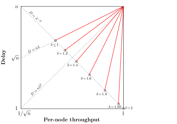
Figure 2: Delay-Throughput scaling trade-off (in log-log scale) for different values of $\delta$ between 0 and 2 (fast mobility case). The marks on the axes represent the orders asymptotically in $n$.

We now provide an intuitive explanation of the above results. Our schemes exploit node heterogeneity by an intelligent selection of relay nodes based on the location of their home-points. Essentially, we adopt a geographical routing strategy combined with a divide-and-conquer technique. Data are forwarded along a chain of relay nodes whose home-points progressively close in on the home-point of the destination. At each step, the distance between the home-point of the next-hop relay and the home-point of the target is halved, guaranteeing that the message is delivered to the destination in $\log{n}$ steps. Now, at a given point in space the density of nodes whose home-points are at distance $O(Z)$ from the pointgrows as $Z^{2}Z^{-\delta}/G$. Therefore, for $\delta<2$ a node most frequently gets in contact with nodes whose home-point reside far way in the network area. As a consequence, for $\delta<2$ the critical step for the system performance is the last one, in which the packet has to advance by the minimum distance along the chain of home-points. Instead, for $\delta>2$ a node typically gets in contact with nodes whose home-point are close to the home-point of the node. As a consequence, for $\delta>2$ the critical step for the system performance is the first one, in which the packet has to advance by the maximum distance along the chain of home-points. The value $\delta=2$ is the unique exponent at which the home-points of the nodes encountered by a given node are equally distributed at all distance scales. As a consequence, no step is critical and the system achieves the optimal performance both in terms of throughput and delay.

We remark that our system presents an interesting analogy with the problem of navigating small-world graphs using decentralized algorithms employing only local contact information. In particular we mention here a well known result due to J. Kleinberg [23], who studied a 2-dimensional lattice enriched by random shortcuts according to a probability which decays as a power law with the distance between the connected vertices. The number of hops required to reach an arbitrary destination exhibits a behavior similar to that in Figure 1 as a function of the power-law exponent. In particular, a unique value of the exponent (equal to 2) allows to navigate the graph in $\log{n}$ hops.

5 Fast mobility: scheduling-routing schemes

In this section we describe the scheduling-routing schemes that we have devised for our system, in the case of fast mobility. They form a family of schemes because one parameter, $Z_{0}$, is free, and can be specified within a particular scheme so as to achieve a desired delay-throughput trade-off.

Before going on we premise a useful concentration result widely used in previous work.

Lemma 1

Let ${\cal T}$ be a tessellation of ${\cal O}$, whose elements $T_{i}$ have area $|T_{i}|$. The number of home-points falling within each ${T}_{i}$ is, with high probability, $\Theta(|T_{i}|)$, uniformly over ${\cal O}$, as long as $|T_{i}|=\Omega(\log n)$, $\forall i$.

We do not repeat the proof of this lemma, which is based on a standard application of the Chernoff bound (see [24]).

5.1 Routing schemes

As already mentioned, we propose a bisection technique that makes messages advance along a chain of relay nodes whose home points become progressively closer to the home point of the destination. We stop the bisection when the home-point of the target node falls within distance $Z_{0}$ from the home-point of the last relay node.

To formalize this idea, suppose that node $a$ handles a message $m$ directed to $d$. Node $a$ first computes $d^{H}_{ad}=||H_{a}-H_{d}||$; if $d^{H}_{ad}\leq Z_{0}$ node $a$ directly forwards the message to node $d$ at the first transmission opportunity among the two nodes (as dictated by the scheduling scheme).

If $d^{H}_{ad}>Z_{0}$, node $a$ compares $d^{H}_{ad}$ with the set of thresholds $\{Z_{i}=2^{i}Z_{0},\;i\in{\mathbb{N}}\}$, finding the $i^{*}\geq 1$ such that, $2^{i^{*}-1}Z_{0}<d^{H}_{ad}<2^{i^{*}}Z_{0}$. In this case node $a$ is allowed to forward the message to any node $b$ whose home-point satisfies the following geometric constraint with respect to the home-point of $d$: $2^{i^{*}-2}Z_{0}<d^{H}_{bd}<\gamma~{}2^{i^{*}-1}Z_{0}$, where $1/2<\gamma<1$ is a constant introduced to simplify the analysis of our schemes. For the sake of concreteness, in the following we will consider the special case of $\gamma=3/4$. However, notice that asymptotic results are, in order sense, insensitive to $\gamma$. While being handled by $a$, we say that message $m$ is in step $i^{*}$ of the routing algorithm. Note that steps are counted backward starting from the destination, and that message $m$ has to go through $i^{*}$ relay nodes before being delivered to the destination.

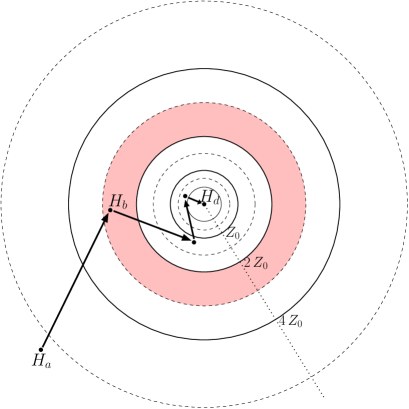
Figure 3: Example of routing of a message from $a$ to $d$. Dots denote home-points of the nodes.

As an example, consider the case illustrated in Figure 3, in which source node $a$ wants to send a message to node $d$. Distance $d^{H}_{ad}$ between the home-points of $a$ and $d$ satisfies $4Z_{0}<d^{H}_{ad}<8Z_{0}$, hence we have $i^{*}=3$. This means that message $m$ is in step 3 of the routing algorithm, thus it has to go through 3 relay nodes before being delivered to the destination. Since in this case $2^{i^{*}-2}Z_{0}=2Z_{0}$ and $\frac{3}{4}2^{i^{*}-1}Z_{0}=3Z_{0}$, the home-points of the nodes $b$ to which $a$ can forward the message have to lie in the ring $2Z_{0}<d^{H}_{bd}<3Z_{0}$, which is depicted in Figure 3 as a shaded region.

5.2 Scheduling schemes

A scheduling scheme is in charge of selecting, at each slot, the set of (non-interfering) transmitter-receiver pairs to be enabled in the network, as well as the message to be transmitted over each enabled pair. In our family of schemes, the transmission range employed by a transmitter depends on the routing step reached by the message to be sent. To better pack simultaneous transmissions, and thus maximize the network throughput, our scheduling policy selects, in a given slot, transmissions having homogeneous transmission ranges. This is done by selecting, at the beginning of each slot, a step $i$ according to an assigned probability distribution $p^{s}_{i}$. Then the slot is reserved only to messages which are in step $i$ of the routing algorithm, i.e., to messages currently stored at nodes whose home-points are at distances ranging between $2^{i-1}Z_{0}$ and $2^{i}Z_{0}$ from the home-point of the destination (for the particular case $i=0$, distances are between $0$ and $Z_{0}$).

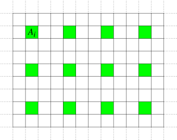
Figure 4: Example of non-interfering subset of squarelets with $M=9$.

A common transmission range $R_{i}$ is employed by all communications occurring during a slot devoted to step $i$. Once step $i$ has been selected, the domain ${\cal O}$ is divided into squarelets of area $A_{i}=R_{i}^{2}$, forming a regular square tessellation. According to the protocol model, at most one transmission can be enabled in each squarelet. Moreover, one can easily construct $M=\Theta(1)$ subsets of regularly spaced, non-interfering squarelets (for example, $M=9$ assuming a protocol model with $\Delta=0$, see Figure 4). Each subset can then be enabled in one out of $M$ slots, guaranteeing fairness among all squarelets and absence of interference among concurrent transmissions.

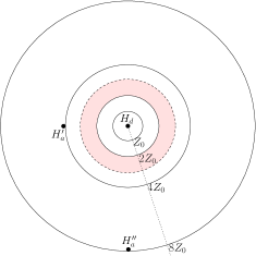
(a) Examples of locations of $H_{a}$ at routing step 3, given $H_{d}$

(b) Examples of locations of $H_{d}$ at routing step 3, given $H_{a}$. The shaded regions around $H^{\prime}_{d}$ and $H^{\prime\prime}_{d}$ denote the corresponding locations of $H_{b}$

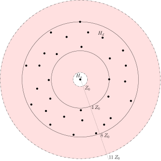
(c) The shaded region denotes the union of all possible locations of $H_{b}$ at routing step 3

Figure 5: Geometric considerations supporting the proposed scheduling schemes

Within a given squarelet ${\cal S}$, the specific transmitter-receiver pair $(a,b)$ to be enabled is selected as follows.

In slots devoted to the last step ($i=0$), first all pairs $(a,d)$ residing in ${\cal S}$ and such that: i) $d^{H}_{ad}<Z_{0}$; ii) $a$ has some message $m$ destined to $d$, are first classified as eligible for transmission. Then, if the set of eligible pairs is not empty, the squarelet ${\cal S}$ is declared as active and one pair is randomly selected for transmission. Notice that, provided that $Z_{0}=\Omega(\sqrt{\log n})$, by Lemma 1, each node has w.h.p. $\Theta(Z_{0}^{2})$ destinations $d$.

In slots devoted to step $i>0$, first each node $a$ residing in ${\cal S}$ selects a message $m$ from its buffer, which has reached step $i$ (if there is any); let $d_{m}$ be the final destination of message $m$. All pairs of nodes $(a,b)$ residing in ${\cal S}$ and such that: i) $a$ has selected one message $m$; ii) $b$ can act as ($i\!-\!1$)-th relay for message $m$, are first classified as eligible for transmission. Then, if the set of eligible pairs is not empty, the squarelet ${\cal S}$ is declared as active and one pair is randomly selected for transmission. We further assume that message $m$ is selected by node $a$ according to a FIFO scheduling policy.

Thus, logically each node is equipped with a FIFO queue for each step $i$, $i\geq 1$, plus one queue per destination for step 0, in which messages are sent directly to the target node (see Figure 6).

An illustration of how our scheduling scheme works is reported in Fig. 5. Suppose, as an example, that the current slot has been assigned to step $i^{*}=3$. Then we have a situation similar to the one already considered in Figure 3 while describing the routing scheme. Figure 5(a) shows, for a given destination home-point $H_{d}$, two possible locations $H^{\prime}_{a}$ and $H^{\prime\prime}_{a}$ for the home-point of the transmitting node $a$. In particular, $H^{\prime}_{a}$ ($H^{\prime\prime}_{a}$) is characterized by the smallest (largest) distance from $H_{d}$. If we now take the point of view of a given transmitting node $a$, we obtain the symmetric situation depicted in Figure 5(b), in which $H^{\prime}_{d}$ ($H^{\prime\prime}_{d}$) are located at the smallest (largest) distance from $H_{a}$. The shaded ring around $H^{\prime}_{d}$ ($H^{\prime\prime}_{d}$) denotes the possible location of the home-point $H_{b}$ of feasible relay nodes for the corresponding destination. Notice that, by selecting the head-of-the-line message, we constrain ourselves to a given destination home-point, and thus we can only use relay nodes whose home-points lie within a ring similar to the ones depicted in Figure 5(b).

In Figure 5(c) we have shown the union of all of the possible rings of the type shown in Figure 5(b), as we let the location of $H_{d}$ vary. The union region comprises all nodes $b$ satisfying $\frac{Z_{i}}{8}\leq d^{H}_{ab}\leq\frac{11}{8}Z_{i}$, for the generic step $i\geq 1$.

Notice again that, provided that $Z_{i}=\Omega(\sqrt{\log n})$, by Lemma 1 there are w.h.p. $\Theta(Z_{i}^{2})$ nodes $b$ which may potentially act as relay node, and all of them are at distance $\Theta(Z_{i})$ from $a$. Moreover, the same is true if we constrain ourselves to a given destination home-point (the area of any shaded ring as in Figure 5(b) is $\Theta(Z_{i}^{2})$, and all of its point are at distance $\Theta(Z_{i})$ from $a$). This observation already suggests that our policy can obtain the same asymptotic performance (in order sense) as the one achievable by a more aggressive scheduling policy which selects the message to transmit based on the availability of next-step relays in the same squarelet of the transmitter. This intuition will be confirmed later in our analysis.

In the following, we will always assume that $Z_{0}$ (and thus all $Z_{i}$’s) are $\Omega(\sqrt{\log n})$, so that we can apply the concentration result in Lemma 1.

6 Analysis of the proposed schemes

6.1 Design considerations

Given that step $i$ has been selected at the beginning of a slot, by construction the number $N_{i}$ of parallel transmissions that can occur in the network during the slot equals the number of active squarelets. On average we have:

$$E[N_{i}]=\frac{n}{MA_{i}}\Pr\{\mbox{active squarelet}\mid i\}$$ (2)

where $n$ is the total network area, $M$ is a finite constant accounting for interference (see 5.2) and $\Pr\{\mbox{active squarelet}\mid i\}$ is the probability that a generic squarelet ${\cal S}$ is active at step $i$.

From the discussion in Section 5.2, a squarelet ${\cal S}$ is active if the following two conditions hold: i) at least one pair $(a,b)$ of nodes is found within ${\cal S}$, such that $b$ can act at as ($i\!-\!1$)-th relay node for $a$ ($i\geq 1$), i.e., $\frac{Z_{i}}{8}\leq d^{H}_{ab}\leq\frac{11}{8}Z_{i}$ (in the case $i=0$, $b$ must be a destination node satisfying $\frac{Z_{0}}{2}\leq d^{H}_{ab}\leq\frac{3}{4}Z_{0}$); ii) node $a$ has a message to transmit to node $b$ (recall that, for $i\geq 1$, only the head-of-the-line message in the queue associated to step $i$ can be transmitted).

We observe that the probability that condition i) above holds, denoted by $\Pr\{\mbox{populated squarelet}\mid i\}$, depends only on the geometry of nodes and on the mobility process, not on the traffic (i.e., queues dynamics). In general we have

$$\Pr\{\mbox{active squarelet}\mid i\}\leq\Pr\{\mbox{populated squarelet}\mid i\}$$

The choice of $A_{i}$ is critical. The selection of a too large value for $A_{i}$ leads to a suboptimal exploitation of spatial reuse (thus causing throughput degradation), without being effective in reducing the delivery delay. This is because of the contention delay among many eligible transmitter-receiver pairs $(a,b)$ residing in squarelet ${\cal S}$ (recall that only one of them can be enabled), which offsets the advantage of reaching a more distant receiver in a single slot.

On the other hand, the selection of a too small value for $A_{i}$ is ineffective in terms of throughput (and also in terms of delay). This is because the potential benefit of increasing the spatial reuse is countered by the fact that the fraction of active squarelets tends to 0.

Therefore, a reasonable design choice is to minimize the squarelet size $A_{i}$ under the constraint that:

$$\liminf_{n\to\infty}\Pr\{\mbox{populated squarelet}\mid i\}>0$$

Although this criterion provides only an upper bound to the probability that a squarelet is active, we will later show in Section 6.5 that the network queues can be loaded, under our schemes, in such a way that the probability that node $a$ indeed has a message to transmit to $b$ is also w.h.p. greater than zero.

We will further assume that $\sqrt{A_{i}}=R_{i}=O(Z_{i})$; i.e., the transmission range used at step $i$ should be smaller than or equal (in order sense) to the distance between the home-points of the transmitter and the receiver. This because it does not make sense to use a transmission range larger (in order sense) than the distance gained along the chain of home-points followed by the routing algorithm (otherwise the same transmission range could be used in a previous step to directly reach the destination, as done in the last step).

The following lemma will be useful for dimensioning $A_{i}$.

Lemma 2

At routing step $i$, the minimum value of $A_{i}$ which guarantees that $\liminf_{n\to\infty}\Pr\{\mbox{populated squarelet}\mid i\}>0$ is given by:

$$A_{i}=\left\{\begin{array}[]{cc}\Theta\left(\frac{n^{1/2}}{Z_{i}}\right)&\delta\leq 1\\ \Theta\left(\frac{n^{\frac{2-\delta}{2}}}{Z_{i}^{2-\delta}}\right)&1<\delta<2\\ \Theta\left(\log n\right)&\delta=2\\ \Theta\left(Z_{i}^{{\delta-2}}\right)&\delta>2\\ \end{array}\right.$$ (3)

(see Appendix A).

We observe that $A_{i}$ depends both on the value $Z_{i}=2^{i}Z_{0}$ of the associated routing step and on the power law exponent $\delta$ which characterizes node mobility.

For $\delta<2$ the largest value of $A_{i}$ corresponds to the last step (i.e., step 0, having minimum $Z_{i}$ equal to $Z_{0}$). In this case, $Z_{0}$ cannot be chosen arbitrarily small. In particular, for any $\delta\leq 1$, condition $\sqrt{A_{i}}=R_{i}=O(Z_{i})$, coupled with (3), implies that $Z_{0}=\Omega(n^{1/6})$. For $1<\delta<2$, the same condition implies that $Z_{0}=\Omega\left(n^{\frac{2-\delta}{8-2\delta}}\right)$.

For $\delta=2$, $A_{i}$ does not depend on $Z_{i}$, therefore the same transmission range $R=\sqrt{\log{n}}$ can be used in all steps. Notice that $R_{i}=O(Z_{i})$ is satisfied because we require that $Z_{0}=\Omega(\sqrt{\log n})$.

For $\delta>2$ the first step (having the maximum $Z_{i}$) is the one that requires the largest value of $A_{i}$. Also in this case, to apply Lemma 1, we require that $Z_{0}=\Omega(\sqrt{\log n})$.

To summarize, the conditions on the free parameter $Z_{0}$ of our class of scheduling-routing schemes are the following:

$$Z_{0}=\left\{\begin{array}[]{cc}\Omega\left(n^{1/6}\right)&\delta<1\\ \Omega\left(n^{\frac{2-\delta}{8-2\delta}}\right)&1\leq\delta<2\\ \Omega(\sqrt{\log n})&\delta\geq 2\end{array}\right.$$ (4)

At last, we need to dimension the probability distribution $p^{s}_{i}$ with which slots are assigned to the different steps of the routing algorithm. A natural choice is to equalize of the average number of transmissions that can occur for each step, and thus avoid that a particular step becomes the system bottleneck. This is obtained by making $p^{s}_{i}$ inversely proportional to $\overline{N}_{i}=\frac{n}{A_{i}}$, which is an upper bound to the average number of parallel transmissions $E[N_{i}]$ at step $i$.

Given that $i_{\max}=\lfloor\frac{1}{2}\log_{2}n-\log_{2}Z_{0}\rfloor$ is the maximum number of steps traversed by messages, using (2) we have

$$p^{s}_{i}=\frac{\frac{1}{\overline{N}_{i}}}{\sum_{i=0}^{i_{\max}}\frac{1}{\overline{N}_{i}}}=\frac{A_{i}}{\sum_{i=0}^{i_{\max}}A_{i}}$$ (5)

We will later see that this choice of $p^{s}_{i}$ indeed equalizes the average number of parallel transmissions occurring at each step.

6.2 A first throughput characterization

An upper-bound to the network throughput achievable by our scheduling-routing schemes can be easily computed in terms of the maximum number of messages that can flow in one slot from the sources to the destinations, under the optimistic hypothesis that

$$\Pr\{\mbox{active squarelet}\mid i\}=\Pr\{\mbox{populated squarelet}\mid i\}$$

Considering a particular step $i$, the average number of messages stored at $i$-th relay nodes which can advance to ($i\!-\!1$)-th relay nodes (or be delivered to the destinations, in the case $i=0$) in one slot is bounded by $p^{s}_{i}\overline{N_{i}}$. It follows that an upper-bound to the network throughput $\Lambda$ is expressed by:

$$\overline{\Lambda}=n~{}\overline{\lambda}=\min_{i}(p^{s}_{i}\overline{N}_{i})$$ (6)

Given the design choice (5) we obtain:

$$\overline{\Lambda}=p^{s}_{0}\overline{N}_{0}=\frac{n}{\sum_{i=0}^{i^{\max}}A_{i}}$$

For $\delta\leq 1$, being $A_{i}=\frac{n^{1/2}}{Z_{i}}$, it follows:

$$\overline{\Lambda}=\frac{n}{\sum_{i=0}^{i_{\max}}\frac{n^{1/2}}{(2^{i}Z_{0})}}=\Theta(n^{\frac{1}{2}}Z_{0})$$ (7)

For $1<\delta<2$, being $A_{i}=\frac{n^{\frac{2-\delta}{2}}}{Z_{i}^{2-\delta}}$, it follows:

$$\overline{\Lambda}=\frac{n}{\sum_{i=0}^{i_{\max}}\frac{n^{\frac{2-\delta}{2}}}{(2^{i}Z_{0})^{2-\delta}}}=\Theta(n^{\frac{\delta}{2}}Z_{0}^{2-\delta})$$ (8)

For $\delta=2$, let $Z_{0}=n^{\beta}$. We have:

$$\overline{\Lambda}=\frac{n}{\sum_{i=0}^{i_{\max}}\log n}=\left\{\begin{array}[]{cc}\Theta(\frac{n}{\log^{2}(n)})&\quad\,\beta<1/2\\ \Theta(\frac{n}{\log n})&\quad\,\beta=1/2\end{array}\right.$$ (9)

At last in the case $\delta>2$

$$\overline{\Lambda}=\frac{n}{\sum_{i=0}^{i_{\max}}(2^{i}Z_{0})^{{\delta-2}}}=\frac{n}{n^{\frac{{\delta-2}}{2}}}\dfrac{1}{\sum_{i=0}^{i_{\max}}{(2^{{2-\delta}}})^{i}}=\Theta(n^{2-\frac{\delta}{2}})$$ (10)

6.3 Delay analysis

Now we turn our attention to the delay. We consider a generic node $a$ which is storing a message $m$ in step $i$, directed to final destination $d$. We need to evaluate the average number of slots needed to make this message advance by one step. By so doing we neglect the effects of possible contention for transmission among different messages in step $i$ stored at node $a$; this is equivalent to ignoring queueing delays within each node, and considering only the service time (we will analyze queueing effects in Section 6.4).

Node $a$ is enabled to transmit message $m$ in a given slot if the following three conditions hold: i) the slot is assigned to the $i$-th step; ii) an eligible relay node $b$ for the head-of-the-line message of the queue devoted to step $i\geq 1$, or a suitable destination node $d$ (for step $i=0$), is found in the same squarelet in which $a$ resides; iii) among all the eligible contending pairs residing in the same squarelet, a pair is selected in which $a$ acts as transmitter. The occurrence of condition i) is simply $p^{s}_{i}$. The probability $p^{\alpha}_{i}$ of the occurrence of condition ii) is computed in Appendix B:

$$p^{\alpha}_{i}=\left\{\begin{array}[]{cc}\Theta\left(A_{i}\frac{|\Gamma_{i}|}{n}\right)&\delta\leq 1\vspace{1mm}\\ \Theta\left(A_{i}\frac{Z_{i}^{2(1-\delta)}|\Gamma_{i}|}{n^{2-\delta}}\right)&1<\delta<2\vspace{1mm}\\ \Theta\left(A_{i}\frac{|\Gamma_{i}|}{Z_{i}^{2}}\frac{\log Z_{i}}{\log^{2}n}\right)&\delta=2\\ \Theta\left(A_{i}|\Gamma_{i}|Z_{i}^{-\delta}\right)&\delta>2\\ \end{array}\right.\vspace{-1mm}$$ (11)

In the above expressions, $|\Gamma_{i}|$ denotes the number of potential receivers of message $m$ that exist in the network. For $i>0$, we have $|\Gamma_{i}|=\Theta(Z^{2}_{i})$, whereas in the last step there exists a unique receiver (i.e., the destination), hence $|\Gamma_{0}|=1$.

The probability $p^{\beta}_{i}$ of the occurrence of condition iii) depends on the value of $\delta$. For $\delta<2$, $p^{\beta}_{i}=\Theta(1)$, because the average number $E[N^{\cal S}_{(ab)}]$ of eligible contending pairs $(a,b)$ that can be found in a squarelet is finite (see Appendix A) and by Jensen inequality we have $p^{\beta}_{i}>E[1/N^{\cal S}_{(ab)}]>1/E[N^{\cal S}_{(ab)}]=\Theta(1)$. For $\delta\geq 2$, instead, there is an infinite number $N^{\cal S}_{a}$ of transmitting nodes $a$ and a finite number $N^{\cal S}_{b}$ of receiving nodes $b$ (see Appendix A). Therefore, under the pessimistic assumption that all nodes $a$ have a packet to transmit, it follows $p^{\beta}_{i}>E[1/N^{\cal S}_{a}]>1/E[N^{\cal S}_{a}]$. We have,

$$p^{\beta}_{i}=\left\{\begin{array}[]{cc}\Theta(1)&\delta<2\\ \Omega\left(\frac{\log n}{A_{i}\log A_{i}}\right)&\delta=2\\ \Omega(1/A_{i})&\delta>2\end{array}\right.\vspace{-1mm}$$ (12)

The probability $p^{T}_{i}$ that $a$ transmits message $m$ in a given slot can then be computed as $p^{T}_{i}=p^{s}_{i}p^{\alpha}_{i}p^{\beta}_{i}$:

$$p^{T}_{i}=\left\{\begin{array}[]{cc}\Theta\left(\frac{|\Gamma_{i}|Z_{0}}{n^{\frac{1}{2}}Z_{i}^{2}}\right)&\delta\leq 1\\ \Theta\left(\frac{|\Gamma_{i}|Z_{0}^{2-\delta}}{Z_{i}^{2}n^{1-\frac{\delta}{2}}}\right)&1<\delta<2\\ \Omega\left(\frac{|\Gamma_{i}|\log Z_{i}}{Z_{i}^{2}\log^{3}(n)\log\log n}\right)&\delta=2\\ \Omega\left(\frac{|\Gamma_{i}|}{Z_{i}^{2}n^{\frac{\delta}{2}-1}}\right)&\delta>2\\ \end{array}\right.\vspace{-1mm}$$ (13)

At last, under the pessimistic assumption that all nodes in the network are constantly backlogged by messages in step $i$, the chances that message $m$ is forwarded in a slot form a memoryless Bernoulli process, since $p^{T}_{i}$ depends only on the geometry of nodes, which completely regenerates at every slot. Thus, it immediately follows that the average service time $D_{S}^{i}$ of a message in step $i$ is equal to $1/p^{T}_{i}$. Neglecting queueing delays, the total delay $D_{S}$ from source to destination can be computed as $D_{S}=\sum_{i}D_{S}^{i}$. It follows:

$$D_{S}=\left\{\begin{array}[]{cc}\Theta(Z_{0}n^{\frac{1}{2}})&\delta\leq 1\\ \Theta(Z_{0}^{\delta}n^{1-\frac{\delta}{2}})&1\leq\delta<2\\ O(\frac{Z_{0}^{2}\log^{3}(n)\log\log n}{\log Z_{0}})&\delta=2\\ O(n^{\delta/2-1}Z^{2}_{0})&\delta>2\end{array}\right.\vspace{-1mm}$$ (14)

6.4 The effect of traffic

In the above computation we have assumed that the delay experienced by a message at a node is of the same order of magnitude as the service time, i.e., the time that elapses from when the message becomes head-of-the-line to when it is successfully transmitted. This can be justified by Kingman’s upper bound to the total delay of a discrete-time GI/GI/1-FIFO queue [25], which states that as long as the second moment $\sigma^{2}_{a}$ of the number of simultaneous arrivals is finite, the second moment $\sigma^{2}_{D}$ of service time is also finite and the queue-load $\rho$ is strictly less than one, the average queueing delay $D^{i}$ is bounded by:

$$D^{i}\leq D^{i}_{S}\max\left(1,\frac{\sigma^{2}_{a}+\sigma^{2}_{D}}{2(D^{i}_{S})^{2}(1-\rho)}\right)$$

from which it follows that $D^{i}=\Theta(D^{i}_{S})$. In our case the fact that $\sigma^{2}_{a}<\infty$ is immediate in light of the fact that at most one message can be enqueued per slot at any node, while $\sigma^{2}_{D}<\infty$ derives from the fact that the service time distribution is stochastically dominated by a geometric distribution.

6.5 Maximum Throughput evaluation

We observe that the whole system can be represented by an acyclic network of GI/GI/1-FIFO queues; indeed messages advance in the network visiting queues associated to decreasing step indices $i$, which guarantees the absence of loops (see Figure 6). As a consequence, offered traffic $\Lambda$ can be successfully transferred through the network, as long as no queue is overloaded.

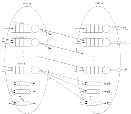
Figure 6: Internal architecture of the nodes: queue structure

The stability condition for the single FIFO queue present at each node $a$, which stores messages belonging to step $i\geq 1$ of the routing algorithm, is $\lambda^{a}_{i}<p_{i}^{T}$, where $\lambda^{a}_{i}$ is the aggregate arrival rate of messages in step $i$ at node $a$, while $p_{i}^{T}$ is the transmission probability computed in Section 6.3.

Considering the last step (i=0), since in this case messages directed to different destinations are stored in separate queues, the stability condition for the generic queue storing messages directed to destination $d$ is $\lambda_{0}^{ad}<p_{0}^{T}$, being $\lambda_{0}^{ad}$ the arrival rate at node $a$ of last-step messages directed to $d$.

Substituting the expression for $p_{i}^{T}$, we immediately obtain that the maximum traffic sustainable by node queues satisfies:

$$\lambda^{a}_{i}=\Theta(\overline{\lambda})\qquad i\geq 1\vspace{-1mm}$$

and

$$\lambda^{ad}_{0}=\Theta\left(\frac{\overline{\lambda}}{Z_{0}^{2}}\right)$$

i.e., every node $a$ can sustain, for each step, a traffic $\Theta(\overline{\lambda})$, expressed in messages per slot (in the case of step $i=0$, recall that every node w.h.p. delivers last-step messages to $\Theta(Z_{0}^{2})$ different destinations).

Note that our scheduling-routing scheme w.h.p. distributes the network traffic uniformly (in order sense) among all network nodes. We conclude that the sustainable network throughput is w.h.p. $\Theta(\overline{\Lambda})$, i.e., the upper bounds previously computed in Section 6.2 are asymptotically tight.

We remark that this last finding implies that: i) no step becomes the system bottleneck under our choice of slot assignment probabilities $p^{s}_{i}$; ii) if the network sustains a throughput $\Theta(\Lambda)$, necessarily $\Pr\{\mbox{active squarelet}\mid i\}=\Theta(\Pr\{\mbox{populated squarelet}\mid i\})$.

At last, we can claim the optimality of our scheduling-routing schemes for $\delta<2$. This in light of the following proposition.

Proposition 1

Consider any scheduling-routing scheme according to which messages are delivered to destinations $d$ by nodes $a$ whose home-points satisfy $d^{H}_{ad}=\Theta(Z)$, employing a transmission range $R$. Then, necessarily the network throughput is $\Lambda=O(\frac{n}{R^{2}})$. In addition, if no message replication is employed, the delay is $D=\Omega\left(1/{\Pr\{\mbox{meet}\}}\right)$, where $\Pr\{\mbox{meet}\}$ is the probability that any two nodes $(a,d)$, with $d^{H}_{ad}=\Theta(Z)$, fall within the transmission range of each other.

The throughput condition is an immediate consequence of the protocol interference model, that prevents two nodes whose relative distance is smaller than $\frac{\Delta}{2}R$ from transmitting simultaneously [1]. The delay condition immediately descends from the observation that $a$ can deliver a message to $d$, only if $d$ falls within the transmission range of $a$. Comparing the bounds of Proposition 1 with the performance achievable by our scheduling-routing schemes (for which $Z=Z_{0}$ and $R=\sqrt{A_{0}}$), we conclude that our schemes, for $\delta<2$, achieve optimal delay-throughput trade-offs within the class of algorithms that do not employ message replication.

6.6 Possible delay throughput trade-offs

Let us first examine the case $\delta>2$. According to (10) the system throughput does not depend on $Z_{0}$, whereas the delay (14) increases with $Z_{0}$. Thus, $Z_{0}$ should be minimized to reduce as much as possible the delay, while no delay-throughput trade-offs are possible. Recalling the condition (4) we set $Z_{0}=\sqrt{\log n}$ and obtain

$$\lambda=\Theta(n^{1-\delta/2})\qquad D=O(n^{\delta/2-1}\log n)$$

Also for $\delta=2$ the dependence of the throughput on $Z_{0}$ is weak, since any choice of $Z_{0}=O(n^{\beta})$, with $\beta<1/2$, leads to the same throughput, while a $\log n$ factor is gained selecting $Z_{0}=\Theta(n^{1/2})$, however at the expense of a severe increase of the delay. Hence it appears optimal to select $Z_{0}=\Theta{\sqrt{\log n}}$, resulting in:

$$\lambda=\Theta\left(\frac{1}{\log^{2}(n)}\right)\qquad D=O(\log^{4}(n))$$

For $\delta<2$, instead, different trade-offs between throughput (optimized selecting $Z_{0}$ large) and delay (minimized selecting $Z_{0}$ small) are possible. Let $Z_{0}=n^{\beta}$.

For $1<\delta<2$, being $\frac{2-\delta}{8-2\delta}\leq\beta\leq 1/2$, we obtain

$$\lambda=\Theta(n^{\delta/2-1+\beta(2-\delta)})\qquad D=\Theta(n^{1-\delta(1/2-\beta)})$$

whereas for $\delta\leq 1$, being $1/6\leq\beta\leq 1/2$, we obtain

$$\lambda=\Theta(n^{\beta-\frac{1}{2}})\qquad D=\Theta(n^{{\beta+\frac{1}{2}}})$$

6.7 Alternative scheme for large $\delta$

It should be noticed that the performance of our scheduling-routing schemes in the case of $\delta>2$ rapidly deteriorates in terms of both throughput and delay for large values of $\delta$. Therefore, we propose here an alternative scheme, valid for $\delta>2$, whose performance does not depend on $\delta$.

We observe that, for $\delta>2$, every node spends a constant fraction of time within a finite distance from its home-point. Hence it is possible to devise a scheduling-routing scheme which is based on this property and that does not exploit node mobility at all. The network area ${\cal O}$ is divided into a regular square tessellation whose elements have area equal to $\log{n}$. Within each squarelet, only the nodes whose home-points belong to the squarelet itself, are allowed to transmit or receive, using a fixed transmission range equal to $\sqrt{\log{n}}$. Since each node spends a constant fraction of time in the squarelet containing its home-point, the performance that we can achieve is the same as if nodes were fixed at their home-points, i.e., it is equivalent in order sense to the Gupta-Kumar case. We can therefore obtain a per node-throughput $\lambda=\Theta(1/\sqrt{n\log{n}})$ and delay $D_{S}=\Theta(\sqrt{n/\log{n}})$ [8].

A comparison with our previous scheduling-routing schemes leads to the conclusion that the alternative scheme becomes convenient for $\delta>3$ (see Figure 1).

7 The slow mobility case

In presence of slow mobility it is potentially possible to deliver messages along multi-hop paths in a single slot. Our goal is to understand whether this possibility can be exploited within our class of scheduling-routing schemes to further improve their performance.

A particular case, which serves as a lower bound on the system performance, is when there is a single step, characterized by $Z_{0}=\sqrt{n}$, for which the resulting scheme essentially degenerates to the Gupta-Kumar case, providing per-node throughput $\lambda=\Omega(1/\sqrt{n\log{n}})$ and delay $D_{S}=\Theta(1)$ (according to the new definition of slot).

Potentially better delay-throughput trade-offs could be achieved by employing a hybrid scheme in which messages are first routed according to the previously described bisection routing scheme, up to arriving at a critical distance from the destination (to be specified), and then transferred to the destination in just one slot over a multi-hop path. This means that when the last step ($i=0$) is scheduled, the network area is subdivided into squarelets of area $B_{0}=\omega(A_{0})$, and many (disjoint) multi-hop transmissions are established within each squarelet. This class of hybrid schemes may be effective for $\delta<2$., i.e., when performance is indeed limited by the last step. Therefore in the following analysis we assume $\delta<2$.

7.1 Analysis

We first analyze the throughput performance in the last step, considering the effect of multi-hop transmissions. Denoting by $Q(B_{0})$ the number of multi-hop transmissions that can be enabled in a squarelet of size $B_{0}$ during a slot, and by $\tilde{N}_{0}$ the total number of parallel transmissions occurring in the network at step 0, we have

$$E[\tilde{N}_{0}]=\frac{n}{B_{0}}E[Q(B_{0})]$$ (15)

In the previous bisection scheme, the squarelet size $A_{0}$ was dimensioned in such a way that a finite number of eligible transmitter-receiver pairs (single-hop) can be found in a squarelet of area $A_{0}$. Therefore, in a squarelet of area $B_{0}$ we have $C_{0}=\Theta(B_{0}/A_{0})$ nodes that can communicate among them over multi-hop paths. Although the number of pairs that can potentially be established increases quadratically with $B_{0}$, only $C_{0}$ of them are not conflicting (i.e., do not have a node in common). Therefore, we have $E[Q(B_{0})]=C_{0}=\Theta(B_{0}/A_{0})$. Plugging this expression in (15) we immediately see that $E[\tilde{N}_{0}]=E[{N}_{0}]=n/A_{0}$ for any choice of $B_{0}$, hence there is no advantage in terms of spatial reuse by using multi-hop paths.

Turning our attention to the delay of the last step, we consider a message $m$ stored at $a$ and destined to $d$. The probability $p_{0}^{\alpha}$ that the pair of nodes $(a,d)$ reside in the same squarelet of area $B_{0}$ is (see appendix B):

$$p_{0}^{\alpha}=\left\{\begin{array}[]{cc}\Theta(\frac{B_{0}}{n})&\delta\leq 1\vspace{1mm}\\ \Theta\Big{(}B_{0}\frac{Z_{0}^{2(1-\delta)}}{n^{2-\delta}}\Big{)}&1\leq\delta\leq 2\end{array}\right.$$

hence it increases linearly with $B_{0}$. However in this case the probability $p_{0}^{\beta}$ that $(a,d)$ is selected is $\Theta(1/C_{0})=\Theta(A_{0}/B_{0})$, because among all $\Theta(C_{0}^{2})$ pairs that can potentially be enabled only $\Theta(C_{0})$ are not conflicting. As a result, the product $p_{0}^{\alpha}p_{0}^{\beta}$ does not depend on $B_{0}$, therefore no gain in terms of delay is obtained by a scheme that attempts multi-hop transmissions at the last step. The only exception to previous arguments is represented by the case in which there is a single step, and thus the hybrid scheme degenerates to the Gupta-Kumar case.

A graphical representation of the network power achievable in the slow mobility case is reported in Figure 7.

Figure 7: Power $\lambda/D$ (in log scale) as a function of $\delta$ (slow mobility case).

We observe that our class of routing-scheduling schemes performs better than the degenerate case of Gupta-Kumar for values of $\delta$ comprised in the interval $[1.6,2.5]$.

8 Discussion

Although mainly of theoretical interest, we believe that our work can provide fundamental principles to design smart routing protocols for mobile ad-hoc networks exploiting the spatial diversity of the nodes. In particular, our bisection routing strategy appears to be an attractive solution as long as the spatial distribution of users follows a power law. Although there is strong experimental evidence that this is true in many context related to both human and vehicular mobility, the precise exponent of the power law needs to be carefully estimated, either through measurements or by an autonomous self-learning procedure. Indeed, two main regimes occur depending on the exponent value: for values smaller than 2, the larger delays are expected in the last hop, whereas above 2 the critical hop is the first one. To avoid large delays, this requires to increase the transmission range either at the end or at the beginning of the route, which is a rather new concept. In this paper we have not addressed a number of issues which are essential to translate our scheme into an implementable solution. In particular, the impact of more realistic mobility models, and the local dissemination of information about the home-points of the nodes. However, we believe that the above issues do not compromise the applicability of our results to a real setting. Finally, the idea of progressively narrowing the selection of relay nodes through a divide-and-conquer technique, based on the similarity of the mobility pattern of the nodes, could be an interesting design principle to apply in a wider sense than presented here. In this case, one has to evaluate the mixing degree of the nodes in terms of distance scale membership, having defined a suitable distance metric between the mobility pattern of two nodes.

9 Conclusions

Previous work on delay-throughput trade-offs in mobile ad hoc networks has mostly been done under the assumption that nodes are homogeneous and uniformly visit the network area. In this paper we have shown that this condition can be largely suboptimal. Restricted mobility, which is usually found in practice, can be exploited by intelligent scheduling-routing schemes which make use of the geographical information about the location most visited by a node. In particular, we have introduced a new class of scheduling routing schemes which significantly outperform all previously proposed schemes for a wide range of restricted mobility patterns.

Appendix A Dimensioning of $A_{i}$

We first focus on the last step ($i=0$). We consider all distinct pairs of nodes $(a,b)$ whose home-points satisfy $Z_{0}/2\leq||H_{a}-H_{b}||<3Z_{0}/4$.

Given a squarelet ${\cal S}$ of area $A_{0}$, whose center of mass is for simplicity placed at the origin, we first evaluate the average number $E[\hat{N}_{(a,b)}^{\cal S}|\bf H]$ of ‘far’ node pairs $(a,b)$ (i.e., pairs such that both $||H_{a}||>Z_{0}/4$ and $||H_{b}||>Z_{0}/4$) that fall within ${\cal S}$. We further assume $\sqrt{A_{i}}\leq cZ_{0}$ for some $c<1/4$.

Let us denote with $I(H_{a},H_{b})$ the function that returns 1 if $Z_{0}/2\leq||H_{a}-H_{b}||<3Z_{0}/4$ and both $||H_{a}||>Z_{0}/4$ and $||H_{b}||>Z_{0}/4$. By construction, it follows:

$$E[\hat{N}_{(a,b)}^{\cal S}|{\bf H}]=\frac{1}{2}\sum_{a}\sum_{b\neq a}\int_{X_{1}\in{\cal S}}\int_{X_{2}\in{\cal S}}\phi(H_{a}-X_{1})$$

$$\phi(H_{b}-X_{2})I(H_{a},H_{b}){\rm\,d}X_{1}{\rm\,d}X_{2}$$

Note that $E[N_{(a,b)}^{\cal S}|\bf H]$ is a random variable over the space of all the possible home-point locations ${\bf H}$. However, since $Z_{0}=\Omega(\sqrt{\log n})$, applying Proposition 1 it can be immediately proved that, for $n\to\infty$, with high probability, $E[N_{(a,b)}^{\cal S}|{\bf H}]=\Theta(E[N_{(a,b)}^{\cal S}])$, being $E[N_{(a,b)}^{\cal S}]=E_{\bf H}[E[N_{(a,b)}^{\cal S}]\mid{\bf H}]$ the number of pairs averaged over all possible instances of ${\bf H}$. Hence, we have:

$$E[\hat{N}_{(a,b)}^{\cal S}]=\frac{1}{2}\int_{X_{1}\in{\cal S}}\int_{X_{2}\in{\cal S}}\int_{H_{a}\in{\cal O}}\int_{H_{b}\in{\cal O}}\\ \phi(H_{a}-X_{1})\phi(H_{b}-X_{2})I(H_{a},H_{b}){\rm\,d}H_{a}{\rm\,d}H_{b}\asymp\\ \asymp\frac{A_{0}^{2}}{2}\int_{H_{a}\in{\cal O}}\int_{H_{b}\in{\cal O}}\phi(H_{a})\phi(H_{b})I(H_{a},H_{b}){\rm\,d}H_{a}{\rm\,d}H_{b}=\\ =A_{0}^{2}\int_{H_{a}\in{\cal O}}\int_{H_{b}\in{\cal O}:||H_{b}||>||H_{a}||}\phi(H_{a})\phi(H_{b})I(H_{a},H_{b}){\rm\,d}H_{a}{\rm\,d}H_{b}=\\ \!\!\!\!\!\!\!\!=\!A_{0}^{2}\!\!\int_{H_{a}\in{\cal O}:||H_{a}||\leq CZ_{0}}\int_{H_{b}\in{\cal O}:||H_{b}||>||H_{a}||}\phi(H_{a})\phi(H_{b})I(H_{a},H_{b}){\rm\,d}H_{a}{\rm\,d}H_{b}+\\ \!+A_{0}^{2}\!\!\int_{H_{a}\in{\cal O}:||H_{a}||>CZ_{0}}\int_{H_{b}\in{\cal O}:||H_{b}||>||H_{a}||}\phi(H_{a})\phi(H_{b})I(H_{a},H_{b}){\rm\,d}H_{a}{\rm\,d}H_{b}$$

where the last two terms, for large $C$, may be interpreted, respectively, as the contribution of pairs $(a,b)$ whose home-points are at distance $\Theta(Z_{0})$ and the contribution of pairs whose home-points are at distance $\omega(Z_{0})$.

The first term can be approximated by the integral

$$\!\!A_{0}^{2}\!\int_{H_{a}\in{\cal O}:Z_{0}/4<||H_{a}||<4Z_{0}}\!\int_{H_{b}\in{\cal O}:||H_{b}||>||H_{a}||}\phi^{2}(Z_{0})I(H_{a},H_{b}){\rm\,d}H_{a}{\rm\,d}H_{b}=\\ =\Theta\Big{(}A_{0}^{2}\phi^{2}(Z_{0})Z_{0}^{4}\Big{)}$$

since, by triangular inequality, it must hold that:
$||H_{b}||<||H_{a}-H_{b}||-||H_{a}||=(C+1)Z_{0}$

The second term instead provides a contribution

$$\Theta\Big{(}A_{0}^{2}Z_{0}^{2}\int_{H_{a}\in{\cal O}:||H_{a}||>CZ_{0}}\phi^{2}(H_{a}){\rm\,d}H_{a}\Big{)}$$

Substituting the expression for $\phi(X)$, we obtain that the number of ‘far’ node pairs is:

$$E[\hat{N}_{(a,b)}^{\cal S}]=\left\{\begin{array}[]{cc}\Theta(\frac{A^{2}_{0}Z^{2}_{0}}{n})&\delta\leq 1\\ \Theta(\frac{A^{2}_{0}Z_{0}^{2(2-\delta)}}{n^{2-\delta}})&1<\delta<2\\ \Theta(\frac{A^{2}_{0}}{\log^{2}n})&\delta=2\\ \Theta(A^{2}_{0}Z_{0}^{2(2-\delta)})&\delta>2\\ \end{array}\right.$$

To ensure that a far pair $(a,b)$ is found within ${\cal S}$ with a non-vanishing probability it is necessary to dimension $A_{0}$ in such a way that $E[\hat{N}_{(a,b)}^{\cal S}]$ is not vanishing as $n\to\infty$. On the other hand making $E[\hat{N}_{(a,b)}^{\cal S}]=\Theta(1)$ is also sufficient to guarantee that a far pair is found within squarelet ${\cal S}$ with non vanishing probability.

Now we turn our attention to ‘near’ pairs, i.e., pairs of nodes $(a,b)$ in which one of the two nodes (let it be node $a$) has home-point satisfying: $||H_{a}||<Z_{0}/4$. First, note that by triangular inequality it must be $Z_{0}/4<||H_{b}||<Z_{0}$.Thus to find a ‘near’ pair $(a,b)$ within ${\cal S}$ with finite probability, we must find within ${\cal S}$ at least one node $a$ whose home-point satisfies $||H_{a}||<Z_{0}/4$ and at least one node $b$ whose home-point satisfies $Z_{0}/4<||H_{b}||<Z_{0}$.

The average number $E[N_{a}]$ of near nodes $a$ in squarelet ${\cal S}$ can be evaluated as:

$$\!E[N_{a}]\!\asymp\!A_{0}\!\int_{H_{a}\in{\cal O}:||H_{a}||<\frac{Z_{0}}{4}}\phi(H_{a}){\rm\,d}H_{a}=\left\{\begin{array}[]{cc}\Theta(\frac{A_{0}Z_{0}^{2-\delta}}{n^{\frac{2-\delta}{2}}})&\delta<2\\ \Theta(A_{0}\frac{\log Z_{0}}{\log n})&\delta=2\\ \Theta(A_{0})&\delta>2\\ \end{array}\right.$$

whereas the average number $E[N_{b}]$ of nodes $b$ within ${\cal S}$, such that $1/4Z_{0}<||H_{b}||<5/4Z_{0}$, is

$$\!\!\!E[N_{b}]\!\asymp\!A_{0}\!\!\int_{H_{b}\in{\cal O}:\frac{Z_{0}}{4}<||H_{b}||<Z_{0}}\phi(H_{b}){\rm\,d}H_{b}=\left\{\begin{array}[]{cc}\Theta(\frac{A_{0}Z_{0}^{2-\delta}}{n^{\frac{2-\delta}{2}}})&\delta<2\vspace{1mm}\\ \Theta(\frac{A_{0}}{\log n})&\delta=2\\ \Theta(A_{0}Z_{0}^{2-\delta})&\delta>2\\ \end{array}\right.$$

In order to have near pairs within squarelet ${\cal S}$ with a non vanishing probability, both $E[N_{a}]$ and $E[N_{b}]$ must be non vanishing. At last, $A_{0}$ must be dimensioned in such a way that either both $E[N_{a}]$ and $E[N_{b}]$ are non-vanishing, or $E[\hat{N}_{(a,b)}^{\cal S}]$ is non-vanishing, leading to the expressions in (3). for $i=0$.

Now turning our attention to the case $i>0$, we have to evaluate the average number of distinct pair of nodes $(a,b)$, whose home-point satisfy $\frac{1}{8}Z_{i}\leq||H_{a}-H_{b}||\leq\frac{11}{8}Z_{i}$, falling within a squarelet ${\cal S}$ of area $A_{i}$, whose center of mass is for simplicity placed at the origin.

This can be done using exactly the same approach as before, i.e., distinguishing between ‘far’ node pairs $(a,b)$ (pairs such that both $||H_{a}||\geq Z_{i}/16$ and $||H_{b}||\geq Z_{i}/16$) and ‘near’ node pairs (pairs $(a,b)$ in which at least one of the two nodes (let it be node $a$) has the home-point satisfying $||H_{a}||<Z_{i}/16$), and evaluating separately the two contributions.

Appendix B Evaluation of $p^{\alpha}_{i}$

Consider a pair of nodes $a$ and $b$ such that $||H_{a}-H_{b}||=D$. We wish to evaluate (in order sense) the probability $p_{(a,b)}$ that $(a,b)$ are found within the same squarelet ${\cal S}$ of area $A$:

$$\@ADDCLASS{ltx_eqn_lefteqn}$\displaystyle p_{(a,b)}=\sum_{\cal S}\Pr\{a\in{\cal S}\}\Pr\{b\in{\cal S}\}=$\mbox{}\hfil\\ \sum_{\cal S}\int_{X_{1}\in{\cal S}}\phi(X_{1}-H_{a})\int_{X_{2}\in{{\cal S}(X_{1})}}\phi(X_{2}-H_{b}){\rm\,d}X_{2}{\rm\,d}X_{1}=\\ =\int_{X_{1}\in{\cal O}}\phi(X_{1}-H_{a})\int_{X_{2}\in{\cal S}(X_{1})}\phi(X_{2}-H_{b}){\rm\,d}X_{2}{\rm\,d}X_{1}$$

being ${\cal S}(X_{1})$ the squarelet containing $X_{1}$. Let ${\cal V}^{a}\subset{\cal O}$ denote the set of points $X$ closer to $H_{a}$ than $H_{b}$ (i.e., such that: $||H_{a}-X||<||H_{b}-X||$), then by symmetry:

$$\@ADDCLASS{ltx_eqn_lefteqn}$\displaystyle p_{(a,b)}=2\int_{X_{1}\in{\cal V}^{a}}\phi(X_{1}-H_{a})\int_{X_{2}\in{\cal S}(X_{1})}\phi(X_{2}-H_{b}){\rm\,d}X_{2}{\rm\,d}X_{1}=$\mbox{}\hfil\\ =2\int_{X_{1}\in{\cal V}^{a}:||X_{1}-H_{a}||<\frac{D}{4}}\phi(X_{1}-H_{a})\int_{X_{2}\in{\cal S}(X_{1})}\phi(X_{2}-H_{b}){\rm\,d}X_{2}{\rm\,d}X_{1}+\\ +2\int_{X_{1}\in{\cal V}^{a}:\frac{D}{4}\leq||X_{1}-H_{a}||<4D}\phi(X_{1}-H_{a})\int_{X_{2}\in{\cal S}(X_{1})}\phi(X_{2}-H_{b}){\rm\,d}X_{2}{\rm\,d}X_{1}+\\ +2\int_{X_{1}\in{\cal V}^{a}:||X_{1}-H_{a}||\geq 4D}\phi(X_{1}-H_{a})\int_{X_{2}\in{\cal S}(X_{1})}\phi(X_{2}-H_{b}){\rm\,d}X_{2}{\rm\,d}X_{1}$$

Now assuming $\sqrt{A}<c~{}D$, being $c\ll 1$, the first term in the above expression provides a contribution

$$\Theta\Big{(}A\phi(D)\int_{||X_{1}||<\frac{D}{4}}\phi(X_{1}){\rm\,d}X_{1}\Big{)}$$

since by triangular inequality on the considered domain, at the same time $||H_{b}-X_{1}||\geq||H_{a}-H_{b}||-||H_{a}-X_{1}||\geq||H_{a}-H_{b}||-||H_{a}||-||X_{1}||>3D/4-cD$ and $||H_{b}-X_{1}||<||H_{a}-H_{b}||+||H_{a}-X_{1}||<5D/4+cD$, while $||X_{2}-X_{1}||<c~{}D$.

The second term provides instead a contribution $\Theta\left(AD^{2}\phi^{2}(D)\right)$ since on the considered domain it must be $D/4<||H_{b}-X_{1}||<5D+c$.

At last the third term provides a contribution

$$\Theta\Big{(}A\int_{X_{1}\in{\cal V}^{a}:||X_{1}-H_{a}||>4D}\phi^{2}(X_{1}-H_{a}){\rm\,d}H_{a}\Big{)}$$

since on the domain $||H_{a}-X_{1}||=\Theta(||H_{b}-X_{2}||)$.

Substituting the expression for $\phi(X)$ we obtain:

$$p_{(a,b)}=\left\{\begin{array}[]{cc}\Theta(\frac{A}{n})&\delta<1\vspace{1mm}\\ \Theta(A\frac{D^{2(1-\delta})}{n^{2-\delta}})&1<\delta<2\vspace{1mm}\\ \Theta(A\frac{D^{-2}\log D}{\log^{2}n})&\delta=2\\ \Theta(AD^{-\delta})&\delta>2\end{array}\right.$$

At last, observe that $p_{(a,b)}$ equals $p_{0}^{\alpha}$ if we set $Z_{0}/2<D<3Z_{0}/4$, and either $A=A_{0}$ in case of fast mobility or $A=B_{0}$ in case of slow mobility.

Now, to evaluate the expression of $p_{i}^{\alpha}$ for $i\geq 1$, let $\Gamma_{i}$ denote the set of all potential nodes $b$ which can receive a message in step $i$ from node $a$. By definition:

$$\@ADDCLASS{ltx_eqn_lefteqn}$\displaystyle p_{i}^{\alpha}=\sum_{\cal S}\Pr\{a\in{\cal S}\}\Pr\{\exists b\in\Gamma_{i}:b\in{\cal S}\}=$\mbox{}\hfil\\ =\sum_{\cal S}\Pr\{a\in{\cal S}\}\Big{(}1-\prod_{b\in\Gamma_{i}}(1-\Pr\{b\in{\cal S}\})\Big{)}$$

In addition, since it can be proved (as shown below) that:

$$\Big{(}1-\prod_{b\in\Gamma_{i}}(1-\Pr\{b\in{\cal S}\})\Big{)}=\Theta\Big{(}\min(1,\sum_{b\in\Gamma_{i}}\Pr\{b\in{\cal S}\})\Big{)}$$ (19)

we can conclude that $p_{i}^{\alpha}=$

$$\!\!\!\!\!\!\!\!=\!\Theta\!\left(\sum_{\cal S}\!\int_{X_{1}\in{\cal S}}\phi(X_{1}-H_{a})\min\!\Big{(}1,\sum_{b\in\Gamma_{i}}\int_{X_{2}\in{\cal S}}\phi(X_{2}-H_{b}){\rm\,d}X_{2}\!\Big{)}\!{\rm\,d}X_{1}\!\!\right)$$

Then operating in a way similar to the computation of $p_{(a,b)}$ we obtain the expressions in (11).

To conclude the proof we have to show how to obtain (19). The proof if trivial if there is at least one $b^{*}\in\Gamma_{i}$ such that $\Pr\{b^{*}\in{\cal S}\})=\Theta(1)$, since by construction

$$\Big{(}1-\prod_{b\in\Gamma_{i}}(1-\Pr\{b\in{\cal S}\})\Big{)}>\Pr\{b^{*}\in{\cal S}\}$$

So, suppose that $\Pr\{b\in{\cal S}\})=o(1)$ for all $b\in\Gamma_{i}$. In this case, first note that

$$\log\prod_{b\in\Gamma_{i}}(1-\Pr\{b\in{\cal S}\})=\sum_{b\in\Gamma_{i}}\log(1-\Pr\{b\in{\cal S}\})$$

Then, since $-2x<\log(1-x)\leq x$ for any $0\leq x\leq x_{0}$, with $x_{0}\approx 0.8$ solution of equation $1-x_{0}=\exp(-2x_{0})$, it follows:

$$-2\!\sum_{b\in\Gamma_{i}}\Pr\{b\in{\cal S}\}\leq\log\prod_{b\in\Gamma_{i}}(1-\Pr\{b\in{\cal S}\})\leq-\!\!\sum_{b\in\Gamma_{i}}\Pr\{b\in{\cal S}\}$$

for $\sum_{b\in\Gamma_{i}}\Pr\{b\in{\cal S}\}\leq x_{0}$, from which:

$$1-\exp(-\sum_{b\in\Gamma_{i}}\Pr\{b\in{\cal S}\})\leq 1-\prod_{b\in\Gamma_{i}}(1-\Pr\{b\in{\cal S}\})\leq\\ \leq 1-\exp(-2\sum_{b\in\Gamma_{i}}\Pr\{b\in{\cal S}\})$$ (20)

Now $1-\exp(-\sum_{b\in\Gamma_{i}}\Pr\{b\in{\cal S}\})\geq 1/2\sum_{b\in\Gamma_{i}}\Pr\{b\in{\cal S}\}$ for $\sum_{b\in\Gamma_{i}}\Pr\{b\in{\cal S}\}<x_{0}$, thus

$$1/2\sum_{b\in\Gamma_{i}}\Pr\{b\in{\cal S}\}\leq 1-\prod_{b\in\Gamma_{i}}(1-\Pr\{b\in{\cal S}\})\leq 2\!\!\sum_{b\in\Gamma_{i}}\Pr\{b\in{\cal S}\}$$

i.e., the assertion is proved for $\sum_{b\in\Gamma_{i}}\Pr\{b\in{\cal S}\}<x_{0}$. The extension to the case $\sum_{b\in\Gamma_{i}}\Pr\{b\in{\cal S}\}\geq x_{0}$ is trivial in light of the fact that $(1-\prod_{b\in\Gamma_{i}}(1-\Pr\{b\in{\cal S}\}))$ is increasing with respect to $\Pr\{b\in{\cal S}\}$.

References

- [1] P. Gupta, P.R. Kumar, “The capacity of wireless networks”, IEEE Trans. on Information Theory, vol. 46, no. 2.
- [2] M. Grossglauser, D.N.C. Tse, “Mobility increases the capacity of ad hoc wireless networks”, IEEE/ACM Trans. on Networking, vol. 10, no. 2.
- [3] J. H. Kang, W. Welbourne, B. Stewart, G. Borriello, “Extracting Places from Traces of Locations", ACM Mobile Computing and Communications Review, 9(3), July 2005.
- [4] S.N. Diggavi, M. Grossglauser, D.N.C. Tse, “Even one-dimensional mobility increases ad hoc wireless capacity”, IEEE Trans. on Information Theory, 51(11).
- [5] M. Garetto, P. Giaccone, E. Leonardi, “Capacity Scaling in Delay Tolerant Networks with Heterogeneous Mobile Nodes" in Proc. ACM MobiHoc ’07.
- [6] M. Garetto, P. Giaccone, E. Leonardi, “Capacity Scaling of Sparse Mobile Ad Hoc Networks”, in Proc. INFOCOM ’08.
- [7] S. Toumpis and A. Goldsmith, “Large wireless networks under fading, mobility, and delay constraints", in Proc. INFOCOM ’04.
- [8] A. El Gamal, J. Mammen, B. Prabhakar, and D. Shah, “Throughput-Delay Trade-off in Wireless Networks", in Proc. IEEE INFOCOM ’04.
- [9] N. Bansal, Z. Liu, “Capacity, Delay and Mobility in Wireless Ad-Hoc Networks," in Proc. IEEE INFOCOM ’03.
- [10] G. Sharma, R. R. Mazumdar and N. B. Shroff, “Delay and Capacity Trade-offs in Mobile Ad Hoc Networks: A Global Perspective" in Proc. IEEE INFOCOM ’06.
- [11] M. Grossglauser and M. Vetterli, “Locating Mobile Nodes with EASE: Learning Efficient Routes from Encounter Histories Alone", IEEE/ACM Trans. on Networking, vol 14, no 3, June 2006.
- [12] T. Spyropoulos, K. Psounis, C. Raghavendra, “Efficient Routing in Intermittently Connected Mobile Networks: The single-copy case", IEEE/ACM Trans. on Networking, Feb 2008.
- [13] A. Ozgur, O. Leveque and D. Tse, “Hierarchical Cooperation Achieves Optimal Capacity Scaling in Ad Hoc Networks", IEEE Trans. on Information Theory, vol. 53, no. 10.
- [14] L. Ying, S. Yang, R. Srikant, “Coding Achieves the Optimal Delay-Throughput Tradeoff in Mobile Ad Hoc Networks: Two-Dimensional I.I.D. Mobility Model with Fast Mobiles," in Proc. Wiopt ’07.
- [15] M. J. Neely, E. Modiano “Capacity and delay trade offs for ad-hoc mobile networks” IEEE Trans. on Information Theory, vol. 51, No. 6.
- [16] I. Rhee, M. Shin, K. Lee, S. Chong. S. Hong, “On the Levy-walk Nature of Human Mobility," in Proc. INFOCOM ’08
- [17] M. Balazinska, P. Castro, “Characterizing Mobility and Network Usage in a Corporate Wireless Local-Area Network," in Proc. MobiSys ’03.
- [18] N. Sarafijanovic-Djukic, M. Piorkowski, and M. Grossglauser, “Island Hopping: Efficient Mobility-Assisted Forwarding in Partitioned Networks", IEEE SECON 2006.
- [19] J. Leguay,T. Friedman,V. Conan, “Evaluating Mobility Pattern Space Routing for DTNs", in Proc. IEEE INFOCOM ’06.
- [20] F. Xue, P. R. Kumar, “Scaling laws for ad hoc wireless networks: an information theoretic approach", Found. Trends Netw., vol. 1, no. 2, pp. 145–270, 2006.
- [21] L. Kleinrock, "On Flow Control in Computer Networks", in Proc. ICC ’78.
- [22] X. Lin N. Shroff “ The fundamental capacity-delay trade-offs in large ad-hoc networks”, in Proc. of MedHoc ’04.
- [23] J. Kleinberg, “The small-world phenomenon: An algorithmic perspective," in Proc. ACM STOC ’00.
- [24] R. Motwani, P. Raghavan, “Randomized algorithms, Cambridge Univ. Press, 1995.
- [25] R.W. Wolff. “Stochastic modelling and the theory of queues”, Prentice-Hall.