Multi-rate asynchronous sampling of sparse multi-band signals

Abstract

Because optical systems have huge bandwidth and are capable of generating low noise short pulses they are ideal for undersampling multi-band signals that are located within a very broad frequency range. In this paper we propose a new scheme for reconstructing multi-band signals that occupy a small part of a given broad frequency range under the constraint of a small number of sampling channels. The scheme, which we call multi-rate sampling (MRS), entails gathering samples at several different rates whose sum is significantly lower than the Nyquist sampling rate. The number of channels does not depend on any characteristics of a signal. In order to be implemented with simplified hardware, the reconstruction method does not rely on the synchronization between different sampling channels. Also, because the method does not solve a system of linear equations, it avoids one source of lack of robustness of previously published undersampling schemes. Our simulations indicate that our MRS scheme is robust both to different signal types and to relatively high noise levels. The scheme can be implemented easily with optical sampling systems.

I Introduction

A multi-band signal is one whose energy in the frequency domain is contained in the finite union of closed intervals. A sparse signal is a signal that occupies only a small portion of a given frequency region. In many applications of radars and communications systems it is desirable to reconstruct a multi-band sparse signal from its samples. When the signal bands are centered at frequencies that are high compared to their widths, it is not cost effective and often it is not feasible to sample at the Nyquist rate $F_{\textrm{nyq}}$; the rate that for a real signal is equal to twice the maximum frequency of the given region in which the signal spectrum is located. It is therefore desirable to reconstruct the signal by undersampling; that is to say, from samples taken at rates significantly lower than the Nyquist rate. Sampling at any constant rate that is lower than the Nyquist rate results in down-conversion of all signal bands to a low frequency region called a baseband. This creates two problems in the reconstruction of the signal. The first is a loss of knowledge of the actual signal frequencies. The second is the possibility of aliasing; i.e. spectrum at different frequencies being down-converted to the same frequency in the baseband.

Optical systems are capable of very high performance undersampling [1]. They can handle signals whose carrier frequency can be very high, on the order of 40 GHz, and signals with a dynamic range as high as 70 dB. The size, the weight, and the power consumption of optical systems make them ideal for undersampling. The simultaneous sampling of a signal at different time offsets or at different rates can be performed efficiently by using techniques based on wavelength-division multiplexing (WDM) that are used in optical communication systems.

There is a vast literature on reconstructing signals from undersampled data. Landau proved that, regardless of the sampling scheme, it is impossible to reconstruct a signal of spectral measure $\lambda$ with samples taken at an average rate less than $\lambda$ [2]. This rate $\lambda$ is commonly referred to as the Landau rate. Much work has been done to develop schemes that can reconstruct signals at sampling rates close to the Landau rate. Most are a form of a periodic nonuniform sampling (PNS) scheme [3]-[9]. Such a scheme was introduced by Kohlenberg [3] who applied it to a single-band signal whose carrier frequency is known a priori. The PNS scheme was later extended to reconstruct multi-band signals with carrier frequencies that are known a priori [4], [8].

In a PNS scheme $m$ low-rate cosets are chosen out of $L$ cosets of samples obtained from time-uniformly distributed samples taken at a rate $F$ where $F$ is greater or equal to the Nyquist rate $F_{\textrm{nyq}}$ [4]. Consequently, the sampling rate of each sampling channel is $L$ times lower than $F$ and the overall sampling rate is $L/m$ times lower than $F$. The samples obtained from the sampling channels are offset by an integral multiple of a constant time increment, $1/F$. This sampling scheme may resolve aliasing. In a PNS scheme the signal is reconstructed by solving a system of linear equations [4]. PNS schemes can often achieve perfect reconstructions from samples taken at a rate that approaches the Landau rate under the assumption that the carrier frequencies are known a priori. However, in order to attain a perfect reconstruction, the number of sampling channels must be sufficiently high such that the equations have a unique solution [4].

When the carrier frequencies of the signals are not known a priori, in a PNS scheme, a perfect reconstruction requires the sampling rate to exceed twice the Landau rate [5, 6]. In addition, in a PNS scheme the number of sampling channels must be sufficiently high [6]. Under these two conditions, a solution to the set of equations in PNS scheme may be obtained assuming that the sampled signal is sparse [6]. When a PNS scheme is applied to an $N$-band real signal ($N$ bands in the interval $[0,F_{\textrm{nyq}}/2]$), at least $4N$ channels are required for a perfect reconstruction [5, 6]. A method for obtaining a perfect reconstruction has been demonstrated only with the number of channels equal to $8N$ [6]. Even when the requirement of perfect reconstruction is relaxed, the number of channels required to obtain an acceptably small error in the reconstructed signal may be prohibitively large. Furthermore, the implementation of the schemes to attain the minimum sampling rate relies heavily on assumed values of the widths of the sample bands and the number of bands of the signal [6]. In the case that the bands of the signal have different widths, a PNS scheme for obtaining the minimum sampling rate has not been demonstrated.

Other important drawbacks of PNS schemes stem from the fact that the systems of equations to be solved are poorly conditioned [7]. Thus, the schemes are sensitive to the bit number of A/D conversion. They are also sensitive to any noise present in a signal and to the spectrum of the signal at any frequencies outside of strictly defined bands. Moreover, the use of undersampling significantly increases the noise in each sampling channel since the noise in the entire sampled spectrum is downconverted to low frequencies. Therefore, the dynamic range of of the overall system is limited. The noise may be reduced by increasing the sampling rate in each channel. However, since the number of channels needed for a perfect reconstruction is determined only by the number of signal bands, the overall sampling rate dramatically increases. Another important drawback of PNS scheme is the requirement of a very low time jitter between the samplings in the different channels.

In this paper we propose a different scheme for reconstructing sparse multi-band signals. The scheme, which we call multi-rate sampling (MRS), entails gathering samples at $P$ different rates. The number $P$ is small (three in our simulations) and does not depend on any characteristics of a signal. Our approach is not intended to obtain the minimum sampling rate. Rather, it is intended to reconstruct signals accurately with a very high probability at an overall sampling rate that is significantly lower than the Nyquist rate under the constraint of a small number of channels.

The success of our MRS scheme relies on the assumption that sampled signals are sparse. For a typical sparse signal, most of the sampled spectrum is unaliased in at least one of the $P$ channels. This is in contrast to the situation that prevails with PNS schemes. In PNS schemes, because all channels are sampled at the same frequency, an alias in one channel is equivalent to an alias in all channels.

In our MRS scheme, the sampling rate of each channel is chosen to be approximately equal to the maximum sampling rate allowed by cost and technology. Consequently, in most applications, the sampling rate is significantly higher than twice the maximum width of the signal bands as usually assumed in PNS schemes.

Sampling at higher rates has a fundamental advantage if signals are contaminated by noise. The spectrum evaluated at a baseband frequency $f_{b}$ in a channel sampling at a rate $F$ is the sum of the spectrum of the original signal at all frequencies $f_{b}+mF$ that are located in the system bandwidth, where $m$ ranges over all integers. Thus, the larger the value of $F$, the fewer terms contribute to this sum. As a result, sampling at a higher rate increases the signal to noise ratio in the base-band region.

To simplify the hardware needed for the sampling, our reconstruction method was developed to not require synchronization between different sampling channels. Therefore, our method enables a significant reduction in the complexity of the hardware. Moreover, unsynchronized sampling relaxes the stringent requirement in PNS schemes of a very small timing jitter in the sampling time of the channels. We also do not need to solve a linear set of equations. This eliminates one source of lack of robustness of PNS schemes. Our simulations indicate that MRS schemes are robust both to different signal types and to relatively high noise. The ability of our MRS scheme to reconstruct parts of the signal spectrum that alias when sampled at all $P$ sampling rates can be enhanced by using more complicated hardware that synchronizes all of the sampling channels.

The paper is organized as follows. In section 2 we present some general mathematical background. In section 3 we describe the algorithm. In section 4 we give some considerations regarding our algorithm complexity. In section 5 we present results of computer simulations.

II Mathematical Background and Notation

A multi-band signal is one whose energy in the frequency domain is contained in a finite union of closed intervals $\bigcup_{n=1}^{N}[a_{i},b_{i}]$. A multi-band signal $x(t)$ is said to be sparse in the interval $[F_{\textrm{min}},F_{\textrm{max}}]$ if the Lebesgue measure of its spectral support $\lambda(x)=\sum_{n=1}^{N}(b_{n}-a_{n})$ satisfies $\lambda\ll F_{\textrm{max}}-F_{\textrm{min}}$.

The signals we consider are sparse multi-band with spectral measure $\lambda$. We use the following form of the Fourier transform of a signal $x(t)$:

$$X(f)=\int_{-\infty}^{\infty}x(t)\exp(-2\pi ift).$$ (1)

If the signal $x(t)$ is real (as is every physical signal), then its spectrum $X$ satisfies $X(f)=\overline{X}(-f)$ where $\overline{a+bi}=a-bi$ and $a$ and $b$ are real numbers. Thus, a real multi-band signal $x(t)$ has fourier transform $X(f)$ which, when decomposed into its support intervals, can be represented by

$$X(f)=\sum_{n=1}^{N}\left[S_{n}(f)+\overline{S}_{n}(-f)\right],$$ (2)

where $S_{n}(f)\neq 0$ only for $f\in[a_{n},b_{n}]$ (where $b_{n}>a_{n}\geq 0$), and $[a_{n},b_{n}]\bigcap[a_{m},b_{m}]=\phi$ for all $n\neq m$.

We assume that $F_{\textrm{nyq}}$ is known a priori. That is to say, we assume that each $b_{n}$ for a real signal is at most some known value $F_{\textrm{nyq}}/2$. Sampling a signal $x(t)$ at a uniform rate $F^{i}$ produces a sampled signal

$$x^{i}(t)=x(t+\Delta^{i})\sum_{n=-\infty}^{\infty}\delta\left(t-\frac{n}{F^{i}}\right),$$ (3)

where $\Delta^{i}$ is a time offset between the clock of the sampling system and a hypothetical clock that defines an absolute time for the signal. Because we are assuming a lack of synchronization between more than one sampling channel, we assume that the time offsets $\Delta^{i}$ are unknown. Reconstructing the amplitude of the signal spectrum with our scheme does not require knowledge of the time offsets. Only in reconstructing the phase of the signal in the frequency domain, do we need in some cases to extract the differences between time offsets.

The Fourier transform of a sampled signal $x^{i}(t)$, $X^{i}(f)$, is given by

$$X^{i}(f)=F^{i}\sum_{n=-\infty}^{\infty}X(f+nF^{i})\exp[2\pi i(f+nF^{i})\Delta^{i}].$$ (4)

The connection between the spectrum of a sparse signal $X(f)$ and the spectrum of its sampled signal $X^{i}(f)$ is illustrated in Fig. 1.

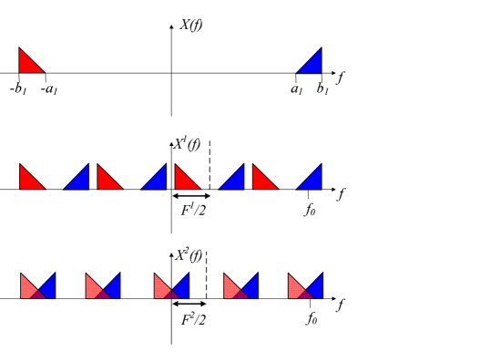
Figure 1: Illustration of the spectrum of a sparse one-band real signal (a), and the spectrum of its samples which are obtained for the sampling rates $F^{1}$ (b) and $F^{2}$ (c). At $f_{0}$, the signal is unaliased at the sampling rate $F^{1}$, but is aliased at the sampling rate $F^{2}$.

One immediate consequence of Eq. 4 is that, up to a phase factor that does not depend on the signal, $\exp[2\pi i(f+nF^{i})\Delta^{i}]$, $X^{i}(f)$ is periodic of period $F^{i}$. It is also clear that, for a real signal $x(t)$, $\overline{X^{i}}(-f)=X^{i}(f)$. Thus, all of the information about $|X^{i}(f)|$ is contained in the interval $[0,F^{i}/2]$. Beside a linear chirp caused by the time offset $\Delta^{i}$ all the information about the phase of $X^{i}(f)$ is also contained in the interval $[0,F^{i}/2]$. We shall refer to this interval $[0,F^{i}/2]$ as the $i$th baseband. The down-conversion of a frequency $f\in[0,F_{\textrm{nyq}}/2]$ to this baseband is represented by the down-conversion function $D^{i}:[0,F_{\textrm{nyq}}/2]\longrightarrow[0,F^{i}/2]$:

$$D^{i}(f)=\min[f\mod F^{i},(F^{i}-f)\mod F^{i}].$$ (5)

In the case of band-limited signal $X(f)$, for a given frequency $f$, all but a finite number of terms in the infinite sum on the right side of Eq. 4 vanish. If the number of non-vanishing terms is greater than one for a given sampling rate $F^{i}$, then the signal is said to be aliased at $f$ when sampled at the rate $F^{i}$. If at a frequency $f$ only a single term in the sum is not equal to zero, the signal $X(f)$ is said to be unaliased at a sampling rate $F^{i}$. Illustration of aliasing can be seen in Fig. 1(c). In the case of sparse signals, $x(t)$ is unaliased at considerable part of it spectral support. The success of an MRS scheme lies in the fact that whereas a signal may be aliased at a frequency $f$ when sampled at a rate $F^{i}$, the same signal may be unaliased at the same frequency $f$ when sampled at a different rate $F^{j}$.

Each support interval $[a,b]$ ($b>a\geq 0$) of the multi-band signal will be referred to as an originating band. According to Eq. 4, sampling at the rate $F^{i}$ down-converts each originating band $[a,b]$ to a single band in the baseband $[\alpha^{i},\beta^{i}]$. We shall refer to the interval $[\alpha^{i},\beta^{i}]$ as a down-converted band.

It is apparent that when a single down-converted band $[\alpha^{i},\beta^{i}]$ is given, it is in general not possible to identify its corresponding originating band. However, it follows easily from Eq. 4 that the corresponding originating band must reside within the set of bands defined by

$$\left\{\left(\bigcup_{m=-\infty}^{\infty}\left[\alpha^{i}+mF^{i},\beta^{i}+mF^{i}\right]\right)\bigcup\left(\bigcup_{m=-\infty}^{\infty}\left[-\beta^{i}+mF^{i},-\alpha^{i}+mF^{i}\right]\right)\right\}\bigcap\left[0,F_{\textrm{nyq}}/2\right],$$ (6)

where $m$ is an integer. The set in Eq. 6 can be represented as a finite number of disjointed closed intervals, which we denote by $[a_{n}^{i},b_{n}^{i}]$. We shall refer to each of these intervals as an up-converted band. For clarity, we denote all down-converted intervals with greek letters superscripted by the sampling frequency and denote all up-converted intervals with latin letters.

In general, the number of possible originating bands is reduced by sampling at more than one rate. For each sampling rate rate $F^{i}$, an originating band $[a,b]$ must reside within the union of the upconverted bands: $[a,b]\in\cup_{n}[a_{n}^{i},b_{n}^{i}]$. Since the union of upconverted bands is different for each sampling rate, sampling at several different rates gives more restrictions over the originating band $[a,b]$. When sampling at $P$ rates, $F^{1},\ldots,F^{p}$, the originating band must reside within $\cap_{i=1}^{P}\cup_{n}[a_{n}^{i},b_{n}^{i}]$.

III Reconstruction Method

In this section we describe an algorithm to reconstruct signals from an MRS scheme. First, we describe an algorithm for reconstructing ideal multi-band signals, as defined above. Then we present modifications to enable a reconstruction of signals that may be contaminated by noise outside of strictly defined bands. While such signals are not exactly multi-band, we still consider them multi-band signals provided that the noise amplitude is considerably lower than the signal amplitude.

The reconstruction is performed sequentially. In the first step sets of intervals in the band $[0,F_{\textrm{nyq}}/2]$ that could be the support of $X(f)$ are identified. These are sets that, when down-converted at each sampling rate $F^{i}$, give energy in intervals in the baseband where significant energy is observed. For each hypothetical support, the algorithm determines the subsets of the support that are unaliased in each channel. According to Eq. 4, for the correct support, the amplitude of each sampled signal spectrum is proportional to the original signal spectrum over the unaliased subset of the support. As a result, for each pair of channels, the amplitudes of the two sampled signal spectra are proportional to one another over the subsets of the hypothetical support which are unaliased in both channels. Thus, we define an objective function that quantifies the consistency between the different channels over mutually unaliased subsets of the support. The algorithm chooses the hypothetical support that maximizes the objective function. The amplitude is reconstructed from the sampled data on the unaliased subsets of the chosen hypothetical support. In the last step, the phase of the spectrum of the originating signal is determined from the unaliased subset of the chosen hypothetical support.

III-A Noiseless signals

In this subsection we assume that all signals are ideal multi-band signals. Although what follows applies to more general signals, we assume that all signals have piece-wise continuous spectrum.

III-A1 Reconstruction of the spectrum amplitude

For each sampled signal $X^{i}(f)$, we consider the indicator function $\mathcal{I}^{i}(f)$ that indicates over which frequency intervals the energy of the sampled signal $X^{i}(f)$ resides. To ignore isolated points discontinuity we define the indicator functions $\mathcal{I}^{i}(f)$ as follows:

$$\mathcal{I}^{i}(f)=\left\{\begin{array}[]{lll}1&&\mathrm{for\;all\;}f\in[0,F_{\textrm{nyq}}/2]\text{\;such that for all\;}\varepsilon>0,\int_{f-\varepsilon}^{f+\varepsilon}|X^{i}(f^{\prime})|^{2}df^{\prime}>0\\ 0&&\mathrm{otherwise}.\end{array}\right.$$

For piece-wise continuous function, it is simple to show that $\mathcal{I}^{i}(f)=1$ on closed intervals.

We define the function $\mathcal{I}(f)$ as follows:

$$\mathcal{I}(f)=\prod_{i=1}^{P}\mathcal{I}^{i}(f),~{}~{}~{}~{}~{}f\in[0,F_{\textrm{nyq}}/2].$$ (7)

Thus, the function $\mathcal{I}(f)$ equals $1$ over the intersection of all the up-converted bands of the $P$ sampled signals. We denote the intervals over which $\mathcal{I}(f)=1$ by $U_{1}\ldots U_{K}$. The Appendix gives sufficient conditions under which each originating band coincides with one of the intervals $U_{1}\ldots U_{K}$. Thus, it remains to determine which of the $K$ intervals coincide with the originating intervals.

For each $k=1,2,\cdots,K$ we consider the indicator function

$$\mathcal{I}_{k}(f)=\left\{\begin{array}[]{lll}1&&\mathrm{if\;}f\in U_{k}\\ 0&&\mathrm{otherwise}.\end{array}\right.$$ (8)

It follows immediately from Eq. 8 that

$$\mathcal{I}(f)=\sum_{k=1}^{K}\mathcal{I}_{k}(f).$$ (9)

To find which sets of $U_{k}$ (or $\mathcal{I}_{k}(f)$) match the originating bands each indicator function $\mathcal{I}_{k}(f)$ is down-converted to the baseband via the formula

$$\mathcal{I}^{i}_{k}(f)=\mathcal{I}_{[0,F^{i}/2]}(f)H\left(\sum_{n=-\infty}^{n=\infty}\mathcal{I}_{k}(f+nF^{i})+\mathcal{I}_{k}(-f+nF^{i})\right).$$ (10)

In Eq. 10 $\mathcal{I}_{[0,F^{i}/2]}(f)$ is the indicator function of the closed interval $[0,F^{i}/2]$:

$$\mathcal{I}_{[0,F^{i}/2]}(f)=\left\{\begin{array}[]{lll}1&\mathrm{if}&f\in[0,F^{i}/2]\\ 0&\mathrm{otherwise}.&\end{array}\right.$$ (11)

$H(f)$ is the Heaviside step function

$$H(f)=\left\{\begin{array}[]{lll}0&\mathrm{if}&f\leq 0\\ 1&\mathrm{if}&f>0.\end{array}\right.$$ (12)

The Heaviside step function in Eq. 10 is used to assure that $\mathcal{I}^{i}_{k}(f)$ is an indicator function. In the case in which the down-conversions of an interval $U_{k}$ are aliased at some frequency $f$ within the baseband the argument of the step function is an integer greater than 1. However, $\mathcal{I}^{i}_{k}(f)=1$. If, for a frequency $f$ in the baseband there is no signal in any of its replicas; i.e., $F(nF^{i}\pm f)=0$ for all $n$, then $H(f)=0$. As a consequence, $\mathcal{I}^{i}_{k}(f)=0$ also. Therefore, the function $\mathcal{I}^{i}_{k}(f)$ is equal to one over the down-conversion of the interval $U_{k}$ corresponding sampling rate $F^{i}$.

We consider the power set of $U$, $\mathcal{P}\{U\}$; i.e., the set of all subsets of $\{U_{1},\cdots,U_{K}\}$. We denote an element of $\mathcal{P}\{U\}$ by $\mathcal{U}=\{U_{k_{1}},\cdots,U_{k_{Q}}\}$ ($0\leq Q\leq K$). A subset $\mathcal{U}\in\mathcal{P}\{U\}$ is deemed to be a support consistent combination if, for each sampling rate $F^{i}$, the down conversion of its intervals matches the down-converted bands of the corresponding sampled signal. In terms of indicator functions, we define for each $\mathcal{U}\in\mathcal{P}\{U\}$ the indicator functions

$$\mathcal{I}^{i}_{\mathcal{U}}(f)=\sum_{U_{k}\in\mathcal{U}}\mathcal{I}^{i}_{k}(f)~{}~{}~{}~{}~{}~{}~{}~{}~{}f\in[0,F^{i}/2].$$ (13)

The function $\mathcal{I}^{i}_{\mathcal{U}}(f)$ is an indicator function for the down-conversion of the intervals of $\mathcal{U}$. Next, we define the objective function

$$E_{1}(\mathcal{U})=\sum_{i=1}^{P}\int_{0}^{F^{i}/2}|\mathcal{I}^{i}_{\mathcal{U}}(f)-\mathcal{I}^{i}(f)|\;\mathrm{d}f.$$ (14)

Support consistent combinations are those $\mathcal{U}$ for which $E_{1}(\mathcal{U})=0$.

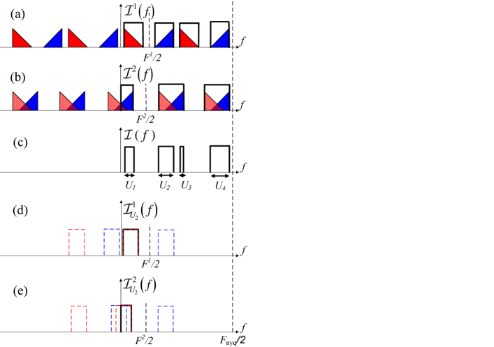
Figure 2: Illustration demonstrating how support-consistency is checked. The input of the algorithm is the sampled signals whose spectra $X^{1}(f)$ and $X^{2}(f)$ are shown Figs. 1 (b) and (c), respectively; their respective indicator functions $\mathcal{I}^{1}(f)$ and $\mathcal{I}^{2}(f)$ are shown in Fig. 2 (a) and (b). Figure 2 (c) shows the indicator function $\mathcal{I}(f)=\mathcal{I}^{1}(f)\mathcal{I}^{2}(f)$. In Figs. 2 (d) and (e), we check whether the subset $\mathcal{U}=\{U_{2}\}\in\mathcal{P}\{U\}$ is support consistent. Figures 2 (d)and (e) show the indicator functions for the down-conversion of $U_{2}$ at rates $F^{1}$ and $F^{2}$: $\mathcal{I}^{1}_{U_{2}}(f)$ and $\mathcal{I}^{2}_{U_{2}}(f)$, respectively. The dashed lines illustrate $U_{2}$, $-U_{2}$ and their down-conversions. It is evident that the functions $\mathcal{I}^{1}(f)$ and $\mathcal{I}^{1}_{U_{2}}(f)$ are not equal. Hence, $\mathcal{U}=\{U_{2}\}$ is not a support-consistent combination.

Figure 2 illustrates our method for the signal shown in Fig. 1. The support of the signal at positive frequencies, shown in Fig. 1, consists of a single interval. Figures 2(a) and 2(b) are graphs of $\mathcal{I}^{1}(f)$ and $\mathcal{I}^{2}(f)$. Figure 2(c) is a graph of $\mathcal{I}(f)$. The function $\mathcal{I}(f)$ is equal to one over four intervals $U_{1},\ldots,U_{4}$. Each combination of these four intervals must be checked for support consistency. In the example illustrated in Fig. 2, we check whether the subset $\mathcal{U}=\{U_{2}\}\in\mathcal{P}\{U\}$ is support consistent. Figures 2 (d) and (e) show the indicator functions for the down-conversion of $U_{2}$ at rates $F^{1}$ and $F^{2}$: $\mathcal{I}^{1}_{U_{2}}(f)$ and $\mathcal{I}^{2}_{U_{2}}(f)$, respectively. The dashed lines illustrate $U_{2}$, $-U_{2}$, and their down-conversions. It is evident that the functions $\mathcal{I}^{1}(f)$ and $\mathcal{I}^{1}_{U_{2}}(f)$ are not equal. Hence, $\mathcal{U}=\{U_{2}\}$ is not a support-consistent combination.

Amongst all support consistent combinations $\mathcal{U}$, it is necessary to identify the one that exactly matches the originating bands. For this purpose, we introduce two additional objective functions. The support consistent combination $\mathcal{U}$ that optimizes these function is deemed to be the correct one.

Amongst support-consistent combinations, amplitude consistent combinations are defined by the amplitudes of the sampled signals at unaliased intervals. Let $\mathcal{U}=\{U_{j_{1}},\cdots,U_{j_{m}}\}$ be a support consistent combination. Denote the union of all intervals in $\bigcup_{n=1}^{m}U_{j_{n}}$ that are unaliased when down-converted at rate $F^{i}$ by $\Sigma^{i}_{\mathcal{U}}\subset\bigcup_{n=1}^{m}U_{j_{n}}$. For the correct choice of $\mathcal{U}$, at a frequency $f$ that is unaliased when sampled at rates $F^{i_{1}}$ and $F^{i_{2}}$ ( $f\in\Sigma_{\mathcal{U}}^{i_{1}}\cap\Sigma_{\mathcal{U}}^{i_{2}}$), the functions $|X^{i_{1}}(f)|/F^{i_{1}}$ and $|X^{i_{2}}(f)|/F^{i_{2}}$ must be equal. Accordingly, we define a second objective function:

$$E_{2}(\mathcal{U})=\sum_{i_{1}\neq i_{2}}\int_{\Sigma_{\mathcal{U}}^{i_{1}}\cap\Sigma_{\mathcal{U}}^{i_{2}}}(|X^{i_{1}}(f)|/F^{i_{1}}-|X^{i_{2}}(f)|/F^{i_{2}})^{2}\;\mathrm{d}f.$$ (15)

For the correct $\mathcal{U}$, the objective function $E_{2}(\mathcal{U})$ must equal zero. A support-consistent combination $\mathcal{U}$ for which $E_{2}(\mathcal{U})=0$ is said to be amplitude consistent.

Unfortunately, there may be more than one amplitude-consistent combination. This is the case, for example, when for all $i_{1}$ and $i_{2}$, $\Sigma^{i_{1}}_{\mathcal{U}}\cap\Sigma^{i_{2}}_{\mathcal{U}}$ is empty. In such cases, the objective function $E_{2}(\mathcal{U})$ cannot be sufficient to identify the correct $\mathcal{U}$. Thus, we introduce a third objective function $E_{3}(\mathcal{U})$. This function favors options in which the integrals in Eq. 15 are calculated over large sets. The third objective function is defined by

$$E_{3}(\mathcal{U})=\sum_{i_{1}\neq i_{2}}\lambda(\Sigma^{i_{1}}_{\mathcal{U}}\cap\Sigma_{\mathcal{U}}^{i_{2}}),$$ (16)

where $\lambda(\Sigma^{i_{1}}_{\mathcal{U}}\cap\Sigma_{\mathcal{U}}^{i_{2}})$ is the Lebesgue measure of $\Sigma^{i_{1}}_{\mathcal{U}}\cap\Sigma_{\mathcal{U}}^{i_{2}}$. The amplitude-consistent combination that maximizes $E_{3}(\mathcal{U})$ is deemed to be the correct one. In the rare case that $E_{3}(\mathcal{U})$ is maximized by more than one amplitude-consistent combination, the outcome of the algorithm is not determined.

After the optimal $\mathcal{U}=\{U_{j_{1}},\cdots,U_{j_{m}}\}$ is chosen, the amplitude of the signal is reconstructed from the samples. We define the function $r(f)$ as the number of sampled signals which are unaliased at the frequency $f$: $r(f)=\sum_{i=1}^{P}\mathcal{I}_{\Sigma^{i}_{\mathcal{U}}}(f)$, where $\mathcal{I}_{\Sigma^{i}_{\mathcal{U}}}(f)$ is the indicator function of the interval ${\Sigma^{i}_{\mathcal{U}}}$, defined similarly to Eq. 11. For each $f$ within the detected originating bands, i.e. $f\in\bigcup_{n=1}^{m}U_{j_{n}}$, if $r(f)>0$, we reconstruct the corresponding amplitude of the spectrum at $f$ from the sampled signals by

$$X_{\mathcal{U}}(f)=\frac{1}{r(f)}\sum_{i=1}^{P}\frac{|X^{i}(f)|\mathcal{I}_{\Sigma^{i}_{\mathcal{U}}}(f)}{F^{i_{n}}}.$$ (17)

In words, for each frequency $f$ that is unaliased in at least one channel, the signal amplitude is averaged over all the channels that are not aliased at $f$. For all other frequencies, notably those that alias in all sampling channels, $X_{\mathcal{U}}(f)$ is set to equal zero.

III-A2 Reconstruction of the spectrum phase

The spectrum of a signal can be expressed as $X(f)=|X(f)|\exp\{j\arg[X(f)]\}$. In the previous section we described how to reconstruct the amplitude $|X(f)|$ from the signal’s sampled data. In this section we describe a method of reconstructing the phase $\arg[X(f)]$. If the time offsets $\Delta^{i}$ of Eq. 4 were known a priori, reconstructing the phase would be trivial. The reconstruction in this case could be performed by using a variant of Eq. 17 with $|X^{i_{n}}(f)|$ replaced by $X^{i_{n}}(f)\exp(-2\pi f\Delta^{i_{n}})$. This would yield a full reconstruction of the signal (phase and amplitude). However, because of the lack of synchronization between the channels, the time offsets $\Delta^{i}$ are not known a priori. Consequently, it is more difficult to reconstruct the phase. After identifying the signal bands, we can calculate the differences $\Delta^{i_{1}}-\Delta^{i_{2}}$ between two different time offsets. This is sufficient to enable the reconstruction of the phase of the signal spectrum up to a single linear phase factor.

The difference between two time offsets $\Delta^{i_{1}}$ and $\Delta^{i_{2}}$ can be calculated directly in the case that $\Sigma_{\mathcal{U}}^{i_{1}}\cap\Sigma_{\mathcal{U}}^{i_{2}}$ contains at least one finite interval. In this interval the phase of $X^{i_{1}}(f)/X^{i_{2}}(f)$ satisfies the following equation:

$$\arg[X^{i_{1}}(f)/X^{i_{2}}(f)]=2\pi f(\Delta^{i_{1}}-\Delta^{i_{2}})+2\pi k,~{}~{}~{}~{}~{}~{}\text{for some integer}~{}k$$ (18)

The left side of Eq. 18 is determined by the sampled data. By performing a linear fit we calculate the difference between the two offsets $\Delta^{i_{1}}$ and $\Delta^{i_{2}}$. We do this for all pairs of offsets for which $\Sigma_{\mathcal{U}}^{i_{1}}\cap\Sigma_{\mathcal{U}}^{i_{2}}$ contains at least one finite interval.

There may exist cases in which there exist $i_{1}$ and $i_{2}$ such that $\Sigma_{\mathcal{U}}^{i_{1}}\cap\Sigma_{\mathcal{U}}^{i_{2}}$ does not contain one finite interval but for which $\Delta^{i_{1}}-\Delta^{i_{2}}$ can still be calculated. For example, in the case of three offsets $\Delta^{i_{1}}$, $\Delta^{i_{2}}$ and $\Delta^{i_{3}}$, if one can calculate $(\Delta^{i_{1}}-\Delta^{i_{2}})$ and $(\Delta^{i_{2}}-\Delta^{i_{3}})$, then $(\Delta^{i_{1}}-\Delta^{i_{3}})$ can also be calculated by simple algebra. If there exist ${i_{n}},\ldots{i_{m}}$, such that for each ${n}\leq k\leq{m-1}$, $\Sigma_{\mathcal{U}}^{i_{k}}\cap\Sigma_{\mathcal{U}}^{i_{k+1}}$ contains at least one finite interval, then we say that $i_{n}$ and ${i_{m}}$ are phase connected and denote this by ${i_{n}}\sim{i_{m}}$. If $i\sim j$, then difference between the two offsets $\Delta^{j}-\Delta^{i}$ can be calculated. In the case $\Sigma_{\mathcal{U}}^{i}$ does not contain any finite intervals, we define $\Delta^{i}\sim\Delta^{i}$. It is clear that $\sim$ is an equivalence relation [10] and thus partitions the $\Delta^{i}$ into equivalence classes.

For each $\Delta^{i_{1}}$ and $\Delta^{i_{2}}$ in the same class, one can calculate their difference. One can obtain a full reconstruction of the phase if there exists one class $\mathcal{C}$ such that each originating frequency is unaliased in at least one channel belonging to $\mathcal{C}$; i.e, there exist a class $\mathcal{C}=\Delta^{i_{n}}\ldots\Delta^{i_{m}}$, such that $\bigcup_{k=n}^{m}\Sigma_{\mathcal{U}}^{i_{k}}=\bigcup_{k=1}^{Q}U_{j_{k}}$, where $\mathcal{U}=\{U_{j_{1}},\cdots,U_{j_{Q}}\}$.

III-B Physical signals

To sample realistic signals (i.e., not strictly multi-band and in the presence of noise), the algorithm needs to be adjusted. In this subsection we describe adjustments to our algorithm to overcome the noise. The algorithm requires five new parameters. In section 5, we give examples of reconstructing signals contaminated by strong noise. In those examples, the success of the reconstruction does not depend on the exact choice of the five parameters.

In the presence of noise, the definition of the support of the sampled signals must be adjusted. First, a small $\xi$ is chosen. Then, a small positive threshold value $T$ is chosen. The indicator function $\mathcal{I}^{i}(f)$ is then redefined as follows:

$$\mathcal{I}^{i}(f)=\left\{\begin{array}[]{lll}1&&\mathrm{if\;}f\in[0,F_{\textrm{nyq}}/2]\;\mathrm{and}\;\frac{1}{2\xi}\int_{f-\xi}^{f+\xi}|X_{\alpha}(f^{\prime})|df^{\prime}>T\\ 0&&\mathrm{otherwise}.\end{array}\right.$$ (19)

The choice of the threshold $T$ depends on the average noise level.

When reconstructing physical signals, it is not reasonable to expect $E_{1}(\mathcal{U})$ to equal 0 for any combination $\mathcal{U}$. An initial adjustment is to require that $E_{1}(\mathcal{U})<b$ for some positive $b$. The shortcoming of this condition is that the threshold $b$ does not depend on the signal. To make the threshold to depend on the signal in a simple way, we introduce the following condition:

$$E_{1}(\mathcal{U})<a\min_{\mathcal{U}}\left[E_{1}(\mathcal{U})\right]+b$$ (20)

where $a\geq 1$ is a chosen parameter. The parameters $a$ and $b$ control the tradeoff between the chance of success and runtime. If $a$ and $b$ are too small, the correct subset $\mathcal{U}$ may not be included in the set of support constituent combinations. On the other hand, if $a$ and $b$ are too large, then the number of support-consistent combinations may be large. This results in a slow run time.

Finally, we make two modifications to the objective function $E_{3}(\mathcal{U})$. We replace the length of the mutually unaliased intervals by a weighted energy of the sampled signals in these interval. The objective function $E_{3}(\mathcal{U})$ is replaced with $\widehat{E}_{3}$:

$$\widehat{E}_{3}(\mathcal{U})=\sum_{i_{1}\neq i_{2}}\int_{0}^{F_{\textrm{nyq}}/2}\left|\frac{X^{i_{1}}(f)}{F^{i_{1}}}\right|^{2}{W}_{i_{1},i_{2}}(f,\mathcal{U})\;\mathrm{d}f,$$ (21)

where ${W}_{i_{1},i_{2}}(f,\mathcal{U})$ is a weight function. The weight function favors combinations in which the sampled signals are similar in mutually unaliased internals and is defined in the following.

We first note that for each two channels $i_{1}$ and $i_{2}$, the intersection of their non-aliased supports ($\Sigma^{i_{1}}_{\mathcal{U}}\cap\Sigma_{\mathcal{U}}^{i_{2}}$) is a union of a finite number of disjoint intervals $V_{1}^{i_{1},i_{2}},\cdots V_{R}^{i_{1},i_{2}}$. We define

$$\mu^{k}_{i_{1},i_{2}}(\mathcal{U})=\frac{\int_{V_{k}^{i_{1},i_{2}}}|\;|X^{i_{1}}(f)|/F^{i_{1}}-|X^{i_{2}}(f)|/F^{i_{2}}\;|\;\mathrm{d}f}{\int_{V_{k}^{i_{1},i_{2}}}|\;|X^{i_{1}}(f)|+|X^{i_{2}}(f)|\;|\;\mathrm{d}f}.$$ (22)

Finally, we define the weight function:

$$W_{i_{1},i_{2}}(f)=\sum_{k}\exp[-\rho{\mu}^{k}_{i_{1},i_{2}}(\mathcal{U})]{\mathcal{I}}_{V_{k}^{i_{1},i_{2}}}(f),$$ (23)

where $\rho$ is a chosen positive constant and $\mathcal{I}_{V_{k}^{i_{1},i_{2}}}(f)$ is the indicator function of the interval $V_{k}^{i_{1},i_{2}}$. The parameter $\rho$ is chosen according to an assumed signal to noise ratio (SNR). When the SNR is lower, in order to accept higher errors $\rho$ is chosen to be smaller. In the case of a noiseless signal and an amplitude-consistent ${\mathcal{U}}$, each $\mu^{k}_{i_{1},i_{2}}$ vanishes. Therefore, in this case, each element in the sum on the right-hand side of Eq. 21 gives the energy of the signal over $\Sigma^{i_{1}}_{\mathcal{U}}\cap\Sigma_{\mathcal{U}}^{i_{2}}$. In all other cases, the energy in each interval $V_{k}^{i_{1},i_{2}}$ is weighted according to the relative error between $X^{i_{1}}(f)$ and $X^{i_{2}}(f)$ over $V_{k}^{i_{1},i_{2}}$.

Since in the case of noisy signals, neither $E_{1}(\mathcal{U})$ nor $E_{2}(\mathcal{U})$ vanishes for the combination which corresponds to the originating bands, both $E_{1}(\mathcal{U})$ and $E_{2}(\mathcal{U})$ should be considered in the final step of choosing the best combinations. Accordingly, we define the following objective function $E_{\text{tot}}(\mathcal{U})$:

$$E_{\text{tot}}(\mathcal{U})=-\frac{E_{1}(\mathcal{U})}{\min_{\mathcal{U}}\left\{E_{1}(\mathcal{U})\right\}}-\frac{E_{2}(\mathcal{U})}{\min_{\mathcal{U}}\left\{E_{2}(\mathcal{U})\right\}}+\frac{\widehat{E}_{3}(\mathcal{U})}{\min_{\mathcal{U}}\left\{\widehat{E}_{3}(\mathcal{U})\right\}}$$ (24)

for all $\mathcal{U}$ such that ${\min_{\mathcal{U}}\left\{E_{1}(\mathcal{U})\right\}},{\min_{\mathcal{U}}\left\{E_{2}(\mathcal{U})\right\}},{\min_{\mathcal{U}}\left\{E_{3}(\mathcal{U})\right\}}\neq 0$. Amongst all such combinations that also satisfy Eq. 20, the one that gives the maximum value of $E_{\text{tot}}(\mathcal{U})$ is deemed to be correct. In cases in which either $\min_{\mathcal{U}}\left\{E_{1}(\mathcal{U})\right\}$, $\min_{\mathcal{U}}\left\{E_{2}(\mathcal{U})\right\}$ or $\min_{\mathcal{U}}\left\{E_{3}(\mathcal{U})\right\}$ equals zero for a certain combination $\mathcal{U}$, the maximum of $\widehat{E}_{3}(\mathcal{U})$ is chosen as the solution.

To reconstruct the phase, the only change made is in how the difference between the offsets is calculated. Equation 18 holds for all the disjoint intervals $V_{k}^{i_{1},i_{2}}\in\Sigma_{\mathcal{U}}^{i_{1}}\cap\Sigma_{\mathcal{U}}^{i_{2}}$. Accordingly, we perform the linear fit for each intervals, and obtain a certain value for $\Delta^{i_{1}}-\Delta^{i_{2}}$. Each value is weighted by the length of its respective $V_{k}^{i_{1},i_{2}}$. These weighted values are averaged. The result is an estimate for $\Delta^{i_{1}}-\Delta^{i_{2}}$. This averaging procedure may increase the accuracy in the estimate of $\Delta^{i_{1}}-\Delta^{i_{2}}$.

IV Complexity considerations

In this section we discuss considerations used to reduce the computational complexity of our algorithm. Choosing a subset $\mathcal{U}\in\mathcal{P}\{U\}$ involves calculating three objective functions. We explain why eliminating possibilities through the use of $E_{1}(\mathcal{U})$ alone can significantly reduce runtime.

In the first step of the algorithm, we find support consistent combinations by calculating the objective function $E_{1}(\mathcal{U})$ for elements in $\mathcal{P}\{U\}$. Assuming the largest element in $\mathcal{P}\{U\}$ contains $K$ intervals, and that the signal is composed of up to $N$ bands in $[0,F_{\textrm{nyq}}/2]$, the number of elements in $\mathcal{P}\{U\}$ that one needs to check is equal to

$$\sum_{n=1}^{N}\left(\begin{array}[]{cc}K\\ n\end{array}\right).$$ (25)

In the case $N\approx K$, the complexity is approximately $O(2^{N})$. When $N/K\ll 1$, the last term in Eq. 25 number of options to be checked is approximately equal to $O(K^{N}/N!)$.

The complexity of checking a single option out of $\mathcal{P}\{U\}$ for support consistency (Eq. 14) is $O(1)$ and it does not depend on the number of points used to discretize the spectrum. By contrast, the complexity of checking such an option for amplitude consistency (Eqs. 15 and 16) is of the order of the number of points used to represent the spectrum. This is a major reason for using the support-consistency criterion to narrow down the number of options needed to be checked for amplitude consistency. The amplitude consistency is calculated only for support-consistent options, which are in general much fewer than what is prescribed by Eq. 25.

V Numerical Results

This section describes results of our numerical simulations. The simulations were carried out in the two cases considered in the previous sections: i) ideal multi-band signals and ii) noisy signals. In all our examples, the number of channels $P$ was set equal to three, $P=3$.

In all our simulations, the number the bands in $[0,F_{\textrm{nyq}}/2]$ equals $N$, where $N\leq 4$. Unless stated otherwise the band number refers to the number of bands in the non negative frequency region $[0,F_{\textrm{nyq}}/2]$. Using the notations in Eq. 2, each signal in each band is given by

$$S_{n}(f)=\left\{\begin{array}[]{lll}A_{n}\cos[\pi(f-f_{n})/B_{n}]&&\mathrm{if\;}2|f-f_{m}|/B_{n}<1\\ 0&&\mathrm{otherwise},\end{array}\right.$$ (26)

where $B_{n}$ is the spectral width of the $n$th band, $f_{n}$ is its central frequency, and $A_{n}$ is the maximum amplitude. The total spectral measure of the signal support equals $\Sigma_{x}=2\sum_{n=1}^{N}B_{n}$, and the minimal sampling rate is equal to $2\Sigma_{x}$ [6], twice the Landau rate. In each simulation, all the bands had the same width, i.e. $B_{n}=\Sigma_{x}/(2N)$. The amplitudes $A_{n}$ were chosen independently from a uniform distribution on $[1,1.2]$. The central frequencies $f_{n}$ were also chosen independently from a uniform distribution on the region $[0,F_{\textrm{nyq}}/2]$. We eliminated cases in which there was an overlap between any two different bands. The time offsets, $\Delta^{i}$ were chosen independently from a uniform distribution on $[0,1/B_{n}]$.

In each of the simulations, we set $B=800$ MHz and $40\leq F_{\textrm{nyq}}\leq 76$ GHz. This choice of parameters is consistent with previous optical sampling experiments [1]. The sampling rates were chosen as $F^{1}=3.8F_{0}$, $F^{2}=4F_{0}$, and $F^{3}=4.2F_{0}$, where the value $F_{0}$ varied between simulations. These sampling rates were chosen such that, for each pair of sampling rates ($F^{i}$, $F^{j}$), the functions $\mathcal{I}^{i}(f),~{}\mathcal{I}^{j}(f)$ do not have a common multiple smaller than $F_{\textrm{nyq}}$. This condition is satisfied for all $F_{0}>F_{\textrm{nyq}}/76$.

To obtain an exact reconstruction, the resolution in which the spectrum is represented $\Delta f$ should be such that the discretization of the originating baseband downconverts exactly to the discretization grid in each baseband. This condition is satisfied when $F^{i}/\Delta f$ ($i=1,2,3$) is an integer. In our examples, we used a spectral resolution $\Delta f=0.8$MHz for all the channels.

The use of the same spectral resolution for all channels is not only convenient for implementation of our algorithm, but it also compatible with the operation of the sampling system used in our experiments [1]. In the implementation of the sampling system, an optical system performs the down conversion of the signal by multiplying it by a train of short optical pulses. In each channel a different repetition rate of the optical pulse train is used. The sampled signal in each channel is then converted into an electronic signal and passed through a low-pass filter which rejects all frequencies outside the baseband. The $P$ filtered sampled signals have a limited bandwidth. These signals are sampled once more, this time at a constant rate, using $P$ electronic analog to digital converters. The use of the optical system allows the use of electronic analog to digital converters whose bandwidth is significantly lower than the bandwidth of the multi-band signal [1]. Because the signals at the basebands are sampled with the same time resolution and have the same number of samples, their spectra, which are obtained using the Fast Fourier Transform, have the same spectral resolution.

In the first set of simulations we increased the signal bandwidth, without changing the sampling rates. We used two performance criteria: correct detection of the originating bands and exact reconstruction of the signal. As to the first criterion, we required only that the spectral support of the signal be detected without an error. As to the second criterion, we required that the signal spectrum (phase and amplitude) be fully and exactly reconstructed without any error. Because the second criterion concerns exact reconstructions, in the case that the algorithm failed to reconstruct the signal at even a single frequency, it was considered to have failed the second criterion.

We chose $F_{0}=1$ GHz. This corresponds to a total sampling rate $F_{\text{tot}}=F^{1}+F^{2}+F^{3}$ which equals 15 times the Landau rate (7.5 the minimum possible rate). The statistics were obtained by averaging over 1000 runs. Figures 3 (a) and (b) show the results for signals with 3 and 4 positive bands, respectively, as a function of the Nyquist rate. In Fig. 3 (a), the percentage of a correct band detection is shown by the squares, whereas the full reconstruction percentage is shown by circles. The open circles and squares represent the results obtained when the maximum number of bands assumed by the algorithm was 3, and the dark circles and squares represent the cases in which the maximum assumed band number was equal to 4. Figure 3 (b) shows the band-detection percentage (solid curve) and reconstruction percentages (dashed curve) in the case that both the maximum number of originating and assumed bands is 4. The figures show that both the success percentages were high and were not significantly dependent on the Nyquist rate of the signal or on the number of assumed bands.

$\begin{array}[]{c@{\hspace{1in}}c}\lx@intercol\hfil\lx@intercol&\lx@intercol\hfil\lx@intercol\\ \hbox{\includegraphics[angle={-90},width=256.0748pt]{ideal_nyq34.eps}}\hfil\hskip 72.26999pt&\hbox{\includegraphics[angle={-90},width=256.0748pt]{ideal_nyq44.eps}}\\ \vspace{-1cm}\mbox{\bf(a)}\hfil\hskip 72.26999pt&\mbox{\bf(b)}\end{array}$

Figure 3: Success percentage for the first set of simulations with $F_{0}=1$ GHz as a function of Nyquist rate. In Fig. 3 (a), the percentage of a correct band detection is shown by the squares. The full reconstruction percentage is shown by circles. The open circles and squares represent the results obtained when the assumed maximum number of positive bands equals 3. The dark circles and squares represent the cases in which the maximum assumed positive band number equals 4. Figure 3 (b) shows the band-detection percentage (solid curve) and reconstruction percentages (dashed curve) in the case that both the maximum number of originating and assumed positive bands equals 4.

Figure 4: The run time for the second set of simulations as a function of the Nyquist rate. The results in the case of 4 input positive bands with assumed number of positive bands equals 4 is shown in the solid curve. The results in the case of 3 input positive bands is shown with the dotted curve in the case of 3 assumed positive bands and with the dashed curve in the case of 4 assumed positive bands.

Figure 4 shows the average run time as a function of the Nyquist rate. The results in the case of 4 input bands in which the assumed maximum number of bands is 4 is shown in the solid curve. The results in the case of 3 input bands is shown with the dotted curve in the case of 3 assumed bands and with the dashed curve in the case of 4 assumed bands. The results show that while an increase in the Nyquist rate does not significantly affect the reconstruction statistics, it results in an increase in run time.

In the second set of simulations, we measured the performance of our algorithm as a function of $F_{0}$. The Nyquist rate used in the simulation was $F_{\textrm{nyq}}=40$ GHz. For each choice of $F_{0}$, the statistics were obtained by averaging over 500 runs. The results did not change significantly when the averaging was performed over 1000 runs. The simulation was run for the same number of originating bands and assumed bands as in the first set of simulations. Figures 5 (a) and (b) show the success percentages for signals with 3 and 4 bands, respectively, and Fig. 6 shows the average run time. The two success percentages and run time are shown as a function of the total sampling rate $F_{\text{tot}}$ divided by the Landau rate, $F_{\text{Landau}}=800$ MHz. The symbols used in Figs. 5 (a) and (b) and Fig. 6 correspond to those used in Figs. 3 (a) and (b) and Fig. 4 respectively.

$\begin{array}[]{c@{\hspace{1in}}c}\lx@intercol\hfil\lx@intercol&\lx@intercol\hfil\lx@intercol\\ \hbox{\includegraphics[width=256.0748pt]{ideal_freq34.eps}}\hfil\hskip 72.26999pt&\hbox{\includegraphics[width=256.0748pt]{ideal_freq44.eps}}\\ \vspace{-1cm}\mbox{\bf(a)}\hfil\hskip 72.26999pt&\mbox{\bf(b)}\end{array}$

Figure 5: Success percentage for the first set of simulations as a function of the sum of the sampling rates divided by the Landau rate. As in Fig. 3, in Fig. 5 (a), the percentage of a correct band detection is shown by the squares. The full reconstruction percentage is shown by circles. The open circles and squares represent the results obtained when the assumed maximum number of positive bands equals 3. The dark circles and squares represent the cases in which the maximum assumed positive band number equals 4. Figure 5 (b) shows the band-detection percentage (solid curve) and reconstruction percentages (dashed curve) in the case that both the maximum number of originating and assumed positive bands equals 4.

The results shown in Figs. 5 (a) and (b) demonstrate that, in all the cases that we checked, the average percentage of successful band detection was over 99.5% for sampling frequencies above 8 times the Landau rate. The reconstruction percentages were lower than these band-detection percentages and were also much more affected by the sampling rate and by the number of originating bands. As expected, the run time increases dramatically with reduction of the sampling rate and also increases with the assumed maximum number of bands. We ran similar simulations with different numbers of originating bands and different numbers of assumed bands. The trends were similar.

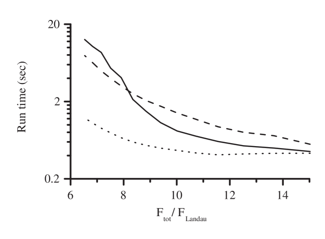
Figure 6: The run time for the first set of simulations as a function of the sum of the sampling rates divided by the Landau rate in the cases of signals with 4 and 3 positive bands. The results in the case of 4 input positive bands with assumed number of positive bands equals 4 is shown in the solid curve. The results in the case of 3 input positive bands is shown with the dotted curve in the case of 3 assumed positive bands and with the dashed curve in the case of 4 assumed positive bands.

In the final set of simulations, the signals are noisy. We added to the originating signal white Gaussian noise in the band $[-F_{\textrm{nyq}}/2,F_{\textrm{nyq}}/2]$, where $F_{\textrm{nyq}}=40$ GHz. We denote by $\sigma$ the standard deviation of the Gaussian noise in the pre-sampled signal. Upon sampling the signal at rate $F^{i}$, the standard deviation of the noise increases to $\sigma^{i}=\sigma\sqrt{\lceil F_{\textrm{nyq}}/F^{i}\rceil}$ owing to aliasing of the noise, where $\lceil x\rceil$ equals the smallest integer greater or equal to $x$.

Figure 7: Success percentage for the third set of simulations with $F_{0}=1$ GHz and $F_{\textrm{nyq}}=20$ GHz as a function of standard deviation $\sigma$ of the added noise. The figure shows the band-detection percentage (solid curve) and reconstruction percentages (dashed curve) in the case that both the maximum number of originating and assumed positive bands equals 4.

In the this set of simulations, we reconstructed signals with different noise levels added. We chose $\xi=6$ MHz. The threshold was chosen to be $T=2\max_{i}(\sigma^{i})$. Accordingly, the parameter $\rho$ in Eq. 23 was chosen to be $\rho=\max_{i}(\sigma^{i})$. The other parameters used in the simulation were $a=2$ and $b=16$ MHz. Because the signals were not ideal, an exact reconstruction was not possible and the definitions of an accurate band detection and accurate reconstruction needed to be changed. A band detection was deemed accurate if the originating bands approximately matched the reconstructed bands. A signal reconstruction was deemed accurate if the signal’s originating bands were detected accurately and if each reconstructed band $X_{\mathcal{U}}(f)$ satisfied

$$\int_{B_{m}}|X_{\mathcal{U}}(f)-X(f)|<\max_{i}(\sigma^{i})B_{m}.$$ (27)

Here $X(f)$ is the noiseless signal and the integration is performed over only the detected band. In a correct reconstruction, it is expected that the average reconstruction error is lower than the standard deviation of the noise in the noisiest channel, i.e. the channel at the lowest sampling rate. We chose the same sampling rates as those chosen in the second set of simulations. For these rates: $\max_{i}(\sigma^{i})=3.3\sigma$.

The detection percentages and reconstruction percentages are shown in Fig. 7. The figure clearly shows that high percentages are obtained even in the case of low signal to noise ratio. We repeated this last
set of simulations using Gaussian signals instead of the signals of Eq. 26. We found that results are not sensitive to the specific choice of signal type.

VI Conclusion

Typical undersampling schemes are PNS schemes. In such schemes samples are taken from several channels at the same low rate. These schemes have many drawbacks. In this paper we propose a new scheme for reconstructing multi-band signals under the constraint of a small number of sampling channels. We have developed an MRS scheme; a scheme in which each channel samples at a different rate. We have demonstrated that sampling with our MRS scheme can overcome many of the difficulties inherent in PNS schemes and can effectively reconstruct signals from undersampled data. For a typical sparse multi-band signal, our MRS scheme has the advantage over PNS schemes because in almost all cases, the signal spectrum is unaliased in at least one of the channels. This is in contrast to PNS schemes. With PNS schemes an alias in one channel is equivalent to an alias in all channels.

Our MRS scheme uses a smaller number of sampling channels than do PNS schemes. We also choose to sample at a higher sampling rate than PNS schemes use in attaining the theoretical minimum overall sampling rate required for a perfect reconstruction. The use of higher rates has an inherent advantage in that it increases the sampled signal to noise ratio. Our MRS scheme also does not require the solving of poorly conditioned linear equations that PNS schemes must solve. This eliminates one source of lack of robustness of PNS schemes. Our simulations indicate that our MRS scheme, using a small number of sampling channels (3 in our simulations) is robust both to different signal types and to relatively noisy signals.

Our reconstruction scheme does not require the synchronization of different sampling channels. This significantly reduces the complexity of the sampling hardware. Moreover, asynchronous sampling does not require very low jitter between the sampling time at different channels as is required in PNS schemes. Our reconstruction scheme resolves aliasing in almost all cases but not all. In rare cases, reconstruction of the originating signal fails owing to aliasing. One of the methods to resolve aliasing is to synchronize the sampling in all the channels. With such synchronization, aliasing can be resolved by inverting a matrix similarly to as is done in PNS schemes. However, such an approach requires both much more complex hardware and a larger number of sampling channels that sample with a very low jitter. Moreover, in case of signals that are aliased simultaneously in all channels, the noise in the reconstructed signal is expected to be much stronger than the noise in the original signal.

Future work should focus on testing our algorithm’s ability to reconstruct experimental data. Optical systems for performing experiments are currently in existence.

VII Appendix

In section 3.A.1 we have denoted the intervals over which the indicator function $\mathcal{I}(f)=1$ by $U_{1}\ldots U_{K}$. In this appendix we give a sufficient and necessary conditions under which the spectral support of a signal coincides with a subset $\mathcal{U}$ of $\{U_{1},\ldots U_{K}\}$ and under which the function $E_{1}(\mathcal{U})$ (Eq. 14) is equal to zero. Although it applies for more general cases, we assume that the function $X(f)$ is piecewise continuous.

The conditions are as follows:

1. For each frequency $f_{0}$ which fulfills $\int_{f_{0}-\varepsilon}^{f_{0}+\varepsilon}|X(f)|^{2}df>0$ for all $\varepsilon>0$, we obtain that
   $\int_{f_{0}-\varepsilon}^{f_{0}+\varepsilon}|X^{i}(f)|^{2}df>0$ for all $\varepsilon>0$ and $1\leq i\leq P$.

2. For each originating band with support $[a,b]$, there exists an interval $[a-\varepsilon,a+\varepsilon]$, ($\varepsilon\neq 0)$ whose down-converted band does not overlap any other down-converted band in at least one of the sampled signals. Similarly, for each originating band with support $[a,b]$, there exists an interval $[b-\varepsilon,b+\varepsilon]$, whose down-converted band does not overlap any other down-converted band in at least one of the sampled signals.

Condition 1 assures that originating bands are contained within $\cup_{i=1}^{K}U_{i}$. Condition 2 guarantees that the originating coincide exactly with a subset of $\mathcal{P}\{U\}$. It is obvious that when the conditions are satisfied, $E_{1}(\mathcal{U})=0$.

The first condition excludes cases in which the down-converted bands cancel each other’s energy over a certain interval due to destructive interference. When the condition is fulfilled, for each frequency $f_{0}$ within the originating bands, we obtain $\mathcal{I}(f_{0})=1$. Thus, each originating band $[a,b]$ is contained within one of the intervals that make up the support of $\mathcal{I}(f)$. Mathematically, for each $[a,b]$, there exist $U_{k}$, such that $[a,b]\subseteq U_{k}$.

The second conditions assures us that for each originating band $[a,b]$, the intervals $[a-\varepsilon,a]$ and $[b,b+\varepsilon]$ are not contained within any of the $U_{k}$ for all values of $\varepsilon$. Consequentially, if $[a,b]\subseteq U_{k}$, then $[a,b]=U_{k}$. When the two conditions are fulfilled, we obtain that there exist a set of intervals $\mathcal{U}$, which matches the originating bands, and for which $E_{1}(\mathcal{U})=0$

References

- [1] A. Zeitouny, A. Feldser, and M. Horowitz, “Optical sampling of narrowband microwave signals using pulses generated by electroabsorption modulators,” Opt. Comm., 256, 248-255 (2005).
- [2] H. Landau, “Necessary density conditions for sampling and interpolation of certain entire functions,” Acta Math., 117, 37 -52 (1967).
- [3] A. Kohlenberg, “Exact Interpolation of Band-limited Functions,” J. Appl. Phys., 24, 1432–1436 (1953).
- [4] R. Venkantaramani and Y. Bresler, “Optimal sub-nyquist nonuniform sampling and reconstruction for multiband signals,” IEEE Trans. Signal Process., 49, 2301–2313 (2001).
- [5] Y. M. Lu and M. N. Do, “A Theory for Sampling Signals from a union of Subspaces,” IEEE Trans. Signal Process., to be published.
- [6] M. Mishali and Y. Eldar, “Blind multi-band signal recostruction: compressed sensing for analog signals,” arXiv:0709.1563 (September 2007).
- [7] P. Feng and Y. Bresler, “Spectrum-blind minimum-rate sampling and reconstruction of multiband signals,” in Proc. IEEE Int. Conf. ASSP, Atlanta, GA, IEEE, MAY 1996.
- [8] Y. P. Lin and P. P. Vaidyanathan, “Periodically uniform sampling of bandpass signals,” IEEE Trans. Circuits Sys., 45, 340–351 (1998).
- [9] C. Herley and W. Wong, “Minimum rate sampling and reconstruction of signals with arbitrary frequency support, IEEE Trans. Inform. Theory, 45, 1555–1564 (1999).
- [10] I. Stewart and D. Tall, The Foundations of Mathematics. Oxford, England: Oxford University Press, 1977.