MANY-BODY THEORY OF THE
ELECTROWEAK NUCLEAR RESPONSE

Abstract

After a brief review of the theoretical description of nuclei based on nonrelativistic many-body theory and realistic hamiltonians, these lectures focus on its application to the analysis of the electroweak response. Special emphasis is given to electron-nucleus scattering, whose experimental study has provided a wealth of information on nuclear structure and dynamics, exposing the limitations of the shell model. The extension of the formalism to the case of neutrino-nucleus interactions, whose quantitative understanding is required to reduce the systematic uncertainty of neutrino oscillation experiments, is also discussed.

1 Introduction

Over the past four decades, electron scattering has provided a wealth of information on nuclear structure and dynamics. Form factors and charge distributions have been extracted from elastic scattering data, while inelastic measurements have allowed for a systematic study of the dynamic response over a broad range of momentum and energy transfer.[1] In addition, with the advent of the last generation of continuous beam accelerators, a number of exclusive processes have been analyzed with unprecedented precision (for recent reviews, see, e.g. Ref.[2]).

In electron scattering experiments the nucleus il mostly seen as a target. Studying its interactions with the probe, whose properties are completely specified, one obtains information on the unknown features of its internal structure.

The emerging picture clearly shows that the nuclear shell model fails to provide a fully quantitative description of the existing data. More realistic many body approaches, in which correlation effetcs are explicitely taken into account, appear to be needed to explain electron scattering observables.

In neutrino oscillation experiments, on the other hand, nuclear interactions are exploited to detect the beam particles, whose kinematics is largely unknown. Using the nucleus as a detector obviously requires that its response to neutrino interactions be under control. Fulfillment of this prerequisite is in fact critical to keep the systematic uncertainty associated with the reconstruction of the neutrino kinematics to an acceptable level.[3]

These lectures are aimed at providing an introduction to nuclear many-body theory and its application to the calculation of the electron- and neutrino-nucleus cross section. Section 2 contains a short overview of the underlying dynamical model and formalism. For pedagogical purposes, the nuclear response is first analyzed in the case of a scalar probe in Section 3, while the generalization to electron and charged current neutrino interactions is discussed in Sections 4 and 5, respectively. Finally, Section 6 is devoted to a summary of the main results.

2 Non relativistic Nuclear Many-Body Theory

In nuclear many-body theory (NMBT) the nucleus is viewed as a collection of $A$ pointlike protons and neutrons, whose dynamics are described by the nonrelativistic hamiltonian

$$H=\sum_{i}\frac{{\bf p}_{i}^{2}}{2m}+\sum_{j>i}v_{ij}+\sum_{k>j>i}V_{ijk}\ ,$$ (1)

where ${\bf p}_{i}$ and $m$ denote the momentum of the $i$-th nucleon and the nucleon mass, respectively. The two body potential $v_{ij}$ is determined by fitting deuteron properties and $\sim$ 4000 precisely measured nucleon-nucleon (NN) scattering phase shitfs.[4] It turns out to be strongly spin-isospin dependent and non central, and reduces to the Yukawa one pion exchange potential at large separation distance. The inclusion of the three-nucleon interaction, satisfying $\langle~{}V_{ijk}~{}\rangle~{}\ll~{}\langle v_{ij}~{}\rangle$, is required to account for the binding energy of the three-nucleon systems.[5]

The many body Schrödinger equation associated with the hamiltonian of Eq.(1) can be solved exactly, using stochastic methods, for nuclei with mass number $A\leq 12$. The resulting energies of the ground and low-lying excited states are in excellent agreement with experimental data.[6]

It has to be emphasized that the dynamics of NMBT is fully determined by the properties of exactly solvable system, and does not suffer from the uncertainties involved in many-body calculations, which unavoidably make use of approximations. Once the nuclear hamiltonian is determined, calculations of the properties of a variety of nuclear systems, ranging from deuteron to neutron stars, can be carried out without making use of any adjustable parameters.

The main difficulty associated with the use of the hamiltonian of Eq.(1) in a many-body calculation lies in the strong repulsive core of the NN force, which cannot be handled within standard perturbation theory.

In the shell model, this problem is circumvented replacing the interaction terms in Eq.(1) with a mean field, according to

$$\sum_{j>i}v_{ij}+\sum_{k>j>i}V_{ijk}\longrightarrow\sum_{i}U_{i}\ .$$ (2)

Within this scheme, the many-body Schrödinger equation reduces to a trivial single particle problem, and the ground state wave function can be written in the form

$$\Phi_{0}(1,\ldots,A)={\mathcal{A}}\prod_{\alpha_{i}\epsilon\{F\}}\phi_{\alpha_{i}}(i)\ ,$$ (3)

where the antisymetrization operator takes into account Pauli principle and the $\phi_{\alpha_{i}}(i)$ are solutions of the eigenvalue equations

$$\left(\frac{{\bf p}_{i}^{2}}{2m}+U_{i}\right)\phi_{\alpha_{i}}(i)=\epsilon_{\alpha_{i}}\phi_{\alpha_{i}}(i)\ .$$ (4)

The product appearing in Eq.(3) includes the states belonging to the Fermi sea $\{F\}$, i.e. the $A$ lowest energy states.

In the Fermi gas (FG) model, in which neglecting interactions are neglected altogether, Eq.(3) describes a degenerate gas of nucleons occupying all momentum eigenstates belonging to the eigenvalues $|{\bf k}|<k_{F}$. The Fermi momentum $k_{F}$ is related to the nucleon density $\rho=A/V$, $V$ being the normalization volume, through $k_{F}=2\rho/3\pi^{2}$.

In spite of its simplicity, the shell model provides a remarkably good description of a number of nuclear properties. However, the results of electron- and hadron-induced nucleon knock-out experiments have provided overwhelming evidence of its inadequacy to account for the full complexity of nuclear dynamics.

While the spectroscopic lines corresponding to knock-out from shell model orbits can be clearly identified in the measured energy spectra, the corresponding strengths turn out to be consistently and sizably lower than expected, regardless of the nuclear mass number.

This discrepancy is mainly to be ascribed to the effect of dynamical correlations induced by the NN forces, whose effect in not taken into account in the shell model. Correlations give rise to virtual scattering processes, leading to the excitation of the participating nucleons to states of energy larger than the Fermi energy, thus depleting the shell model states within the Fermi sea.

The first realistic treatment of the nuclear many-body problem was based on G-matrix perturbation theory, developed by Brückner, Bethe and Goldstone.[7] Within this approach the nuclear hamiltonian is rewritten in the form (we neglect the three-body potential, for simplicity)

$$H=H_{0}+H_{I}$$ (5)

with

$$H_{0}=\sum_{i}\left(\frac{{\bf p}_{i}^{2}}{2m}+W_{i}\right)\ \ ,\ \ H_{I}=\sum_{j>i}v_{ij}-\sum_{i}W_{i}\ .$$ (6)

The single particle potential $W_{i}$ is chosen in such a way as to either simplify the calculations or satisfy analitycity properties. The problem of the divergences arising from the short range repulsion of the bare interaction is circumvented replacing the NN potential $v$ with the $G$-matrix, obtained summing up ladder diagrams at all orders in the perturbative expansion through the integral equation

$$G=v-v\frac{Q}{e}\ G,$$ (7)

where $Q$ is a projection operator accounting for the effects of Pauli blocking and $e$ is an energy denominator.

A widely employed alternative approach exploits the possibility of embodying non perturbative effects in the basis functions. This is the foundation of Correlated Basis Function (CBF) perturbation theory,[8, 9, 10] which provides a consistent and unified treatment of light nuclei and nuclear matter.

The correlated states are obtained from the eigenstates of the shell model hamiltonian through the transformation

$$|n\rangle=\frac{F|n)}{(n|F^{{\dagger}}F|n)^{1/2}}\ ,$$ (8)

where $F$ is a correlation operator, whose structure reflects the properties of the NN potential. It is written in the form

$$F=\mathcal{S}\ \prod_{j>i}f_{ij}\ ,$$ (9)

where $\mathcal{S}$ is the symmetryzation operator and

$$f_{ij}=\sum_{n}f^{n}(r_{ij})O^{n}_{ij}\ .$$ (10)

The minimal set of operators $O^{n}_{ij}$ includes the four central components associated with the different spin-isospin channels ($n=1,4$) and the isoscalar and isovector tensor components ($n=5,6$):

$$O^{p}_{ij}=[1,(\bm{\sigma}_{i}\cdot\bm{\sigma}_{j}),S_{ij}]\otimes[1,(\bm{\tau}_{i}\cdot\bm{\tau}_{j})]~{},$$ (11)

with

$$S_{ij}=\frac{3}{r^{2}}({\bm\sigma}_{i}\cdot{\bf r})({\bm\sigma}_{j}\cdot{\bf r})-({\bm\sigma}_{i}\cdot{\bm\sigma}_{j})\ .$$ (12)

In some calculation the spin orbit (${\bf L}\cdot{\bf S}$) and isovector spin orbit ($({\bf L}\cdot{\bf S})({\bm\tau}_{i}\cdot{\bm\tau}_{j})$) components, needed to reproduce the NN scattering phase shifts in $S$ and $P$ wave, have been also included.

The radial functions $f^{n}(r_{ij})$ are determined through functional minimization of the expectation value

$$\langle H\rangle=\frac{\langle 0|H|0\rangle}{\langle 0|0\rangle}\ ,$$ (13)

evaluated using the cluster expansion formalism.[9]

The correlated wave functions $|n\rangle$ are required to exhibit two important properties:[8] the cluster factorization property, dictated by the finite range of the interaction, and the core property, due to the short range repulsion. The former property implies that $f^{n=1}(r)\rightarrow 1$ and $f^{n>1}(r)\rightarrow 0$ as $r\rightarrow\infty$, while the core property requires that all correlation functions become vanishingly small at short interparticle distance.

The basis of correlated states, while being complete, is not orthogonal. However, it can be orthogonalized using standard techniques of many-body theory.[10] As the operator $F^{\dagger}HF$ is well behaved, as is the $G$-matrix, the perturbative expansions of nuclear observable in the correlated basis are rapidly convergent.

3 The nuclear response to a scalar probe

Within NMBT, the nuclear response to a scalar probe delivering momentum q and energy $\omega$ can be written in terms of the the imaginary part of the polarization propagator $\Pi({\bf q},\omega)$ according to[11, 12]

$$S({\bf q},\omega)=\frac{1}{\pi}\ {\rm Im}\ \Pi({\bf q},\omega)=\frac{1}{\pi}\ {\rm Im}\ \langle 0|\rho^{\dagger}_{{\bf q}}\ \frac{1}{H-E_{0}-\omega-i\eta}\ \rho_{{\bf q}}|0\rangle\ ,$$ (14)

where $\eta=0^{+}$, $\rho_{{\bf q}}=\sum_{{\bf k}}a^{\dagger}_{{\bf k}+{\bf q}}a_{{\bf k}}$ is the operator describing the fluctuation of the target density induced by the interaction with the probe, $a^{\dagger}_{{\bf k}}$ and $a_{{\bf k}}$ are nucleon creation and annihilation operators, and $|0\rangle$ is the target ground state, satisfying the Schrödinger equation $H|0\rangle=E_{0}|0\rangle$.

In this Section, we will discuss the relation between $S({\bf q},\omega)$ and the nucleon Green function, leading to the popular expression of the response in terms of spectral functions.[12, 13] This discussion is mainly aimed at showing that the spectral function formalism, while being often advocated using heuristic arguments, can be derived in a rigorous and fully consistent fashion. For the sake of simplicity, we will consider uniform nuclear matter with equal numbers of protons and neutrons.

Equation (14) clearly shows that the interaction with the probe leads to a transition of the struck nucleon from a hole state of momentum ${\bf k}$, with $|{\bf k}|<k_{F}$, to a particle state of momentum ${\bf k}+{\bf q}$, with $|{\bf k}+{\bf q}|>k_{F}$. The calculation of $S({\bf q},\omega)$ amounts to describing the propagation of the resulting particle-hole pair through the nuclear medium.

The fundamental quantity involved in the theoretical treatment of many-body systems is the Green function, i.e. the quantum mechanical amplitude associated with the propagation of a particle from $x\equiv(t,{\bf x})$ to $x^{\prime}\equiv(t^{\prime},{\bf x}^{\prime})$ .[11] In uniform matter, due to translation invariance, the Green function only depends on the difference $x-x^{\prime}$, and after Fourier transformation to the conjugate variable $k~{}\equiv~{}(~{}{\bf k}~{},~{}E~{})$ can be written in the form

$$G({\bf k},E) = \langle 0|a^{\dagger}_{{\bf k}}\ \frac{1}{H-E_{0}-E-i\eta}\ a_{{\bf k}}|0\rangle-\langle 0|a_{{\bf k}}\ \frac{1}{H-E_{0}+E-i\eta}\ a^{\dagger}_{{\bf k}}|0\rangle$$ (15)

$$= G_{h}({\bf k},E)+G_{p}({\bf k},E)\ ,$$

where $G_{h}$ and $G_{p}$ correspond to propagation of nucleons in hole and particle states, respectively.

The connection between Green function and spectral functions is established through the Lehman representation[11]

$$G({\bf k},E)=\int dE^{\prime}\left[\frac{P_{h}({\bf k},E^{\prime})}{E^{\prime}-E-i\eta}-\frac{P_{p}({\bf k},E^{\prime})}{E-E^{\prime}-i\eta}\right]\ ,$$ (16)

implying

$$P_{h}({\bf k},E) = \sum_{n}|\langle n_{(N-1)}(-{\bf k})|a_{{\bf k}}|0_{N}\rangle|^{2}\delta(E-E^{(-)}_{n}+E_{0})=\frac{1}{\pi}\ {\rm Im}\ G_{h}({\bf k},E)\ ,$$ (17)

$$P_{p}({\bf k},E) = \sum_{n}|\langle n_{(N+1)}({\bf k})|a^{\dagger}_{{\bf k}}|0_{N}\rangle|^{2}\delta(E+E^{(+)}_{n}-E_{0})=\frac{1}{\pi}{\rm Im}\ G_{p}({\bf p},E)\ ,$$ (18)

where $|\langle n_{(N\pm 1)}(\pm{\bf k})\rangle$ denotes an eigenstate of the $(A\pm 1)$-nucleon system, carrying momentum $\pm{\bf k}$ and energy $E^{(\pm)}_{n}$.

Within the FG model the matrix elements of the creation and annihilation operators reduce to step functions, and the Green function takes a very simple form. For example, for hole states we find

$$G_{FG,h}({\bf k},E)=\frac{\theta(k_{F}-|{\bf k}|)}{E+\epsilon^{0}_{k}-i\eta}\ ,$$ (19)

with $\epsilon^{0}_{k}=|{\bf k}^{2}|/2m$, implying

$$P_{FG,h}({\bf k},E)=\theta(k_{F}-|{\bf k}|)\delta(E+\epsilon^{0}_{k})\ .$$ (20)

Strong interactions modify the energy of a nucleon carrying momentum ${\bf k}$ according to $\epsilon^{0}_{k}\longrightarrow\epsilon^{0}_{k}+\Sigma({\bf k},E)$, where $\Sigma({\bf k},E)$ is the complex nucleon self-energy, describing the effect of nuclear dynamics. As a consequence, the Green function for hole states becomes

$$G_{h}({\bf k},E)=\frac{1}{E+\epsilon^{0}_{k}+\Sigma({\bf k},E)}\ .$$ (21)

A very convenient decomposition of $G_{h}({\bf k},E)$ can be obtained inserting a complete set of $(A-1)$-nucleon states (see Eqs.(15)-(18)) and isolating the contributions of one-hole bound states, whose weight is given by[14]

$$Z_{k}=|\langle-{\bf k}|a_{{\bf k}}|0\rangle|^{2}=\theta(k_{F}-|{\bf k}|)\Phi_{k}\ .$$ (22)

Note that in the FG model these are the only nonvanishing terms, and $\Phi_{k}\equiv 1$, while in the presence of interactions $\Phi_{k}<1$. The resulting contribution to the Green function exhibits a pole at $-\epsilon_{k}$, the quasiparticle energy $\epsilon_{k}$ being defined by the equation

$$\epsilon_{k}=\epsilon^{0}_{k}+{\rm Re}\ \Sigma({\bf k},\epsilon_{k})\ .$$ (23)

The full Green function can be rewritten

$$G_{h}({\bf k},E)=\frac{Z_{k}}{E+\epsilon_{k}+iZ_{k}\ {\rm Im}\ \Sigma({\bf k},e_{k})}+G^{B}_{h}({\bf k},E)\ ,$$ (24)

where $G^{B}_{h}$ is a smooth contribution, asociated with $(A-1)$-nucleon states having at least one nucleon excited to the continuum (two hole-one particle, three hole-two particles …) due to virtual scattering processes induced by nucleon-nucleon (NN) interactions. The corresponding spectral function is

$$P_{h}({\bf k},E)=\frac{1}{\pi}\ \frac{Z_{k}^{2}\ {\rm Im}\ \Sigma({\bf k},\epsilon_{k})}{[E+\epsilon^{0}_{k}+{\rm Re}\ \Sigma({\bf k},\epsilon_{k})]^{2}+[Z_{k}{\rm Im}\ \Sigma({\bf k},\epsilon_{k})]^{2}}+P^{B}_{h}({\bf k},E)\ .$$ (25)

The first term in the right hand side of the above equation yields the spectrum of a system of independent quasiparticles, carrying momenta $|{\bf k}|<k_{F}$, moving in a complex mean field whose real and imaginary parts determine the quasiparticle effective mass and lifetime, respectively. The presence of the second term is a consequence of nucleon-nucleon correlations, not taken into account in the mean field picture. Being the only one surviving at $|{\bf k}|>k_{F}$, in the FG model this correlation term vanishes.

Figure 1: Energy dependence of the hole spectral function of nuclear matter.[13] The solid, dashed and dot-dash lines correspond to $|{\bf k}|=$ 1, 0.5 and 1.5 fm^-1, respectively. The FG spectral function at $|{\bf k}|=$ 1 and 0.5 fm^-1 is shown for comparison. The quasiparticle strengths of Eq.(22), are also reported.

Figure 1 illustrates the energy dependence of the hole spectral function of nuclear matter, calculated in Ref.[13] using CBF perturbation theory and a realistic nuclear hamiltonian. Comparison with the FG model clearly shows that the effects of nuclear dynamics and NN correlations are large, resulting in a shift of the quasiparticle peaks, whose finite width becomes large for deeply-bound states with $|{\bf k}|\ll k_{F}$. In addition, NN correlations are responsible for the appearance of strength at $|{\bf k}|>k_{F}$. The energy integral

$$n(k)=\int dE\ P_{h}({\bf k},E)$$ (26)

yields the occupation probability of the state of momentum ${\bf k}$. The results of Fig. 1 clearly show that in presence of correlations $n(|{\bf k}|>k_{F})\neq 0$.

In general, the calculation of the response requires the knowledge of $P_{h}$ and $P_{p}$, as well as of the particle-hole effective interaction.[12, 15] The spectral functions are mostly affected by short range NN correlations (see Fig. 1), while the inclusion of the effective interaction, e.g. within the framework of the Random Phase Approximation (RPA),[15] is needed to account for collective excitations induced by long range correlations, involving more than two nucleons.

At large momentum transfer, as the space resolution of the probe becomes small compared to the average NN separation distance, $S({\bf q},\omega)$ is no longer significantly affected by long range correlations. In this kinematical regime the zero-th order approximation in the effective interaction, is expected to be applicable. Whithin this scenario, the response reduces to the incoherent sum of contributions coming from scattering processes involving a single nucleon, and can be written in the simple form

$$S({\bf q},\omega)=\int d^{3}kdE\ P_{h}({\bf k},E)P_{p}({\bf k}+{\bf q},\omega-E)\ .$$ (27)

The widely employed impulse approximation (IA) can be readily obtained from the above definition replacing $P_{p}$ with the FG result, which amounts to disregarding final state interactions (FSI) betwen the struck nucleon and the spectator particles. The resulting expression reads

$$S_{IA}({\bf q},\omega)=\int d^{3}kdE\ P_{h}({\bf k},E)\theta(|{\bf k}+{\bf q}|-k_{F})\delta(\omega-E-\epsilon^{0}_{|{\bf k}+{\bf q}|})\ .$$ (28)

Figure 2, showing the $\omega$ dependence of the nuclear matter structure function at $|{\bf q}|=5$ fm^-1, illustrates the role of correlations in the target ground state. The solid and dashed lines have been obtained from Eq.(28) using the spectral function of Ref.[13] and that resulting from the FG model (shifted in such a way as to account for nuclear matter binding energy), respectively. It clearly appears that the inclusion of correlations produces a significant shift of the strength towards larger values of energy transfer.

Figure 2: Nuclear matter $S_{IA}({\bf q},\omega)$ (see Eq.(28)), as a function of $\omega$ at $|{\bf q}|=5$ fm^-1. The solid and dashed lines correspond to the spectral function of Ref.[13] and to the FG model (shifted in such a way as to account for nuclear matter binding energy), respsctively.

At moderate momentum transfer, both the full response and the particle and hole spectral functions can be obtained using non relativistic many-body theory. The results of Ref.[12] suggest that the zero-th order approximations of Eqs.(27) and (28) are fairly accurate at $|{\bf q}|~{}\buildrel>\over{{}_{\sim}}~{}500$ MeV. However, in this kinematical regime the motion of the struck nucleon in the final state can no longer be described using the non relativistic formalism. While at IA level this problem can be easily circumvented replacing the non relativistic kinetic energy with its relativistic counterpart, including the effects of FSI in the response of Eq.(27) involves further approximations, needed to obtain the particle spectral function at large $|{\bf q}|$.

A systematic scheme to include corrections to Eq.(28) and take into account FSI, originally proposed in Ref.[16], is discussed in Ref.[17]. The main effects of FSI on the response are i) a shift in energy, due to the mean field of the spectator nucleons and ii) a redistributions of the strength, due to the coupling of the one particle-one hole final state to $n$ particle-$n$ hole final states.

In the simplest implementation of the approach of Refs.[16, 17], the response is obtained from the IA result according to

$$S({\bf q},\omega)=\int d\omega^{\prime}\ S_{IA}({\bf q},\omega^{\prime})f_{{\bf q}}(\omega-\omega^{\prime})\ ,$$ (29)

the folding function $f_{{\bf q}}$ being related to the particle spectral function through

$$P_{p}({\bf k}+{\bf q},\omega-E)=\theta(k_{F}-|{\bf k}+{\bf q}|)\ f_{|{\bf k}+{\bf q}|}(\omega-E-e^{0}_{|{\bf k}+{\bf q}|})$$ (30)

with $\epsilon^{0}_{|{\bf k}+{\bf q}|}=\sqrt{|{\bf k}+{\bf q}|^{2}+m^{2}}$. In the absence of FSI, $f_{{\bf q}}$ shrinks to a $\delta$-function and the IA result of Eq.(28) is recovered.

Obvioulsy, at large ${\bf q}$ the calculation of $P_{p}({\bf k}+{\bf q},\omega-E)$ cannot be carried out using a nuclear potential model. Hovever, it can be obtained form the measured NN scattering amplitude within the eikonal approximation. The resulting folding function is the Fourier transform of the Green function describing the propagation of the struck particle, travelling in the direction of the $z$-axis with constant velocity $v$:

$$f_{|{\bf q}|}(\omega)=\int\frac{dt}{2\pi}\ {\rm e}^{i\omega t}{\rm e}^{i\int_{0}^{t}dt^{\prime}{\widetilde{V}}_{|{\bf q}|}(vt^{\prime})}\ .$$ (31)

where ${\bf k}+{\bf q}\approx{\bf q}$ and

$${\widetilde{V}}_{|{\bf q}|}(z)=\langle 0|\frac{1}{A}\sum_{j>i}\Gamma_{|{\bf q}|}({\bf r}_{ij}+{\bf z})|0\rangle\ .$$ (32)

In the above equation, $\Gamma_{|{\bf q}|}$ is the Fourier transform of the NN scattering amplitude at incident mometum $|{\bf q}|$ and momentum transfer $|{\bf t}|$, $A_{|{\bf q}|}(k)$, parametrized according to

$$A_{|{\bf q}|}(p)=\frac{|{\bf q}|}{4\pi}\sigma(i+\alpha){\rm e}^{-\beta p^{2}}\ .$$ (33)

In principle, the total cross section $\sigma$, the slope $\beta$ and the ratio between the real and the imaginary part, $\alpha$, can be extracted from NN scattering data. However, the modifications of the scattering amplitude due to the presence of the nuclear medium are known to be sizable, and must be taken into account. The calculation of these corrections within the framework of NMBT is discussed in Ref.[18].

In Eq.(32), the expectation value is evaluated in the correlated ground state. It turns out that NN correlation, whose effect on $P_{h}$ is illustrated in Fig. 1, also affect the particle spectral function and, as a consequence, the folding function of Eq. (30). Neglecting all correlations

$${\widetilde{V}}_{|{\bf q}|}(z)\rightarrow{\widetilde{V}}^{0}_{|{\bf q}|}=\frac{1}{2}v\rho\sigma(i+\alpha)\ ,$$ (34)

and the quasiparticle approximation

$$P_{p}({\bf q},\omega-E)=\frac{1}{\pi}\frac{{\rm Im}\ {\widetilde{V}}^{0}_{|{\bf q}|}}{\left[\omega-E-e^{0}_{|{\bf q}|}-{\rm Re}\ {\widetilde{V}}^{0}_{|{\bf q}|}\right]^{2}+\left[{\rm Im}\ {\widetilde{V}}^{0}_{|{\bf q}|}\right]^{2}}$$ (35)

is recovered.

Correlations induce strong density fluctuations, preventing two nucleon from coming close to one another. The joint probability of finding two particles at positions ${\bf r_{1}}$ and ${\bf r_{2}}$ can be written

$$\rho({\bf r_{1}},{\bf r_{2}})=\rho^{2}g(|{\bf r_{1}}-{\bf r_{2}}|)$$ (36)

where the $g(r)$ is the radial distribution function, shown in Fig.3.

Figure 3: Radial distribution function of nuclear matter at equilibrium density, obtained from CBF perturbation theory using a realistic hamiltonian.

The effect of correlation on FSI can be easily understood: as the probability of finding a spectator within the range of the repulsive core of the NN force ($\buildrel<\over{{}_{\sim}}1$ fm) is small, the probability that the struck particle rescatter against one of the spectators within a length $\sim 1/|{\bf q}|$ (the space resolution of the probe) is also very small at large $|{\bf q}|$. Hence, inclusion of correlations leads to a significant suppression of FSI effects.[16, 17]

Figure 4: Nuclear matter $S({\bf q},\omega)$, defined in Eq.(29), as a function of $\omega$ at $|{\bf q}|=5$ fm^-1. The solid and dashed lines have been obtained from the spectral function of Ref.[13], with and without inclusion of FSI, respectively. The dot-dash line corresponds to the FG model (shifted in such a way as to account for nuclear matter binding energy), respectively.

Fig. 4 shows the $\omega$ dependence of the nuclear matter response of Eq.(29) at $|{\bf q}|=5$ fm^-1. The solid and dashed lines have been obtained using the spectral function of Ref.[13], with and without inclusion of FSI according to the formalism of Ref.[16], respectively. For reference, the results of the FG model are also shown by the dot-dash line. The two effects of FSI, energy shift and redistribution of the strength from the region of the peak to the tails, clearly show up in the comparison betweem soild and dashed lines.

4 The electron-nucleus cross section

The differential cross section of the process

$$e+A\rightarrow e^{\prime}+X\ ,$$ (37)

in which an electron of initial four-momentum $k_{e}\equiv(E_{e},{\bf k}_{e})$ scatters off a nuclear target to a state of four-momentum $k^{\prime}_{e}\equiv(E_{e^{\prime}},{\bf k}_{e^{\prime}})$, the target final state being undetected, can be written in Born approximation as[19]

$$\frac{d^{2}\sigma}{d\Omega_{e^{\prime}}dE_{e^{\prime}}}=\frac{\alpha^{2}}{Q^{4}}\frac{E_{e^{\prime}}}{E_{e}}\ L_{\mu\nu}W^{\mu\nu}\ ,$$ (38)

where $\alpha=1/137$ is the fine structure constant, $d\Omega_{e^{\prime}}$ is the differential solid angle in the direction specified by ${\bf k}_{e^{\prime}}$, $Q^{2}=-q^{2}$ and $q=k_{e}-k_{e^{\prime}}\equiv(\omega,{\bf q})$ is the four momentum transfer.

The tensor $L_{\mu\nu}$, that can be written neglecting the lepton mass as

$$L_{\mu\nu}=2\left[k_{e}^{\mu}k_{e^{\prime}}^{\nu}+k_{e}^{\nu}k_{e^{\prime}}^{\mu}-g^{\mu\nu}(k_{e}k_{e^{\prime}})\right]\ ,$$ (39)

where $g^{\mu\nu}\equiv(1,-1,-1,-1)$ and $(k_{e}k_{e^{\prime}})=E_{e}E_{e^{\prime}}-{\bf k}_{e}\cdot{\bf k}_{e^{\prime}}$, is fully specified by the measured electron kinematical variables. All the information on target structure is contained in the tensor $W^{\mu\nu}$, whose definition involves the initial and final nuclear states $|0\rangle$ and $|X\rangle$, carrying four-momenta $p_{0}$ and $p_{X}$, as well as the nuclear current operator $J^{\mu}$:

$$W^{\mu\nu}=\sum_{X}\langle 0|J^{\mu}|X\rangle\langle X|J^{\nu}|0\rangle\delta^{(4)}(p_{0}+q-p_{X})\ ,$$ (40)

where the sum includes all hadronic final states. Note that the tensor of Eq.(40) is the generalization of the nuclear response, discussed in Section 3, to the case of a probe interacting with the target through a vector current. This can be easily seen inserting

$$\sum_{n}|n\rangle\langle n|=1\ ,$$ (41)

$|n\rangle$ being an eigenstate of the nuclear hamiltonian sasisfying $H|n\rangle=E_{n}|n\rangle$, in the definition of Eq.(14). The result is

$$S({\bf q},\omega)=\sum_{n}\langle 0|\rho^{\dagger}_{{\bf q}}|n\rangle\langle n|\rho_{{\bf q}}|0\rangle\delta(\omega+E_{0}-E_{n})\ ,$$ (42)

to be compared to Eq.(40).

The most general expression of the target tensor of Eq. (40), fulfilling the requirements of Lorentz covariance, conservation of parity and gauge invariance, can be written in terms of two structure functions $W_{1}$ and $W_{2}$ as

$$W^{\mu\nu}=W_{1}\left(-g^{\mu\nu}+\frac{q^{\mu}q^{\nu}}{q^{2}}\right)+\frac{W_{2}}{M^{2}}\left(p_{0}^{\mu}-\frac{(p_{0}q)}{q^{2}}q^{\mu}\right)\left(p_{0}^{\nu}-\frac{(p_{0}q)}{q^{2}}q^{\nu}\right)\ ,$$ (43)

where $M$ is the target mass and the structure functions depend on the two scalars $Q^{2}$ and $(p_{0}q)$. In the target rest frame $(p_{0}q)=m\omega$ and $W_{1}$ and $W_{2}$ become functions of the measured momentum and energy transfer $|{\bf q}|$ and ${\omega}$.

Substitution of Eq. (43) into Eq. (38) leads to

$$\frac{d^{2}\sigma}{d\Omega_{e^{\prime}}dE_{e^{\prime}}}=\left(\frac{d\sigma}{d\Omega_{e^{\prime}}}\right)_{M}\left[W_{2}(|{\bf q}|,\omega)+2W_{1}(|{\bf q}|,\omega)\tan^{2}\frac{\theta}{2}\right]\ ,$$ (44)

where $\theta$ and $(d\sigma/d\Omega_{e^{\prime}})_{M}=\alpha^{2}\cos^{2}(\theta/2)/4E_{e}^{2}\sin^{4}(\theta/2)$ denote the electron scattering angle and the Mott cross section, respectively.

At moderate momentum transfer, typically $({\bf|q|}~{}<0.5\,~{}{\rm GeV})$, the response tensor $W^{\mu\nu}$ of Eq. (40) can be obtained from NMBT, using nonrelativistic wave functions to describe the initial and final states and expanding the current operator in powers of ${\bf|q|}/m$.

Exact calculations of the electron-nucleus cross section can be carried out for light nuclei, with $A\leq 4$, either solving the Schrödinger equation for bound and continuum states[20] or using integral transform techniques.[21, 22] The latter approach is discussed in detail in Prof. Leidemann’s lectures.[23] Accurate calculations are also possible for uniform nuclear matter, as translation invariance considerably simplifies the problem.[24, 25] On the othe hand, the available results for medium-heavy targets have been mostly obtained using the mean field approach, supplemented by the inclusion of model residual interactions to take into account long range correlations.[26]

At higher values of ${\bf|q|}$, corresponding to beam energies larger than $\sim$1 GeV, describing the final states $|X\rangle$ in terms of nonrelativistic nucleons is no longer possible. Due to the prohibitive difficulties involved in a fully consistent treatment of the relativistic nuclear many-body problem, calculations of $W^{\mu\nu}$ in this regime require a set of simplifying assumptions, allowing one to take into account the relativistic motion of final state particles carrying momenta $\sim{\bf q}$, as well as inelastic processes leading to the production of hadrons other than protons and neutrons.

4.1 The impulse approximation

Within the IA picture, schematically represented in Fig. 5, the nuclear current appearing in Eq. (40) is written as a sum of one-body currents

$$J^{\mu}\rightarrow\sum_{i}j_{i}^{\mu}\ ,$$ (45)

while $|X\rangle$ reduces to the direct product of the hadronic state produced at the electromagnetic vertex, carrying momentum ${\bf p}_{x}$, and the state describing the residual system, carrying momentum ${\bf p}_{\cal R}={\bf q}-{\bf p}_{x}$ (in order to simplify the notation, spin indices will be omitted)

$$|X\rangle\rightarrow|x,{\bf p}_{x}\rangle\otimes|{\cal R},{\bf p_{\cal R}}\rangle\ .$$ (46)

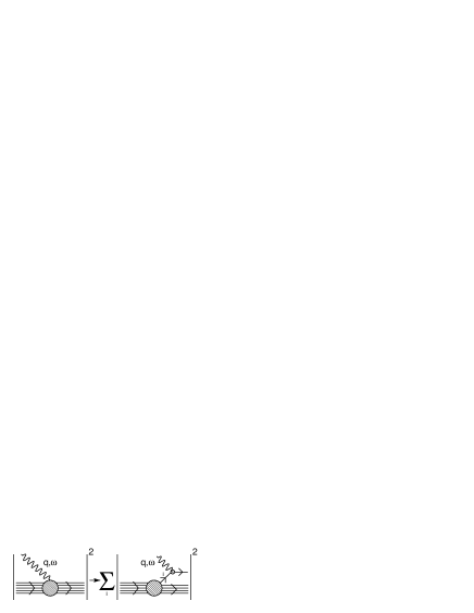
Figure 5: Schematic representation of the IA regime, in which the nuclear cross section is replaced by the incoherent sum of cross sections describing scattering off individual nucleons, the recoiling $({\rm A}-1)$-nucleon system acting as a spectator.

Using Eq. (46) we can replace

$$\sum_{X}|X\rangle\langle X|\rightarrow\sum_{x}\int d^{3}p_{x}|x,{\bf p}_{x}\rangle\langle{\bf p}_{x},x|\sum_{{\cal R}}d^{3}p_{{\cal R}}|{\cal R},{\bf p}_{{\cal R}}\rangle\langle{\bf p}_{{\cal R}},{\cal R}|\ .$$ (47)

Substitution of Eqs. (45)-(47) into Eq. (40) and insertion of a complete set of free nucleon states leads to the factorization of the nuclear current matrix element. As a result, the incoherent contribution to Eq. (40) can be rewritten in the form

$$W^{\mu\nu}({\bf q},\omega)=\int d^{3}k\ dE\ \left(\frac{m}{E_{{\bf k}}}\right)\left[ZP_{p}({\bf k},E)w_{p}^{\mu\nu}({\widetilde{q}})+NP_{n}({\bf k},E)w_{n}^{\mu\nu}({\widetilde{q}})\right]\ ,$$ (48)

where $Z$ and $N=A-Z$ are the number of target protons and neutrons, while $P_{p}$ and $P_{n}$ denote the proton and neutron hole spectral functions, respectively. In Eq. (48), $E_{{\bf k}}=\sqrt{|{\bf k}^{2}|+m^{2}}$ and

$$w_{N}^{\mu\nu}=\sum_{x}\langle{\bf k},{\rm N}|j^{\mu}_{N}|x,{\bf k}+{\bf q}\rangle\langle{\bf k}+{\bf q},x|j^{\nu}_{N}|{\rm N},{\bf k}\rangle\delta({\widetilde{\omega}}+E_{{\bf k}}-E_{x})\ ,$$ (49)

with[1]

$${\widetilde{\omega}}=E_{x}-E_{{\bf k}}=E_{0}+\omega-E_{{\cal R}}-E_{{\bf k}}=\omega-E+m-E_{{\bf k}}\ .$$ (50)

The above equations show that within the IA scheme, the definition of the electron-nucleus cross section involves two elements: i) the tensor $w_{N}^{\mu\nu}$, defined by Eq. (49), describing the electromagnetic interactions of a bound nucleon carrying momentum ${\bf k}$ and ii) the spectral function, discussed in the previous Sections.

4.2 Electron scattering off a bound nucleon

While in electron-nucleon scattering in free space the struck particle is given the entire four momentum transfer $q\equiv(\omega,{\bf q})$, in a scattering process involving a bound nucleon a fraction $\delta\omega$ of the energy loss goes into the spectator system. This mechanism emerges in a most natural fashion from the IA formalism.

Assuming that the current operators are not modified by the nuclear environment, the quantity defined by Eq. (49) can be identified with the tensor describing electron scattering off a free nucleon at four momentum transfer $q\equiv({\bf q},{\widetilde{\omega}})$. Hence, Eq. (49) shows that within IA binding is taken into account through the replacement

$$q\equiv(\omega,{\bf q})\rightarrow{\widetilde{q}}\equiv({\widetilde{\omega}},{\bf q})\ .$$ (51)

The interpretation of $\delta\omega=\omega-{\widetilde{\omega}}$ as the amount of energy going into the recoiling spectator system becomes particularly transparent in the limit $|{\bf k}|/m\ll 1$, in which Eq. (50) yields $\delta\omega=E$.

The tensor $w_{N}^{\mu\nu}$ of Eq. (49) can be obtained from the general expression (compare to Eq. (43))

$$w_{N}^{\mu\nu}=w^{N}_{1}\left(-g^{\mu\nu}+\frac{{\widetilde{q}}^{\mu}{\widetilde{q}}^{\nu}}{{\widetilde{q}}^{2}}\right)+\frac{w^{N}_{2}}{m^{2}}\left(k^{\mu}-\frac{(k{\widetilde{q}})}{{\widetilde{q}}^{2}}{\widetilde{q}}^{\mu}\right)\left(k^{\nu}-\frac{(k{\widetilde{q}})}{{\widetilde{q}}^{2}}{\widetilde{q}}^{\nu}\right)\ ,$$ (52)

where $k\equiv(E_{\bf k},{\bf k})$ and the two structure functions $w_{1}$ and $w_{2}$ can be extracted from the measured electron-proton and electron-deuteron scattering cross sections[27, 28].

For example, in the case of quasielastic scattering $w_{1}$ and $w_{2}$ are simply related to the electric and magnetic nucleon form factors, $G_{E_{N}}$ and $G_{M_{N}}$, through

$$w^{N}_{1}=-\frac{{\widetilde{q}}^{2}}{4m^{2}}\ \delta\left({\widetilde{\omega}}+\frac{{\widetilde{q}}^{2}}{2m}\right)\ G_{M_{N}}^{2}\ ,$$ (53)

$$w^{N}_{2}=\frac{1}{1-{\widetilde{q}}^{2}/4m^{2}}\ \delta\left({\widetilde{\omega}}+\frac{{\widetilde{q}}^{2}}{2m}\right)\left(G_{E_{N}}^{2}-\frac{{\widetilde{q}}^{2}}{4m^{2}}G_{M_{N}}^{2}\right)\ .$$ (54)

A similar expression can be used to describe resonance production. The explicit formula differ in the analytical form of the relevant form factors and for the replacement of the energy conserving $\delta$-function with a Breit-Wigner factor, accounting for the finite width of the resonance.[29] Finally, Eq.(52) can be applied in the region of deep inelastic scattering, where the structure functions $F^{N}_{1}=mw^{N}_{1}$ and $F^{N}_{2}=\omega w^{N}_{2}$ depend on $Q^{2}=|{\bf q}^{2}|-\omega^{2}$ and the bjorken scaling variable $x=Q^{2}/2m\omega$.

As a final remark, it has to be pointed out that the replacement of $\omega$ with $\tilde{\omega}$, while being reasonable on physics grounds, and in fact quite natural in the context of the IA analysis, poses a considerable conceptual problem, in that it leads to a violation of current conservation, that requires

$$q_{\mu}w_{N}^{\mu\nu}=0\ .$$ (55)

However, violation of gauge invariance in the IA scheme turns out to be only marginally relevant to inclusive electron scattering at large momentum transfer. The results of numerical studies suggest that the main effect of nuclear binding can indeed be accounted for with the replacement $\omega\rightarrow{\widetilde{\omega}}$.[1]

4.3 Comparison to electron scattering data

The formalism outlined above, supplemented by the treatment of FSI effects proposed in Refs.[16, 17], has been widely and successfully applied to the analysis of electron-nucleus scattering data.[1]

In Ref. [31], it has been employed to calculate the inclusive electron scattering cross sections off oxygen at beam energies ranging between 700 and 1200 MeV and electron scattering angle 32^∘. In this kinematical region, relevant to many neutrino experiments, single nucleon knock out is the dominant reaction mechanism and both quasi-elastic and inelastic processes, leading to the appearance of nucleon resonaces, must be taken into account.

Comparison between theoretical results and the experimental data of Ref. [30] shows that, while the data in the region of the quasi-elastic peak are accounted for with an accuracy better than $\sim$ 10 %, theory fails to explain the measured cross sections at larger electron energy loss, where $\Delta$ production dominates.

As an example, Fig. 6 shows the results of Ref.[31] at beam energy 700 and 1200 MeV. For reference, the results of the Fermi gas (FG) model corresponding to Fermi momentum $p_{F}=225$ MeV and average removal energy $\epsilon=25$ MeV are also shown. Theoretical calculations have been carried out using the spectral function of Ref.[32], the Höhler-Brash parameterization of the nucleon form factors [33, 34] in the quasi-elastic channel and the Bodek and Ritchie parametrization of the proton and neutron structure functions in the inelastic channels [27].

Figure 6: Cross section of the process ${}^{16}O(e,e^{\prime})$ at scattering angle 32^∘ and beam energy 700 MeV (left panel) and 1200 MeV (right panel), as a function of the electron energy loss $\omega$. Solid lines: full calculation, including FSI. Dot-dash lines: IA calculation. Dashed lines: FG model with $p_{F}=225$ MeV and $\epsilon=25$ MeV. The data are taken from Ref.[30]

The authors of Ref. [31] argued that the disagreement between theory and data in the $\Delta$ production region is likely to be imputable to deficiencies in the description of the neutron structure functions at low $Q^{2}$. This conclusion is supported by the analysis carried out in.[28, 35]

The left panel of Fig. 7 shows that the neutron structure function extracted from Jefferson Lab data at $Q^{2}\sim 0.5$ GeV²[36], following the procedure of Bodek and Ritchie, is significatly larger than the one resulting from the analysis of Ref.[27], based on SLAC data spanning the kinematical domain $1~{}<~{}Q^{2}~{}<~{}20$ GeV². The theoretical cross section obtained using the neutron structure function of Ref.[28], displayed in the right panel, turns out to be in close agreement with the SLAC data of Ref.[37], corresponding to $Q^{2}\sim 0.4$, in the $\Delta$ region.

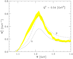
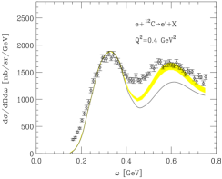
Figure 7: Left panel: nucleon structure functions $w^{N}_{2}$ ($N=n,p$) at $E_{e}=2.445$ GeV and $\theta_{e}=20^{\circ}$, corresponding to $Q^{2}=0.54$ GeV² at the $\Delta$ production peak, plotted as a function of the invariant mass of the hadronic final state. The shaded area represents the $w^{N}_{2}$ resulting from the analysis of Ref.[28], while the dashed and dot-dash lines correspond to $w^{n}_{2}$ and $w^{p}_{2}$ of Ref.[27], respectively. Right panel: electron scattering cross section off carbon at $E_{e}=1.3$ GeV and $\theta_{e}=37.5^{\circ}$, as a function of the electron energy loss $\omega$. The solid line corresponds to theoretical calculations carried out using the proton and neutron structure functions of Ref. [27], while the shaded region has been obtained using $w_{1}^{n}$ and $w_{2}^{n}$ of Ref. [28]. The data are taken from Ref. [37]

5 Charged current neutrino-nucleus interactions

In Born approximation, the cross section of the weak charged current process

$$\nu_{\ell}+A\rightarrow\ell^{-}+X\ ,$$ (56)

can be written in the form (compare to Eq. (38))

$$\frac{d\sigma}{d\Omega_{\ell}dE_{\ell}}=\frac{G^{2}}{32\pi^{2}}\ \frac{|{\bf k}^{\prime}|}{|{\bf k}|}\ L_{\mu\nu}W^{\mu\nu}\ ,$$ (57)

where $G=G_{F}\cos\theta_{C}$, $G_{F}$ and $\theta_{C}$ being Fermi’s coupling constant and Cabibbo’s angle, $E_{\ell}$ is the energy of the final state lepton and ${\bf k}$ and ${\bf k}^{\prime}$ are the neutrino and charged lepton momenta, respectively. Compared to the corresponding quantities appearing in Eq. (38), the tensors $L_{\mu\nu}$ and $W^{\mu\nu}$ include additional terms resulting from the presence of axial-vector components in the leptonic and hadronic currents (see, e.g., Ref. [38]).

Within the IA scheme, the cross section of Eq. (57) can be cast in a form similar to that obtained for the case of electron-nucleus scattering. Hence, its calculation requires the nuclear spectral function and the tensor describing the weak charged current interaction of a free nucleon, $w_{N}^{\mu\nu}$. In the case of quasi-elastic scattering, neglecting the contribution associated with the pseudoscalar form factor $F_{P}$, the latter can be written in terms of the nucleon Dirac and Pauli form factors $F_{1}$ and $F_{2}$, related to the measured electric and magnetic form factors $G_{E}$ and $G_{M}$ through

$$F_{1}=\frac{1}{1-q^{2}/4m^{2}}\left(G_{E}-\frac{q^{2}}{4m^{2}}G_{M}\right)\ \ ,\ \ F_{2}=\frac{1}{1-q^{2}/4m^{2}}\left(G_{M}-G_{E}\right)\ ,$$ (58)

and the axial form factor $F_{A}$.

It has to be pointed out that the formalism described in Section 3, while including dynamical correlations in the final state, does not take into account statistical correlations, leading to Pauli blocking of the phase space available to the knocked-out nucleon.

A rather crude prescription to estimate the effect of Pauli blocking amounts to modifying the spectral function through the replacement

$$P({\bf p},E)\rightarrow P({\bf p},E)\theta(|{\bf p}+{\bf q}|-{\overline{p}}_{F})$$ (59)

where ${\overline{p}}_{F}$ is the average nuclear Fermi momentum, defined as

$${\overline{p}}_{F}=\int d^{3}r\ \rho_{A}({\bf r})p_{F}({\bf r}),$$ (60)

with $p_{F}({\bf r})=(3\pi^{2}\rho_{A}({\bf r})/2)^{1/3}$, $\rho_{A}({\bf r})$ being the nuclear density distribution. For oxygen, Eq. (60) yields ${\overline{p}}_{F}=209$ MeV. Note that, unlike the spectral function, the quantity defined in Eq. (59) does not describe intrinsic properties of the target only, as it depends explicitely on momentum transfer.

The effect of Pauli blocking is hardly visible in the energy loss spectra shown in Fig. 6, as the kinematical setup corresponds to $Q^{2}>0.2$ GeV² at the quasi-elastic peak. However, it becomes appreciable at lower $Q^{2}$.

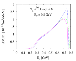
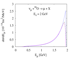
Figure 8: Quasi-elastic differential cross section $d\sigma/dE_{\mu}$, as a function of the charged lepton energy $E_{\mu}$, for neutrino energy $E=$ 0.8 (left panel) and 2.0 GeV (right panel). The solid and dot-dash lines show the results of the IA calculation with and without Pauli blocking (implemented as in Eq. (59)), respsctively. The dashed lines have been obtained using the FG model.

As an example, Fig. 8 shows the $\nu_{\mu}$-nucleus cross sections, as a function of the scattered muon energy, calculated within the FG model (dashed line) and using the the spectral functio of Ref.[32], with and without Pauli blocking (solid and dot-dash lines, respectively). It clearly appears that the FG model yields a larger peak at high-energy. This feature should show up in the cross section at forward angles, and may have a direct effect on neutrino oscillation measurements.

6 Summary

The approach based on NMBT provides a unified parameter-free description of the electroweak nuclear response in a variety of kinematical regions.

Thanks to the availability of reliable spectral functions, accurate calculations of the cross sections in the IA regime can be carried including the effects of short range NN correlations. Correlation effects can also be consistenly included in the treatment of FSI between the struck nucleon and the spectator particles.

Comparison to electron-nucleus scattering data shows that, the region of quasi-elastic scattering and $\Delta$ production can be reproduced with remarkable accuracy. The role of meson exchange currents, which are known to provide a significant amount of strength in the dip region between the quasi-elastic and the $\Delta$ peak, still needs to be carefully investigated. The generalization of the formalism discussed in these lectures to deep inelastic scattering is straightforward.[1]

As a final remark, it has to be pointed out that the possibility of using the approach based on NMBT in the analysis of neutrino experiments largely depends on the ability to implement its elements in Monte Carlo simulations.

Assuming, for the sake of simplicity, that the elementary weak interaction vertex in the nuclear medium be the same as in free space, a realistic simulation of neutrino-nucleus scattering requires the energy and momentum probability distribution of the nucleons, needed to specify the initial state, as well as their distribution in space and the medium modified hadronic cross section, needed for the description of FSI.

Studies based on NMBT and stochastic methods to solve the many-body Schrödinger equation appear to be capable of providing access to all the above quantities for a variety of nuclear targets.

References

- [1] O. Benhar, D. Day and I. Sick, Rev. Mod. Phys., 80 (2008) 189.
- [2] Proceedings of the Fifth International Conference on Perspectives in Hadronic Physics, Edited by C. Ciofi degli Atti and D. Treleani, Nucl. Phys. A 782 (2007).
- [3] Proceedings of The Fifth International Workshop on Neutrino-Nucleus Interactions in the Few-GeV Region (NuInt07), Edited by G.P. Zeller, J.G. Morfin and F. Cavanna (AIP, New York, 2007).
- [4] R.B. Wiringa , V.G.J. Stoks, R. Schiavilla, Phys. Rev. C51 (1995) 38.
- [5] P.S. Pudliner et al, Phys. Rev. C56 (1997) 1720.
- [6] S.C. Pieper and R.B. Wiringa, Ann. Rev. Nucl. Part. Sci. 51 (2001) 53.
- [7] B.D. Day, Rev. Mod. Phys. 39 (1967) 719; ibidem 50 (1978) 495.
- [8] E. Feenberg, Theory of Quantum Fluids, (Academic Press, New York, 1969).
- [9] J.W. Clark, Prog. Part. Nucl. Phys. 2 (1979) 89.
- [10] S. Fantoni and V.R. Pandharipande, Phys. Rev. C 37 (1988) 1697.
- [11] A. Fetter, and J. Walecka, Quantum Theory of Many Particle Systems, (McGraw-Hill, New York, 1971).
- [12] O. Benhar, A. Fabrocini, and S. Fantoni, Nucl. Phys. A 550 (1992) 201.
- [13] O. Benhar, A. Fabrocini, and S. Fantoni, Nucl. Phys. A 505 (1989) 267.
- [14] O. Benhar, A. Fabrocini, and S. Fantoni, Phys. Rev. C 41 (1990) R24.
- [15] W. Dickhoff, and C. Barbieri, Prog. Part. Nucl. Phys. 52 (2004) 377.
- [16] O. Benhar et al, Phys. Rev. C 44 (1991) 2328.
- [17] M. Petraki et al, Phys. Rev. C 67 (2001) 014605.
- [18] V.R. Pandharipande and S.C. Pieper, Phys. Rev. C 45 (1992) 791.
- [19] C. Itzykson and J. Zuber, Quantum Field Theory (McGraw-Hill, New York, 1980).
- [20] J Golak et al., Phys. Rev. C 52 (1995) 1216.
- [21] V.D. Efros, W. Leidemann, and G. Orlandini, Phys. Lett. B338 (1994) 130.
- [22] J. Carlson and R. Schiavilla, Rev. Mod. Phys. 70 (1998 ) 743.
- [23] W. Leidemann, these Proceedings.
- [24] S. Fantoni, and V.R. Pandharipande, Nucl. Phys. A473 (1987) 234.
- [25] A. Fabrocini and S. Fantoni, Nucl. Phys. A503 (1989) 375.
- [26] A. Dellafiore, F. Lenz and F Brieva, Phys. Rev. C 31 (1985) 1088.
- [27] A. Bodek and J. Ritchie, Phys. Rev. D 23 (1981) 1070.
- [28] O. Benhar and D. Meloni, Phys. Rev. Lett. 97 (2006) 192301.
- [29] O. Benhar and D. Meloni, Nucl. Phys. A 789 (2007) 379.
- [30] M. Anghinolfi et al., Nucl. Phys. A 602 (1996) 405.
- [31] O. Benhar et al, Phys. Rev. D 72 (2005) 053005.
- [32] O. Benhar, A. Fabrocini, S. Fantoni and I. Sick, Nucl. Phys. A 579 (1994) 493.
- [33] G. Höhler et al. Nucl. Phys. B 114 (1976) 505.
- [34] E.J. Brash, A. Kozlov, Sh. Li, and G.M. Huber, Phys. Rev. C 65 (2002) 051001(R).
- [35] H. Nakamura, M. Sakuda, T. Nasu and O. Benhar, Phys. Rev. C 76 (2007) 065208.
- [36] I. Niculescu et al, Phys. Rev. Lett. 85 (2000) 1186.
- [37] R.M. Sealock et al, Phys. Rev. Lett. 62 (1989) 1350.
- [38] J.D. Walecka, Theoretical Nuclear and Subnuclear Physics (Oxford University Press, 1995).