Antiproton collisions with molecular hydrogen

Abstract

Theoretical antiproton and proton cross sections for ionization and excitation of hydrogen molecules as well as energy spectra of the ionized electrons were calculated in the impact-energy range from 8 to 4000 keV. The cross sections were computed with the close-coupling formulation of the semi-classical impact-parameter method. The target was described using a one-active electron model centered on the target and assuming a fixed internuclear distance during the collision process. The dependence of the ionization cross sections on the internuclear distance is examined. The present cross sections are compared with experimental and theoretical data from the literature. For impact energies $E\geq 90$ keV the obtained results for ionization by antiproton impact are comparable to the experimental data while they disagree for energies $E<80$ keV.

I Introduction

The ionization of atoms and molecules by antiproton ($\bar{p}$) impacts has become the subject of great theoretical and experimental interest. The motivation for this is twofold. First, there is a fundamental interest in collisions involving exotic particles and second, in comparison to proton ($p$) collisions the sign of the projectile charge is exchanged which opens up the possibility to explore interesting physical effects. Further attention is drawn to this topic due to the upcoming Facility for Antiproton and Ion Research (FAIR) FAIR (2008) (Facility for Antiproton and Ion Research). The international collaborations on atomic and molecular physics FLAIR FLAIR (2008) (Facility for Low-energy Antiproton and Ion Research) and SPARC SPARC (2008) (Stored Particle Atomic Research Collaboration), both being a part of the FAIR project, intend to investigate antiproton driven ionization processes and even kinematically complete antiproton collision experiments Welsch and Ulrich (2007). These experimental efforts complement the recent intense activity in experimental Gabrielse et al. (2002); Amoretti et al. (2002) and theoretical Zygelman et al. (2001); Jonsell et al. (2001, 2004); Armour et al. (2005); Sharipov et al. (2006); Voronin and Froelich (2008) anti-hydrogen studies.

In the last 15 years a large number of elaborate calculations have been carried out for ionization in the simplest one-electron and two-electron systems $\bar{p}$ + H Wells et al. (1996); Schiwietz et al. (1996); Hall et al. (1996); Igarashi et al. (2000); Sakimoto (2000); Pons (2000a, b); Tong et al. (2001); Toshima (2001); Azuma et al. (2001); Sahoo et al. (2004); Sakimoto (2004) and $\bar{p}$ + He Schultz and Krstić (2003); L. A. Wehrman, A. L. Ford and J. F. Reading (1996); Reading et al. (1997); Bent et al. (1998); Lee et al. (2000); Kirchner et al. (2002); Tong et al. (2002); Keim et al. (2003); A. Igarashi, S. Nakazaki and A. Ohsaki (2004); S. Sahoo and Walters (2005); Foster et al. (2008) , respectively, and have offered the single-ionization cross sections in agreement with experimental results Andersen et al. (1986, 1987); Andersen et al. (1990a); Knudsen and Reading (1992); P. Hvelplund and H. Knudsen and U. Mikkelsen and E. Morenzoni and S. P. Møller and E. Uggerhøj and T. Worm (1994); Knudsen et al. (1995) for incident energies $E\geq 50$ keV. An interesting difference between the proton and antiproton impacts was experimentally recognized for the double-ionization cross sections of the He atom Andersen et al. (1986, 1987); P. Hvelplund and H. Knudsen and U. Mikkelsen and E. Morenzoni and S. P. Møller and E. Uggerhøj and T. Worm (1994), and its origin could be explained by theoretical studies Ford and Reading (1994); Knudsen and Reading (1992). At low energies ($E<50$ keV), however, large discrepancies still remained between the experiment and theoretical results both for the single- and double-ionization processes. Very recent experimental results for $\bar{p}$ + He collisions at energies below 30 keV could partly resolve this discrepancies Knudsen et al. (2008). Theoretical work has also been done for other atomic targets, e.g., recently for alkali-metal atoms Lühr and Saenz (2008).

For molecular targets measurements were further made for ionization in $\bar{p}$ + H₂ collisions Andersen et al. (1990b); P. Hvelplund and H. Knudsen and U. Mikkelsen and E. Morenzoni and S. P. Møller and E. Uggerhøj and T. Worm (1994). Again, a notable difference between proton and antiproton impacts could be seen for the ionization cross sections. While detailed work was done for proton impacts Shah and Gilbody (1982); Shah et al. (1989); Rudd et al. (1983, 1985); Elizaga et al. (1999), little is investigated about the ionization of molecules by antiproton impact. In the case of $\bar{p}$ + H₂ collisions a calculation was done by Ermolaev Ermolaev (1993), who used an atomic hydrogen target with a scaled nuclear charge $Z_{\rm n}=1.09\,Z_{\rm proton}$ in order to mimic the H₂ ionization potential. A molecular approach was used by Sakimoto for calculations of the one-electron system $\bar{p}$ + H${}_{2}^{+}$ Sakimoto (2005).

The aim of the present work is to examine the $\bar{p}$ + H₂ collision process in some detail and to improve the existing theoretical cross sections. Therefore, the target molecule is described with an improved model potential in comparison to the simple model used by Ermolaev in Ermolaev (1993). The present model provides cross sections for different internuclear distances of the H₂ molecule. Furthermore, the description of the continuum is improved by expanding the wave functions in B-spline functions as well as by increasing the number of basis states. The paper is organized as follows: Sec. II considers the description of the hydrogen molecule as well as the computational approach. Sec. III reports on the dependence of the ionization cross sections on the molecular internuclear distance. Subsequently, the calculated cross sections for proton and antiproton impact are presented and compared to literature data. Finally, the energy spectra of the ejected electrons are taken into account. Sec. IV concludes on the present findings and discusses the applicability of the used model. Atomic units are used unless it is otherwise stated.

II Method

II.1 Model potential

$R_{n}$	$\alpha$	$I_{p}$[H2]
1.0	0.26255	0.672753
1.2	0.1960	0.635961
1.3	0.1685	0.619606
1.4	0.1440	0.604492
1.4487	0.13308	0.597555
1.5	0.1219	0.590531
1.55	0.1127	0.583959
1.68	0.0881	0.568062
1.8	0.0690	0.554815
2.0	0.0434	0.535499
2.11	0.0313	0.526223

Table 1: Values of the model potential parameter $\alpha$ used in this work for different internuclear distances $R_{n}$ given in  a. u.  For these internuclear distances also the ionization potential $I_{p}$[H₂] for H₂ is given in Hartree which is obtained using the H₂ ground-state potential-energy curve calculated by Wolniewicz Wolniewicz (1993).

The target molecule is treated as an effective one-electron system. The effective electron is exposed to a model potential

$$V_{\rm mod}(r)=-\frac{Z_{n}}{r}\,\left(1+\frac{\alpha}{|\alpha|}\,\exp\,\left[-\frac{2\,r}{|\alpha|^{1/2}}\right]\right)\,,$$ (1)

which contains one dimensionless parameter $\alpha$ and the nuclear charge is $Z_{n}=+1$. It was proposed by Vanne and Saenz in Vanne and Saenz (2008) and further discussed in Lühr et al. (2008). They successfully used $V_{\rm mod}(r)$ for calculating the ionization and excitation of H₂ molecules in intense ultrashort laser pulses. A comparison with their results from a full molecular treatment of H₂ confirmed the applicability of the model for ionization as well as for excitation. The model potential reduces to the ionization potential of atomic hydrogen, $I_{p}[{\rm H}]=0.5$ a. u., for $\alpha\rightarrow 0$. Furthermore, it satisfies the conditions $V_{\rm mod}(r)\rightarrow-1/r$ for $r\rightarrow\infty$ and therefore describes, in contrast to the model used by Ermolaev in Ermolaev (1993), the long-range behavior of the potential correctly.

The dependence of the ionization potential $I_{\rm mod}(\alpha)$ on the parameter $\alpha$ for a system described by $V_{\rm mod}$ is determined numerically in Vanne and Saenz (2008) but for $0\leq\alpha\leq 0.3$ it can also be approximated well with the analytic expression

$$I_{\rm mod}(\alpha)\approx I_{p}[{\rm H}]+\frac{\alpha}{(1+\sqrt{|\alpha|})}\,.$$ (2)

$\alpha$ is chosen such that $I_{\rm mod}$ corresponds to the ionization potential $I_{p}[{\rm H}_{2}]$ of the H₂ molecule at a given internuclear distance $R_{n}$. $I_{p}[{\rm H}_{2}]$ as a function of $R_{n}$ is obtained by subtracting the ground-state potential-energy curve of H₂ which was very accurately calculated by Wolniewicz Wolniewicz (1993) from the ground-state energies of H${}_{2}^{+}$. The values of $\alpha$ used in this work for the various $R_{n}$ ranging from 1.0 a. u. to 2.11 a. u. are given in Table 1 together with the corresponding ionization potentials. It should be mentioned that within this model the effect of anisotropy due to the two nuclei as well as of the second electron is solely contained as a screening of the Coulomb potential.

A different model potential for the target can be obtained if in Eq. (1) the parameter $\alpha$ is set to $\alpha\rightarrow 0$ and the nuclear charge is scaled to $Z_{n}=Z_{\rm scal}=1.09$ as it was, for example, proposed by Ermolaev in Ermolaev (1993). In what follows, it shall be referred to this special case of $V_{\rm mod}$ as $V_{\rm scal}$ which describes a scaled hydrogen atom H_scal with all energy levels shifted according to

$$\epsilon_{j\,}[{\rm H}_{\rm scal}]=(Z_{\rm scal})^{2}\;\epsilon_{j\,}[{\rm H}]\,.$$ (3)

The ionization potential of H_scal is equal to the absolute value of the ground-state energy $I_{p}[{\rm H}_{\rm scal}]=\left|\,\epsilon_{1\,}[{\rm H}_{\rm scal}]\,\right|=0.59405$ a. u. and corresponds to the ionization potential of a H₂ molecule at an internuclear separation $R_{n}=1.474$ a. u.

II.2 Time propagation

An approach similar to the one used in this work was already applied and described in some detail in a previous work Lühr and Saenz (2008) dealing with slow antiproton and proton collisions with alkali-metal atoms. The relative motion of the heavy projectiles is approximated by classical trajectories with constant velocities ${\bf v}_{p}$ parallel to the $z$ axis also known as the impact-parameter method. The distance vector $\mathbf{R}$ between the projectile and the target is given by

$${\mathbf{R}(t)=\mathbf{b+v}_{p}}\,t\,,$$ (4)

where $\mathbf{b}$ is the impact-parameter vector along the $x$ axis and $t$ the time. The internuclear distance $R_{n}$ of the two molecular target nuclei is held fixed during the collision process. The time-dependent Schrödinger equation

$$i\,\frac{\partial}{\partial t}\,\Psi({\bf r},t)=\left(\,\hat{H}_{0}+\hat{V}_{\rm int}({\mathbf{r,R}}(t))\,\right)\,\Psi({\bf r},t)\,$$ (5)

of the target interacting with the projectile is solved. $\hat{H}_{0}$ is the Hamiltonian of the effective target electron including the model potential (1)

$$\hat{H}_{0}=-\frac{1}{2}\nabla^{2}+\hat{V}_{\rm mod}\,.$$ (6)

The time-dependent interaction between the projectile with the charge $Z_{p}$ and the target is given by the time-dependent interaction potential

$$V_{\rm int}({\mathbf{r,R}}(t))=\frac{-Z_{p}}{\left|\mathbf{r-R}(t)\right|}+\frac{Z_{p}}{|\mathbf{R}(t)|}\,,$$ (7)

where ${\bf r}$ is the spatial coordinate of the effective electron. The time-dependent wavefunction

$$\Psi({\bf r},t)=\sum_{j}\,c_{j}(t)\,\phi_{j}(\mathbf{r})\,\exp[-i\,\epsilon_{j}\,t]$$ (8)

is expanded in eigenstates $\phi_{j}$ of the target Hamiltonian $\hat{H}_{0}$ with the energies $\epsilon_{j}$. The radial part of $\phi_{j}$ is furthermore expanded in $B$-spline functions whereas its angular part is expanded in spherical harmonics. Substitution of the wavefunction $\Psi$ in Eq. (5) by its expansion given in Eq. (8) results for a trajectory with fixed $b$ (cf. Eq. (4)) in a system of coupled differential equations

$$i\frac{\textrm{d}}{\textrm{d}t}\,c_{j}(t,b)=\sum_{k}c_{k}(t,b)\,\langle\phi_{j}|\hat{V}_{\rm int}|\phi_{k}\rangle\exp[i(\epsilon_{j}-\epsilon_{k})t]\,.$$ (9)

The differential equations (9) are solved with the initial conditions ${c_{j}({t=-\infty};b)}=\delta_{j\,1}$, where $c_{1}$ is the coefficient of the ground state of the target Hamiltonian $\hat{H}_{0}$. The transition probability $P_{j}(b)$ for a transition into the target state $j$ after a collision with the impact parameter $b$ is given by

$$P_{j}(b)=|c_{j}(t=+\infty,b)|^{2}$$ (10)

and accordingly the probabilities for ionization $P_{\rm ion}(b)$ and excitation $P_{\rm ex}(b)$ by

$$P_{\rm ion}(b) = \quad\sum_{\epsilon_{j}>0}|c_{j}(t=+\infty,b)|^{2}\,,$$ (11)

$$P_{\rm ex}(b) = \sum_{\epsilon_{1}<\epsilon_{j}<0}|c_{j}(t=+\infty,b)|^{2}\,.$$ (12)

The cross section for the transition into the target state $j$ can be expressed as

$$\sigma_{j}=2\,\pi\,\int P_{j}(b)\,b\;\textrm{d}b\,.$$ (13)

For an H₂ target the cross section for ionization is defined as

$$\sigma_{\rm ion}=2\,\pi\,\int 2\,P_{\rm ion}(b)\,b\;\textrm{d}b$$ (14)

and for excitation as

$$\sigma_{\rm ex}=2\,\pi\,\int 2\,P_{\rm ex}(b)\,b\;\textrm{d}b\,.$$ (15)

The electron-energy spectrum

$$S(\epsilon)=\frac{\textrm{d}\sigma_{\rm ion}(\epsilon)}{\textrm{d}\epsilon}=2\,\sum_{\epsilon_{j}=\epsilon}\rho\;\!(\epsilon_{j})\;\sigma_{j}\,,$$ (16)

that is the differential cross section for ejecting an electron with an energy $\epsilon$, can be obtained by using the density of the continuum states $\rho$. The factor two in Eqs. (14–16) accounts for the two indistinguishable electrons of the H₂ molecule. The introduction of such a simple factor is believed to work as long as independent interactions of the electrons with the projectile are dominating. This is the case for high projectile velocities. However, it is unclear to what extend phenomena including electron-electron-interaction like double-ionization can be described with an effective one-electron model and furthermore can be extracted from the determined transition probabilities (Eqs. (10) to (11)) and therfore are not considered here.

III Results and discussion

III.1 Dependence of the internuclear distance

Figure 1: Ionization cross section $\sigma_{\rm ion}(R_{n})$ for $\bar{p}$ + H₂ as a function of the internuclear distance $R_{n}$ at $E$ = 16, 64, 125, 250, 1000, and 4000 keV.

The calculated cross sections depend primarily on the ionization potential which in turn depends for the H₂ molecule on the internuclear distance $R_{n}$ (cf. Table 1). A cross section $\sigma(R_{n})$ which depends on $R_{n}$ may therefore be defined as

$$\sigma\>\!(\>\!R_{n}\>\!)\equiv\sigma\>\!\left(\;\!I_{p}[{\rm H}_{2}]\>\!(R_{n})\;\!\right)\,.$$ (17)

As has been shown for $\bar{p}$ + H${}_{2}^{+}$ collisions by Sakimoto Sakimoto (2005) who used a full description of the molecular target ion the dependence of $\sigma_{\rm ion}(R_{n})$ on $R_{n}$ in the range $1.5{\rm{\rm\,a.\,u.}}\leq R_{n}\leq 3.0$ a. u. differs for parallel and perpendicular orientations. For an orientation of the molecular ion perpendicular to the collision plane the dependence on $R_{n}$ is rather weak. Whereas for an orientation parallel to the trajectory of the projectile the ionization cross sections increase approximately linearly for larger $R_{n}$ by more than a factor two in the given $R_{n}$ range. A stronger orientational dependence is expected for H${}_{2}^{+}$ cations compared to a H₂ molecule because of their larger equilibrium internuclear distance. Necessarily, no molecular-orientation dependence is taken into account in the present study. Since the present cross sections depend according to Eq. 17 on the ionization potential which is orientation-independent the present results are interpreted as orientation-averaged.

Fig. 1 shows the present $\bar{p}$ + H₂ ionization cross sections $\sigma_{\rm ion}(R_{n})$ for the impact energies $E$ = 16, 64, 125, 250, 1000, and 4000 keV as a function of $R_{n}$. Ionization cross sections were calculated for eleven different internuclear distances in the range $1.0{\rm\,a.\,u.}\leq R_{n}\leq 2.11$ a. u.  It can be seen that for all impact energies shown here the ionization cross sections increase with larger $R_{n}$. This can be explained with the decrease of the ionization potential for an increasing internuclear distance also shown in Table 1. The dependence of $\sigma_{\rm ion}$ on $R_{n}$, however, diminishes with higher impact energies. For energies $E\geq 1000$ keV $\sigma_{\rm ion}(R_{n})$ depends only weakly on $R_{n}$ and increases by about a factor 1.2 in the whole $R_{n}$ range. For smaller energies $E\leq 125$ keV the dependence on the internuclear distance is much stronger and for $E=16$ keV $\sigma_{\rm ion}(R_{n})$ increases by more than a factor 1.7 in the considered $R_{n}$ range. Furthermore, for all considered impact energies the cross sections show roughly a linear dependence on $R_{n}$. Therefore, one may assume that for all impact energies $E$ considered in the present investigation the simple relation

$$\sigma_{\rm ion}(R_{n})=\sigma_{\rm ion}(\,\overline{R_{n}}\,)+\left(R_{n}-\overline{R_{n}}\,\right)\left.\frac{\textrm{d}\sigma_{\rm ion}(R_{n})}{\textrm{d}R_{n}}\right|_{\,\overline{R_{n}}}$$ (18)

holds approximately in the examined interval where $\overline{R_{n}}$ is a fixed internuclear distance within this interval.

In Fig. 2 ionization probabilities $P_{\rm ion}(b)$ weighted with the impact parameter $b$ as a function of $b$ are compared for four different internuclear distances $R_{n}$ = 1.2, 1.5, 1.8, and 2.11 a. u. at two antiproton impact energies $E$ = 125 keV and 1000 keV. It can be seen that the curves for the higher impact energy $E$ = 1000 keV differ much less than those for $E$ = 125 keV in accordance with Fig. 1. All maxima of the curves for $E$ = 1000 keV lie around $b=1.3$ a. u.  The maxima for $E$ = 125 keV slightly move from $b=1.0$ a. u. for $R_{n}=1.2$ a. u. towards $b=1.3$ a. u. for $R_{n}=2.11$ a. u. and thereby also increase in height. Whereas, the qualitative behavior of the curves for a considered impact energy does not change for varying $R_{n}$.

In order to determine results which include the rovibrational motion of the H₂ molecule one may use the fact that the cross sections to a given electronic state can be correctly given using closure (cf. Saenz and Froelich (1997))

$$\sigma=\int_{0}^{\infty}\sigma(R_{n})\,\left|\,\frac{\xi_{0}(R_{n})}{R_{n}}\,\right|^{\,2}(R_{n})^{\,2}\ \textrm{d}R_{n}\,,$$ (19)

where $\xi_{0}(R_{n})/R_{n}$ is the radial nuclear wave function of an H₂ molecule in its rovibronic ground state. Clearly, the integration in Eq. (19) leads to a loss of the electron-energy resolution. The energy information, however, is not relevant for integrated cross sections $\sigma$ but for differential cross sections like the electron-energy spectrum ${\rm d}{\sigma}\,/\,{\rm d}{\epsilon}$.

It is always possible to express $\sigma(R_{n})$ in terms of an (infinite) polynomial in $R_{n}$ and therefore to reformulate Eq. (19) as

$$\sigma = \int_{0}^{\infty}\left(\sum_{k=0}^{\infty}a_{k}\,(R_{n})^{\,k}\right)\left|\,\xi_{0}(R_{n})\,\right|^{\,2}\ \textrm{d}R_{n}$$ (20)

$$= \sum_{k=0}^{\infty}a_{k}\,\int_{0}^{\infty}(R_{n})^{\,k}\,\left|\,\xi_{0}(R_{n})\,\right|^{\,2}\ \textrm{d}R_{n}$$ (21)

$$= \sum_{k=1}^{\infty}a_{k}\,\left\langle\,(R_{n})^{\,k}\,\right\rangle+a_{0}\,,$$ (22)

where $\left\langle\,(R_{n})^{\,k}\,\right\rangle$ denotes the expectation value of ${(R_{n})^{\,k}}$ for the rovibrational ground state of H₂. If the cross section $\sigma(R_{n})$ depends on $R_{n}$ linearly, which is here at least to a good extend the case, one finds, using Eqs. (18) and (22), the special relation

$$\sigma=a_{1}\,\left\langle\,R_{n}\,\right\rangle+a_{0}=\sigma\left(\left\langle\,R_{n}\,\right\rangle\right)\,,$$ (23)

i.e., it is sufficient to evaluate the cross section at the expectation value of the internuclear distance $\left\langle\,R_{n}\,\right\rangle$ of the H₂ molecule. The value $\left\langle\,R_{n}\,\right\rangle=1.448$ a. u. has been reported by Kolos and Wolniewicz Kolos and Wolniewicz (1964) and it was used in the present calculations to determine the ionization and excitation cross sections.

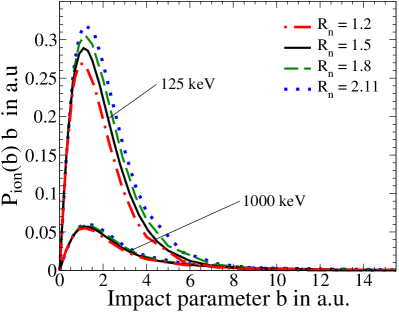
Figure 2: (Color online) Ionization probability $P_{\rm ion}(b)$ weighted with the impact parameter $b$ as a function of $b$ at two different antiproton impact energies $E$ = 125 keV and 1000 keV. Curves for four different internuclear distances $R_{n}$ are compared [in  a. u.]: 1.2 (dot-dashed curve), 1.5 (solid curve), 1.8 (dashed curve), and 2.11 (dotted curve).

It may be mentioned that although the vibration and rotation of the H₂ molecule is taken into account a distortion of the molecular vibration and rotation during the collision with the projectile may possibly lead to a substantial change in magnitude of the cross section. The effect of such a distortion (which is not accounted for in the present work) on $\sigma$ may be largest for small impact energies where the cross section depends considerably on $R_{n}$ as has been shown in Fig. 1. In order to better understand collision processes involving slow antiprotons ($E<100$ keV) it would be desirable to fully include, in an advanced approach, the evolution of the internuclear distance during the collision.

III.2 Ionization of H₂ by $p$ impact

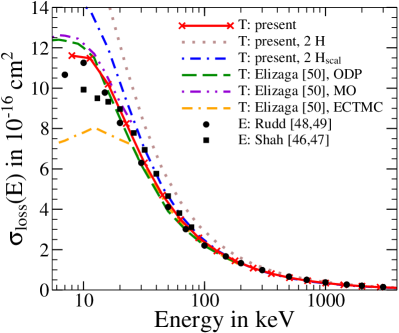
Figure 3: (Color online) Electron-loss cross sections $\sigma_{\rm loss}$ for $p$ + H₂ as a function of the impact energy $E$. Theory. Present results: solid curve, $p$ + H₂; dotted curve, $p$ + H multiplied by two; dash–dotted curve, $p$ + H_scal multiplied by two. Elizaga et al. Elizaga et al. (1999): dashed curve, optimized dynamical pseudostates method; dash–double-dotted curve, molecular orbitals method; double-dash–dotted curve, eikonal classical trajectory Monte Carlo method. Experimental results: filled circles, Rudd et al. Rudd et al. (1983, 1985); filled squares, Shah and Gilbody Shah and Gilbody (1982); Shah et al. (1989).

As has been discussed in a previous work Lühr and Saenz (2008) in some detail much more effort is needed to bring proton compared to antiproton cross sections to convergence using the present method. This is in particular true for low proton impact energies where electron capture becomes the dominant loss channel of the target electrons. The difficulties in the description of the electron capture are mainly due to the use of a one-center expansion of the basis around the target which has to be compensated with an enlarged basis set. The main motivation for the present calculations of proton results is given by the need for a comparison of the employed method with an extended amount of literature since the experimental and theoretical data on antiproton collisions with H₂ molecules are still sparse. A one-center expansion around the target, however, seems to be justified for antiproton collisions in which electron capture is absent and which are in the focus of this investigation.

The present results for the electron loss of molecular hydrogen in collisions with protons are shown in Fig. 3 as a solid curve. Also shown are the electron-loss cross sections for atomic hydrogen in a $p$ + H collision multiplied by two. The present data are compared with experimental results by Rudd et al. Rudd et al. (1983, 1985) and by Shah and Gilbody Shah and Gilbody (1982); Shah et al. (1989).

The present findings for H₂ match the experimental data by Rudd et al. in the whole energy range. The agreement with the measurements of Shah and Gilbody is also good except for $E<20$ keV where their data starts to be smaller than the results of the present work as well as those of Rudd et al. The electron loss cross sections for an atomic hydrogen target in $p$ + H collisions multiplied by two agree well with the experimental and present data for $E>300$ keV. With decreasing impact energies, i.e., with increasing dependence of the cross sections on the internuclear distance, the results for $p$ + H get, however, considerably too large.

In the theoretical work by Elizaga et al. Elizaga et al. (1999) a similar model potential was used which can be obtained by integrating an effective hydrogen atom-like charge distribution with Gauss’s theorem. This model potential was also proposed by Hartree in Hartree (1957) for He atoms ($R_{n}=0$). Cross sections for the electron loss were calculated for $R_{n}=1.4$ a. u.  Thereby, the three methods molecular orbitals (MO), optimized dynamical pseudostates (ODP), and eikonal classical trajectory Monte Carlo (ECTMC) were used in the calculations and the results are also shown in Fig. 3. The cross sections obtained with ODP are very similar to the present ones. Only for $E<10$ keV they are larger than the present data and those by Rudd et al. The MO approach was applied only at low energies $E<25$ keV and leads throughout to similar, though, slightly larger results than those obtained with ODP. Exactly in the latter energy range the outcome obtained with ECTMC differs considerably from all other curves whereas for $E>25$ keV it matches the experimental and the present results very well. It can be concluded that the present approach is capable of describing collisions with H₂ targets quite accurately in the considered energy range.

III.3 Ionization of H₂ by $\bar{p}$ impact

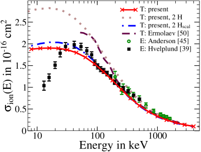
Figure 4: (Color online) Ionization cross section $\sigma_{\rm ion}$ for $\bar{p}$ + H₂ as a function of the impact energy $E$. Theory: solid curve, present results; dotted curve, present results for $\bar{p}$ + H multiplied by two; dash-dotted curve, present results for $\bar{p}$ + H_scal multiplied by two; dashed curve, results for $\bar{p}$ + H_scal multiplied by two by Ermolaev Ermolaev (1993). Experiment: circles, Anderson et al. Andersen et al. (1990b); squares, Hvelplund et al. P. Hvelplund and H. Knudsen and U. Mikkelsen and E. Morenzoni and S. P. Møller and E. Uggerhøj and T. Worm (1994).

The present results for the ionization of molecular hydrogen by antiproton impact are shown in Fig. 4 as solid curve. Also shown are the ionization cross sections for antiproton collisions with atomic hydrogen multiplied by two. The results are compared with calculations by Ermolaev Ermolaev (1993) and experimental data for non-dissociative ionization by Anderson et al. Andersen et al. (1990a) as well as data of a subsequent measurement by Hvelplund et al. P. Hvelplund and H. Knudsen and U. Mikkelsen and E. Morenzoni and S. P. Møller and E. Uggerhøj and T. Worm (1994). As has been suggested by Hvelplund et al. in P. Hvelplund and H. Knudsen and U. Mikkelsen and E. Morenzoni and S. P. Møller and E. Uggerhøj and T. Worm (1994) the data for impact energies below 200 keV of their earlier measurement Andersen et al. (1990a) are omitted in Fig. 4. The data for $E<200$ keV of their first experiment are generally some $10\%$ larger than those in P. Hvelplund and H. Knudsen and U. Mikkelsen and E. Morenzoni and S. P. Møller and E. Uggerhøj and T. Worm (1994) but have a considerably lower accuracy.

For high impact energies $E\geq 1000$ keV all theoretical curves coincide and also agree with the experimental data. For lower energies ($400\,{\rm keV}<E<1000$ keV) the ionization cross sections for atomic hydrogen start to differ from both theoretical results for a hydrogen molecule. However, at these energies the atomic results seem to describe better the experimental data. In the energy regime from 250 keV down to 90 keV the theoretical cross sections by Ermolaev approach those of the $\bar{p}$ + H calculation which differ significantly from the measured cross sections. The experimental data are, however, well described by the present $\bar{p}$ + H₂ cross section in this energy regime. Though, the strong variation of the experimental data around 85 keV is not followed by the smooth curve of the present results. While the magnitude of the present cross sections is comparable to the experimental data down to 20 keV the functional behavior of both, experimental and present curve, starts to differ for $E<50$ keV. Here, the present $\bar{p}$ + H₂ curve possesses a similar characteristic as two times the cross sections of the hydrogen atom but with smaller magnitude because of the larger ionization potential of the molecule. The slope of the present cross sections at these low energies may indicate the lack of two-electron effects in the target description. The experimental data, on the other hand, show a behavior very similar to that of the single ionization of helium also measured with the same experimental set-up by Hvelplund et al. P. Hvelplund and H. Knudsen and U. Mikkelsen and E. Morenzoni and S. P. Møller and E. Uggerhøj and T. Worm (1994). Very recently the same authors published another measurement of the single ionization cross section for $\bar{p}$ + H₂ in the energy range $3\,{\rm keV}<E<25$ keV Knudsen et al. (2008) which revealed that their helium single ionization cross sections in P. Hvelplund and H. Knudsen and U. Mikkelsen and E. Morenzoni and S. P. Møller and E. Uggerhøj and T. Worm (1994) are too small for the lowest measured energies. It may be an interesting question whether the same is true in the case of the $\bar{p}$ + H₂ ionization cross sections as suggested by the present results. Therefore, it would be worthwhile to initiate a further attempt to measure $\bar{p}$ + H₂ cross sections at low antiproton energies.

An effective one-electron description with a fixed internuclear distance seem to be sufficient to describe non-dissociative ionization cross sections for $\bar{p}$ + H₂ at high energies. But it is unclear how strong the influence of two-electron effects and the variation of the internuclear distance is at intermediate and low energies. Since the energy regime around and below the maximum of the ionization cross section is considered to contain interesting physical effects a full quantum mechanical treatment of the target molecule would be desirable. It should be mentioned, however, that such an approach is very demanding.

III.4 Excitation of H₂ by $\bar{p}$ impact

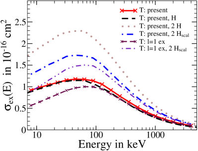
Figure 5: (Color online) Excitation cross section $\sigma_{\rm ex}$ for $\bar{p}$ + H₂ as a function of the impact energy $E$. Theory: solid curve, present results; long-dashed curve, results for $\bar{p}$ + H; dotted curve, same results for $\bar{p}$ + H multiplied by two; dash-dotted curve, results for $\bar{p}$ + H_scal multiplied by two. Cross sections for excitation into $l=1$ states. Theory: thin short-dashed curve, present results; thin dash-double-dotted curve, results for $\bar{p}$ + H_scal multiplied by two.

The present excitation cross sections for $\bar{p}$ + H₂ are shown in Fig. 5 as solid curve. Also shown are results for antiproton collisions with atomic hydrogen and the same atomic cross sections multiplied by two. To the best of the authors’ knowledge there are no data in literature to compare these results with.

Due to the experiences with the ionization cross sections one may estimate the range of validity of the excitation cross sections presented here to be about $100\,{\rm keV}\leq E\leq 4000$ keV. Comparing the results for ionization and excitation in $\bar{p}$ + H₂ collisions one can say that $\sigma_{\rm ex}$ is smaller than $\sigma_{\rm ion}$ for impact energies $E<1000$ keV and that both are practically the same for larger energies. The maximum of $\sigma_{\rm ex}(E)$ lies around $E=58$ keV and therefore at a higher energy than the maximum for ionization.

The excitation cross sections for molecular hydrogen can also be compared with the results for atomic hydrogen. Fig. 5 clearly shows that the naive assumption an H₂ molecule is essentially composed of two independent hydrogen atoms yields excitation cross sections which are obviously different from those which were obtained with the model potential $V_{\rm mod}$ given in Eq. (1). Only for high impact energies both curves get close to each other. On the other hand, it is interesting to observe that the excitation cross sections for a single hydrogen atom seem to be much more in accordance with the present molecular $\sigma_{\rm ex}$. Both cross sections show the same behavior and have practically the same values in the considered energy range. This similarity for atomic and molecular hydrogen targets was evidently not found in the case of ionization in Sec. III.3.

III.5 Electron spectra

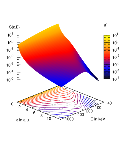
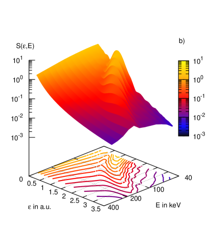
Figure 6: (Color online) Electron-energy spectra surface $S(\epsilon,E)=\textrm{d}\sigma(\epsilon,E)\,/\,\textrm{d}\epsilon$ given in 10^-16 cm² /  a. u. as a function of the electron energy $\epsilon$ in hartree and the impact energy of the antiproton $E$ in keV.  a) $\bar{p}$ + H₂;  b) $p$ + H₂.

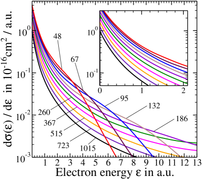
Figure 7: (Color online) Electron-energy spectra curves $S(\epsilon)=\textrm{d}\sigma(\epsilon)\,/\,\textrm{d}\epsilon$ for $\bar{p}$ + H₂ as a function of the electron energy $\epsilon$ at $E$ = 48, 67, 95, 132, 186, 260, 367, 515, 723, and 1015 keV. The inset shows the spectra for the range 0 $\leq$ $\epsilon$ $\leq$ 2 a. u. without scaling the $y$ axis. The curves in the inset are order accordingly to the impact energy $E$. The uppermost curve belongs to the smallest (48 keV) and the lowest curve to the highest (1015 keV) impact energy $E$.

The electron-energy spectra $S(\epsilon,E)=\textrm{d}\sigma(\epsilon,E)\,/\,\textrm{d}\epsilon$ of ionized electrons in a $\bar{p}$ + H₂ collision are presented in Fig. 6a as a function of the electron energy $\epsilon$ and the impact energy of the antiprotons $E$. As has been mentioned before, the disadvantage of the closure approach in Eq. (19) lies in the loss of the detailed electron-energy information of the transitions probabilities which is of relevance to the electron-energy spectra (cf. Saenz and Froelich (1997)). Therefore, the presented results may be interpreted as electron spectra for a fixed internuclear distance rather than including the full rovibrational motion of the nuclei as it is the case for the integrated cross sections which have been discussed before. The electron spectra are calculated for a wide electron-energy range $0<\epsilon<12{\rm\,a.\,u.}$ and for different impact energies of the antiproton ranging from 48 keV to 1015 keV. The contour plot on the bottom of Fig. 6a shows the corresponding level curves and gives therefore information on the gradient of the spectra surface. It can be seen that within the whole impact-energy range the electron spectra decrease smoothly and monotonically for increasing $\epsilon$. Considering small electron energies $\epsilon<2$ a. u., the spectra fall off strongly in view of the logarithmic scale for all impact energies. Within this $\epsilon$ interval, Fig. 6a shows that the smaller the impact energies $E$ the larger the values of $S(\epsilon,E)$. However, for larger $\epsilon$ this uniform trend starts to cease. For $\epsilon>4$ a. u. the overall decrease becomes weaker. Though, the electron spectra for small $E$ start to decrease again very strongly where the fall-off of the spectra is the steepest for the smallest $E$. Consequently, in the intervals of $\epsilon$ and $E$ considered here, the largest value of $S(\epsilon,E)$ for a given $\epsilon$ moves from $E=48$ keV at $\epsilon=0$ to $E\approx 200$ keV at $\epsilon=12$ a. u.

Cuts $S(\epsilon)$ of the same electron-spectra surface for ten different antiproton impact energies $E$ = 48, 67, 95, 132, 186, 260, 367, 515, 723, and 1015 keV are presented in Fig. 7. The inset shows the same $S(\epsilon)$ curves in an interval of small electron energies 0 $\leq$ $\epsilon$ $\leq$ 2 a. u. Thereby, the scaling of the $y$ axis of the inset is kept as it is the main graph. The ordering of the $S(\epsilon)$ curves in the inset is according to their impact energy $E$, i.e., the uppermost curve is the one for the smallest (48 keV) and the lowest curve the one for the largest (1015 keV) impact energy $E$. It can be seen that no crossings of the electron-spectra curves $S(\epsilon)$ occur in this low electron-energy regime.

In contrast to the behavior for small $\epsilon$ shown in the inset the $S(\epsilon)$ curves start to cross each other at higher electron energies. The curve for $E=48$ keV starts to fall off much steeper than the other $S(\epsilon)$ curves for $\epsilon>3$ a. u. and therefore crosses all lower lying curves. Its first crossing takes place at $\epsilon\approx 3.19$ a. u. while its last crossing occurs at $\epsilon\approx 6.13$ a. u.  with the curve for $E=1015$ keV. The other electron-energy curves for higher antiproton impact energies share the same characteristics, namely, that the curve with the largest values of $S(\epsilon)$ in a certain $\epsilon$ range starts to fall off steeper than all other lower lying spectra curves for higher impact energies. Though, with increasing impact energies $E$ the decline of the $S(\epsilon)$ curves starts at larger $\epsilon$ and gets less steep.

For comparison to the antiproton results in Fig. 6a an electron-energy spectra surface $S(\epsilon,E)$ is also presented for $p$ + H₂, i.e., for proton impact, in Fig. 6b. The electron spectra are given for the electron-energy range $0<\epsilon<3.5{\rm\,a.\,u.}$ and for proton impact energies from 48 keV to 310 keV. In general the values of $S(\epsilon,E)$ decrease for larger $\epsilon$. However, the most striking feature of Fig. 6b, in contrast to the case of antiproton impact, is the existence of local maxima of the spectrum curves $S(\epsilon)$ for a given impact energy $E$ which are also visible in the contour plot on the bottom of the figure. The position of the peaks of $S(\epsilon,E)$ varies with the impact energy $E$. At the center of the maxima the ratios of the two energies $E$ and $\epsilon$ are such that the classical velocities of the proton $v_{p}$ and of the electron $v_{e}$ are equal, i.e.,

$$\sqrt{\frac{2\,E}{M_{p}}}=v_{p}=v_{e}=\sqrt{{2\,\epsilon}}\,,$$ (24)

which can be reformulated as

$$\epsilon=\frac{E}{M_{p}}=\frac{1}{2}\,(v_{p})^{2}\,,$$ (25)

where $M_{p}$ is the proton mass. The accuracy of this statement is demonstrated in Fig. 8 where the present $S(\epsilon)$ spectrum curve for protons with an impact energy $E=48$ keV, i.e. $v_{p}=1.3856$ a. u., is shown as solid curve. The maximum of $S(\epsilon)$ is located at $\epsilon=\frac{1}{2}\,(v_{p})^{2}=0.96$ a. u., also indicated by the vertical line.

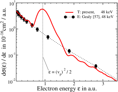
Figure 8: (Color online) Electron-energy spectra curve $S(\epsilon)=\textrm{d}\sigma(\epsilon)\,/\,\textrm{d}\epsilon$ for $p$ + H₂ as a function of the electron energy $\epsilon$ at $E$ = 48 keV. Theory: solid curve, present results for electron loss. Experiment: filled circles, results for ionization, Gealy et al. Gealy et al. (1995). The energy $\epsilon$ of an electron with the velocity of the proton $v_{p}$ is indicated by the vertical line.

The occurring maxima can be explained with the simple picture of the electron-capture process where the electron is captured by the proton and moves basically with the momentum of the projectile. Therefore, the velocity of the captured electron relative to the H₂ molecule is given by the velocity of the projectile, namely the proton, as well as the electron velocity relative to the moving rest frame of the projectile. Since both contributions to the electron momentum can be oriented in different directions the peaks of the electron spectra $S(\epsilon)$ are centered around the energy $\epsilon$ which corresponds to a free electron with the velocity of the projectile, cf. Eq. (25). It may be mentioned that the capture peaks get much less pronounced for higher impact energies. This is, first, due to the diminishing probability of capture for larger $E$ and, second, due to a broader $\epsilon$ distribution of the captured electrons.

If the discussed maxima of $S(\epsilon,E)$ in Fig. 6b are removed one is left with a smoothly decreasing electron-spectra surface $S_{\rm nc}(\epsilon,E)$ for increasing $\epsilon$ which is similar to the one for antiproton impact in Fig. 6a. This modified $S_{\rm nc}(\epsilon,E)$ for proton impact may be interpreted as the electron-energy spectrum surface where the electron capture by the projectile is excluded. In Fig. 8 the present $S(\epsilon)$ curve for a proton impact energy $E=48$ keV is compared with experimental data by Gealy et al. Gealy et al. (1995) for which capture is excluded. The comparison shows that except for the $\epsilon$ regime where capture is the dominant process, i.e. $0.6>\epsilon>1.6$, the present results agree with the experimental data though they underestimate the experimental findings for high electron energies. The integral of the difference between the present and the experimental curve over $\epsilon$ ( $\approx 2.2\times 10^{-16}$ cm²) yields the capture probability for $E=48$ keV calculated by Shingal and Lin Shingal and Lin (1989) ($\approx 2\times 10^{-16}$ cm²) to a good extend. The reason for the structures of the theoretical curve for energies close to the capture peak is not exactly known. It is likely that they originate from the finiteness of the numerical description.

III.6 Comparison of the models $V_{\rm mod}$ and $V_{\rm scal}$

To the best of the authors’ knowledge the only existing calculation for $\bar{p}$ + H₂ collisions was performed by Ermolaev who used the potential $V_{\rm scal}$ to describe the target which is basically an atomic hydrogen target H_scal with a scaled nuclear charge $Z_{n}=1.09$. His results, shown in Fig. 4, are not conform with the experimental data and the present findings. In order to find out why the one model $V_{\rm mod}$ yields much better results than the other and whether the same disagreement occurs also for $p$ impact the same cross sections were calculated again for $p$ and $\bar{p}$ collisions but using $V_{\rm scal}$ in order to describe the target. The resulting cross sections for $\bar{p}$ and $p$ impact multiplied by the factor two are also shown in Figs. 3 to 5 as dash-dotted curves. In what follows three remarks shall be made concerning the results of the calculations using the scaled hydrogen potential $V_{\rm scal}$.

First, it is obvious that the present results for ionization in $\bar{p}$ + H_scal collisions shown in Fig. 4 clearly deviate from those of Ermolaev Ermolaev (1993). It is astonishing that the latter results by Ermolaev better match the present data for unscaled atomic hydrogen than the present and experimental data for molecular hydrogen. No detailed information is given in Ermolaev (1993) concerning the employed basis set and the convergence of the calculations. In very similar studies by Ermolaev Ermolaev (1990a, b), however, a two-center Slater-type orbital expansion with 51 basis functions were applied to describe the collision process between $p$ and $\bar{p}$ projectiles and (unscaled) hydrogen atom targets. It may be mentioned that the quality of the continuum description in the calculations by Ermolaev has been put into question by other authors P. Hvelplund and H. Knudsen and U. Mikkelsen and E. Morenzoni and S. P. Møller and E. Uggerhøj and T. Worm (1994); Toshima (1993), especially in the so-called ’polarization region’, i.e. between $\sim\!70$ and 500 keV.

Second, the present ionization cross sections using $V_{\rm mod}$ and $V_{\rm scal}$ as target potentials both yield, especially for $E>100$ keV, comparable results which can be seen in Figs. 3 and 4 for $p$ and $\bar{p}$ impact, respectively. Deviations become visible for $E<100$ keV. The similar behavior may be explained with their comparable ionization potentials $I_{\rm mod}=0.5976$ a. u. at $R_{n}=\left\langle\,R_{n}\,\right\rangle$ and $I_{p}[{\rm H_{scal}}]=0.5945$ a. u.

Third, the present cross sections for excitation in Fig. 5 differ, however, considerably for $V_{\rm mod}$ and $V_{\rm scal}$. To the best of the authors knowledge no literature data exists to compare the present results with and therefore to judge which of both models is superior in describing excitation of H₂ molecules. On the other hand it has been observed that the excitation cross sections of alkali-metal atoms depend considerably on the energy difference $\Delta\epsilon$ between the energetically lowest dipole-allowed $p$ states and the ground states Lühr and Saenz (2008), i.e., the excitation energy. In this context, it shall be noted that also in the present investigation the dipole-allowed transitions from the ground state to the bound states with angular momentum $l=1$, namely the $p$ states, play, especially for $E>100$ keV, a dominant role. The cross sections for excitations into bound $l=1$ states are also shown in Fig. 5 for $V_{\rm mod}$ as thin short-dashed curve and $V_{\rm scal}$ as thin dash-double-dotted curve. In Lühr et al. (2008) the excitation energies $\Delta\epsilon$ for dipole-allowed transitions are compared for the two models $V_{\rm scal}$ and $V_{\rm mod}$. Therein, it turns out that the excitation energies calculated with $V_{\rm scal}$ are smaller than those for $V_{\rm mod}$ throughout the $R_{n}$ range which is considered here. The substantial differences of the excitation cross sections in Fig. 5 can therefore be understood by considering the diversity of the $\Delta\epsilon$ curves for both model potentials, namely, the lower excitation energies for $V_{\rm scal}$ lead to larger excitation cross sections compared to those of $V_{\rm mod}$.

In order to find out how well the excitation is described by the employed models the excitation-energy curves obtained with $V_{\rm mod}$ can also be compared with the $\Delta\epsilon$ curves of exact H₂ calculations. For such a comparison it has to be considered that the H₂ molecule can be oriented arbitrarily in a collision. Therefore, transitions from the H₂ ground state to states with the molecular symmetries ${}^{1}\Sigma_{u}$ and ${}^{1}\Pi_{u}$ are both dipole-allowed. The molecules are oriented statistically $2/3$ perpendicular and $1/3$ parallel to the projectile momentum. Consequently, the sum of accordingly weighted excitation energies, namely, $2/3\,\Delta\epsilon\,(^{1}\Pi_{u})+1/3\,\Delta\epsilon\,(^{1}\Sigma_{u})$, should be compared to the excitation energy of the model $V_{\rm mod}$ for transitions into $p$ states. The comparison for the whole $R_{n}$ range considered in the present work was done in Lühr et al. (2008) and yielded a good agreement between the considered excitation energies of the model and the exact H₂ molecule. Therefore, it is reasonable to assume that also the present excitation cross sections calculated with the model $V_{\rm mod}$ are superior to those calculated with $V_{\rm scal}$. For high impact energies the results of the model $V_{\rm mod}$ may even match the excitation cross sections for exact H₂ molecules completely.

It shall be emphasized that $V_{\rm mod}$ depends only on one parameter $\alpha$ which is determined by the ionization potential. There are no additional parameters in order to fit the energies or wave functions of excited states. Therefore, it is remarkable that in spite of the simplicity of the model potential $V_{\rm mod}$ it is possible to reproduce cross sections reasonable well for ionization and excitation of H₂ molecules in strong laser fields Vanne and Saenz (2008) as well as in collisions with antiprotons.

IV Conclusion

Time-dependent close-coupling calculations of ionization and excitation cross sections for antiproton and proton collisions with molecular hydrogen have been performed in a wide impact-energy range from 8 to 4000 keV. The target molecule is treated as an effective one-electron system using a model potential which provides the correct ground-state ionization potential for a fixed internuclear distance and behaves like the pure Coulomb potential of a hydrogen atom for large $r$. The total wave function is expanded in a one-center approach in eigenfunctions of the one-electron model Hamiltonian of the target. The radial part of the basis functions is expanded in B-spline functions and the angular part in a symmetry-adapted sum of spherical harmonics. The collision process is described with the help of the classical trajectory approximation.

It was found that the ionization cross sections depend approximately linear on $R_{n}$ in the interval $1.0{\rm\,a.\,u.}\leq R_{n}\leq 2.11$ a. u.  The dependence of $\sigma_{\rm ion}(R_{n})$ on $R_{n}$ diminishes with higher energies. Cross sections which account for the vibrational motion of the H₂ nuclei can be obtained by employing closure, exploiting the linear behavior of $\sigma_{\rm ion}(R_{n})$, and performing the calculations at $R_{n}=\left\langle\,R_{n}\,\right\rangle=1.448$ a. u.

The results of the calculations for electron loss in $p$ + H₂ collisions agree with experimental and theoretical data indicating the applicability of the used method. The present ionization cross sections for $\bar{p}$ + H₂ collisions agree for $E>90$ keV with the experiment. For $20\,{\rm keV}<E<80$ keV the magnitude of the calculated $\sigma_{\rm ion}$ is still comparable to the experimental data, though both curves start to have a different slope. The calculated excitation cross sections for $\bar{p}$ + H₂ collisions were found to be very similar to those for the excitation of a single hydrogen atom by antiproton impact.

An electron-energy spectrum surface $S(\epsilon,E)$ for $\bar{p}$ + H₂ collisions is presented for a wide electron-energy range $0<\epsilon<12$ a. u. and for impact energies $48\leq E\leq 1015$ keV. In the interval $\epsilon<3$ a. u. the electron-spectrum curves $S(\epsilon)$ for fixed impact energies $E$ are smooth curves which do not cross. The $S(\epsilon)$ curves are ordered according to the corresponding impact energy with decreasing magnitude for increasing $E$. For higher $\epsilon$ crossings of the $S(\epsilon)$ occur. Thereby, it is always the uppermost curve which crosses all lower lying spectrum curves $S(\epsilon)$ which belong to larger $E$. The present electron-energy spectrum surface $S(\epsilon,E)$ for $p$ + H₂ collisions also includes the electron-capture by the projectile which manifests itself in local maxima of the spectrum curves $S(\epsilon)$ for a given impact energy. The position of the peaks of $S(\epsilon)$ is given by $\epsilon=E/M_{p}=(v_{p})^{2}/2$.

A comparison of the used model potential $V_{\rm mod}$ with a scaled hydrogen atom with comparable ionization potential yields similar ionization cross sections. Therefore, the ionization process appears to be mainly depending on the ionization potential. The cross sections for excitation, however, differ notably which may be explained with the differing binding energies of the dipole-allowed bound states in both models. Since the excitation energies of the lowest $p$ states of the model $V_{\rm mod}$ coincide with the statistically-weighted dipole-allowed excitation energies for the H₂ molecule the model $V_{\rm mod}$ is considered to be superior to the description with a scaled hydrogen atom.

Concerning the applicability of the used model potential $V_{\rm mod}$ it was demonstrated that it is suitable for describing ionization in $\bar{p}$ + H₂ collisions at impact energies $E>90$ keV. Furthermore, the model is capable of determining the dependence of the cross sections on the internuclear distance. Even the calculation of excitation cross sections seems to be meaningful. Thereby, it has to be emphasized that besides the one parameter $\alpha$ which is directly determined by the ionization potential no additional parameter is included in the potential in order to fit the energies or wave functions to those of the correct electronic states. On the other hand, not all effects which may be of increasing importance at low impact energies can be described by the model. First, the influence of a second electron is solely incorporated as a screening, second, no dependence on the molecular orientation during the collision is allowed for and third, vibrational excitation which also includes dissociation is not considered. Therefore, it would be eligible to perform full calculations which take the molecular properties of the target as well as the two-electron effects, like double ionization or ionization excitation, into account. Such a theoretical effort, which is currently in preparation, accompanied with precise measurements at low antiproton energies would lead to a better understanding of the $\bar{p}$ + H₂ collision process for $E<100$ keV.

ACKNOWLEDGMENTS

The authors wish to thank the referee for kindly drawing their attention to the work of Elizaga et al. Elizaga et al. (1999). The authors are grateful to BMBF (FLAIR Horizon) and Stifterverband für die deutsche Wissenschaft for financial support.

References

- FAIR (2008) (Facility for Antiproton and Ion Research) FAIR (Facility for Antiproton and Ion Research), http://www.oeaw.ac.at/smi/flair/ (2008).
- FLAIR (2008) (Facility for Low-energy Antiproton and Ion Research) FLAIR (Facility for Low-energy Antiproton and Ion Research), http://www.gsi.de/fair/ (2008).
- SPARC (2008) (Stored Particle Atomic Research Collaboration) SPARC (Stored Particle Atomic Research Collaboration), http://www.gsi.de/fair/experiments/sparc/ (2008).
- Welsch and Ulrich (2007) C. P. Welsch and J. Ulrich, Hyperfine Interact. 172, 71 (2007).
- Gabrielse et al. (2002) G. Gabrielse et al., Phys. Rev. Lett. 89, 213401 (2002).
- Amoretti et al. (2002) M. Amoretti et al., Nature 419, 456 (2002).
- Zygelman et al. (2001) B. Zygelman, A. Saenz, P. Froelich, S. Jonsell, and A. Dalgarno, Phys. Rev. A 63, 052722 (2001).
- Jonsell et al. (2001) S. Jonsell, A. Saenz, P. Froelich, B. Zygelman, and A. Dalgarno, Phys. Rev. A 64, 052712 (2001).
- Jonsell et al. (2004) S. Jonsell, A. Saenz, P. Froelich, B. Zygelman, and A. Dalgarno, J. Phys. B 37, 1195 (2004).
- Armour et al. (2005) E. A. G. Armour, Y. Liu, and A. Vigier, J. Phys. B 38, L47 (2005).
- Sharipov et al. (2006) V. Sharipov, L. Labzowsky, and G. Plunien, Phys. Rev. Lett. 97, 103005 (2006).
- Voronin and Froelich (2008) A. Y. Voronin and P. Froelich, Phys. Rev. A 77, 022505 (2008).
- Wells et al. (1996) J. C. Wells, D. R. Schultz, P. Gavras, and M. S. Pindzola, Phys. Rev. A 54, 593 (1996).
- Schiwietz et al. (1996) G. Schiwietz, U. Wille, R. D. Muiño, P. D. Fainstein, and P. L. Grande, J. Phys. B 29, 307 (1996).
- Hall et al. (1996) K. A. Hall, J. F. Reading, and A. L. Ford, J. Phys. B 29, 6123 (1996).
- Igarashi et al. (2000) A. Igarashi, S. Nakazaki, and A. Ohsaki, Phys. Rev. A 61, 062712 (2000).
- Sakimoto (2000) K. Sakimoto, J. Phys. B 33, 3149 (2000).
- Pons (2000a) B. Pons, Phys. Rev. Lett. 84, 4569 (2000a).
- Pons (2000b) B. Pons, Phys. Rev. A 63, 012704 (2000b).
- Tong et al. (2001) X.-M. Tong, T. Watanabe, D. Kato, and S. Ohtani, Phys. Rev. A 64, 022711 (2001).
- Toshima (2001) N. Toshima, Phys. Rev. A 64, 024701 (2001).
- Azuma et al. (2001) J. Azuma, N. Toshima, K. Hino, and A. Igarashi, Phys. Rev. A 64, 062704 (2001).
- Sahoo et al. (2004) S. Sahoo, S. C. Mukherjee, and H. R. J. Walters, J. Phys. B 37, 3227 (2004).
- Sakimoto (2004) K. Sakimoto, J. Phys. B 37, 2255 (2004).
- Schultz and Krstić (2003) D. R. Schultz and P. S. Krstić, Phys. Rev. A 67, 022712 (2003).
- L. A. Wehrman, A. L. Ford and J. F. Reading (1996) L. A. Wehrman, A. L. Ford and J. F. Reading, J. Phys. B 29, 5831 (1996).
- Reading et al. (1997) J. F. Reading, T. Bronk, A. L. Ford, L. A. Wehrman, and K. A. Hall, J. Phys. B 30, L189 (1997).
- Bent et al. (1998) G. Bent, P. S. Krstić, and D. R. Schultz, J. Chem. Phys. 108, 1459 (1998).
- Lee et al. (2000) T. G. Lee, H. C. Tseng, and C. D. Lin, Phys. Rev. A 61, 062713 (2000).
- Kirchner et al. (2002) T. Kirchner, M. Horbatsch, E. Wagner, and H. J. Lüdde, J. Phys. B 35, 925 (2002).
- Tong et al. (2002) X.-M. Tong, T. Watanabe, D. Kato, and S. Ohtani, Phys. Rev. A 66, 032709 (2002).
- Keim et al. (2003) M. Keim, A. Achenbach, H. J. Lüdde, and T. Kirchner, Phys. Rev. A 67, 062711 (2003).
- A. Igarashi, S. Nakazaki and A. Ohsaki (2004) A. Igarashi, S. Nakazaki and A. Ohsaki, Nuc. Inst. Meth. Phys. Res. B 214, 135 (2004).
- S. Sahoo and Walters (2005) S. M. S. Sahoo and H. Walters, Nuc. Inst. Meth. Phys. Res. B 233, 318 (2005).
- Foster et al. (2008) M. Foster, J. Colgan, and M. S. Pindzola, Phys. Rev. Lett. 100, 033201 (2008).
- Andersen et al. (1986) L. H. Andersen, P. Hvelplund, H. Knudsen, S. P. Møller, K. Elsener, K. G. Rensfelt, and E. Uggerhøj, Phys. Rev. Lett. 57, 2147 (1986).
- Andersen et al. (1987) L. H. Andersen, P. Hvelplund, H. Knudsen, S. P. Møller, A. H. Sorensen, K. Elsener, K.-G. Rensfelt, and E. Uggerhoj, Phys. Rev. A 36, 3612 (1987).
- Andersen et al. (1990a) L. H. Andersen, P. Hvelplund, H. Knudsen, S. P. Møller, J. O. P. Pedersen, S. Tang-Petersen, E. Uggerhøj, K. Elsener, and E. Morenzoni, Phys. Rev. A 41, 6536 (1990a).
- Knudsen and Reading (1992) H. Knudsen and J. F. Reading, Phys. Rep. 212, 107 (1992).
- P. Hvelplund and H. Knudsen and U. Mikkelsen and E. Morenzoni and S. P. Møller and E. Uggerhøj and T. Worm (1994) P. Hvelplund and H. Knudsen and U. Mikkelsen and E. Morenzoni and S. P. Møller and E. Uggerhøj and T. Worm, J. Phys. B 27, 925 (1994).
- Knudsen et al. (1995) H. Knudsen, U. Mikkelsen, K. Paludan, K. Kirsebom, S. P. Møller, E. Uggerhøj, J. Slevin, M. Charlton, and E. Morenzoni, Phys. Rev. Lett. 74, 4627 (1995).
- Ford and Reading (1994) A. L. Ford and J. F. Reading, J. Phys. B 27, 4215 (1994).
- Knudsen et al. (2008) H. Knudsen, H.-P. Kristiansen, H. Thomsen, U. Uggerhøj, T. Ichioka, S. Møller, N. Kuroda, Y. Nagata, H. Torii, H. Imao, et al., Phys. Rev. Lett. 101, 043201 (2008).
- Lühr and Saenz (2008) A. Lühr and A. Saenz, Phys. Rev. A 77, 052713 (2008).
- Andersen et al. (1990b) L. H. Andersen, P. Hvelplund, H. Knudsen, S. P. Møller, J. O. P. Pedersen, S. Tang-Petersen, E. Uggerhøj, K. Elsener, and E. Morenzoni, J. Phys. B 23, L395 (1990b).
- Shah and Gilbody (1982) M. B. Shah and H. B. Gilbody, J. Phys. B: At. Mol. Phys. 15, 3441 (1982).
- Shah et al. (1989) M. B. Shah, P. McCallion, and H. B. Gilbody, J. Phys. B: At. Mol. Phys. 22, 3037 (1989).
- Rudd et al. (1983) M. E. Rudd, R. D. DuBois, L. H. Toburen, C. A. Ratcliffe, and T. V. Goffe, Phys. Rev. A 28, 3244 (1983).
- Rudd et al. (1985) M. E. Rudd, Y. K. Kim, D. H. Madison, and J. W. Gallagher, Rev. Mod. Phys. 57, 965 (1985).
- Elizaga et al. (1999) D. Elizaga, L. F. Errea, J. D. Gorfinkiel, C. Illescas, L. Méndez, A. Macías, A. Riera, A. Rojas, O. J. Kroneisen, T. Kirchner, et al., J. Phys. B: At. Mol. Phys. 32, 857 (1999).
- Ermolaev (1993) A. M. Ermolaev, Hyperfine Interact. 76, 335 (1993).
- Sakimoto (2005) K. Sakimoto, Phys. Rev. A 71, 062704 (2005).
- Wolniewicz (1993) L. Wolniewicz, J. Chem. Phys. 99, 1851 (1993).
- Vanne and Saenz (2008) Y. V. Vanne and A. Saenz, J. Mod. Optics (2008), in print, published online (doi:10.1080/09500340802148979); arXiv:0804.0567v2.
- Lühr et al. (2008) A. Lühr, Y. V. Vanne, and A. Saenz, arXiv 0807.1207v1 (2008), submitted for publication in Phys. Rev. A.
- Saenz and Froelich (1997) A. Saenz and P. Froelich, Phys. Rev. C 56, 2162 (1997).
- Kolos and Wolniewicz (1964) W. Kolos and L. Wolniewicz, J. Chem. Phys. 41, 3674 (1964).
- Hartree (1957) D. R. Hartree, The Calculation of Atomic Structures (Wiley, New York, 1957), section 2.5.
- Gealy et al. (1995) M. W. Gealy, G. W. Kerby, Y.-Y. Hsu, and M. E. Rudd, Phys. Rev. A 51, 2247 (1995).
- Shingal and Lin (1989) R. Shingal and C. D. Lin, Phys. Rev. A 40, 1302 (1989).
- Ermolaev (1990a) A. M. Ermolaev, J. Phys. B: At. Mol. Phys. 23, L45 (1990a).
- Ermolaev (1990b) A. M. Ermolaev, Phys. Lett. A 149, 151 (1990b).
- Toshima (1993) N. Toshima, Phys. Lett. A 175, 133 (1993).