Disorder Effects in the Quantum Hall Effect of Graphene p-n Junctions

Abstract

The quantum Hall effect in graphene p-n junctions is studied numerically with emphasis on the effect of disorder at the interface of two adjacent regions. Conductance plateaus are found to be attached to the intensity of the disorder, and are accompanied by universal conductance fluctuations in the bipolar regime, which is in good agreement with theoretical predictions of the random matrix theory on quantum chaotic cavities. The calculated Fano factors can be used in an experimental identification of the underlying transport character.

I Introduction

When a mono-layer of honeycomb lattice is singled out of graphite,Novoselov04 this two-dimensional material, dubbed graphene, acquires extraordinary electronic properties.Geim07 ; Katsnelson07 ; Neto07091163 Electrons in graphene mimic massless Dirac fermions with extremely high mobility and tunability,Novoselov05nat ; Zhang05nat which makes this material interesting both theoretically and practically. The tunability of the carrier type via the electric-field effect, in particular, allows for the realization of graphene p-n junctions using only electrostatic gating.Williams07sci ; Ozyilmaz07prl The quantum Hall effect in these graphene p-n junctions has shown new fractional plateaus in the bipolar regimeWilliams07sci that were explained by uniform mixing among edge states at the junction interface.Abanin07sci The mechanism of the mode mixing, however, is still unclear.

In this paper we address this problem by investigating the transport characteristics of graphene p-n junctions in the quantum Hall regime with disorder at the junction interface. Our calculations are based on the Landauer-Büttiker formalism for coherent transport,LB and the results are explained using the random matrix theory (RMT) of quantum transport.BarangerJalabert94 ; Beenakker97rmp

Figure 1: (Color online) Schematic diagram of a graphene junction. Two locally gate-controlled regions of a graphene strip (width $W$), connected with a reservoir at each of the far ends, are jointed by a transition area (length $d$) where potential is assumed to be composed of a slope along the strip and a random distribution over each site within. The lower curve shows the profile of the relative Fermi energy $E_{f}^{(r)}$.

II Model and method

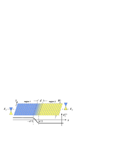
The setup of our simulation is illustrated in Fig. 1. A graphene strip of width $W$ is divided into two regions by a transition area with length $d$. In either region the carrier type and density can be locally tuned through an electrostatic gating, and the relative value of the Fermi energy to the local charge neutrality point is defined as the relative Fermi energy $E_{f}^{(r)}$. The whole sample is subject to a perpendicular magnetic field, and the Landau levels are formed in the quantum Hall regime.Gusynin05prl With a specific Fermi energy, the filling factor of Landau levels is scarcely dependent on the details of the sample edge, provided the sample size is big enough,note1 therefore we use samples with zigzag edges to carry out our simulation but the results are applicable to general cases. On the energy scale of our problem, both Zeeman splitting and spin-orbit interaction are negligibly small, different spin states can be taken as degenerate and uncorrelated, thus we assume spin is irrelevant in our calculation and simply multiply the result by a factor accounting for the spin degree of freedom. For this reason the filling factors $\nu_{1}$ and $\nu_{2}$ given below are all ”spinless”, i.e., their values are $\pm 1$, $\pm 3$, $\pm 5\cdots$ instead of $\pm 2$, $\pm 6$, $\pm 10\cdots$.

Magneto-conductance of a graphene p-n junction has been theoretically discussed in terms of its valley isospin dependence.GPNJtheories These discussions in general assume an absence of intervalley scattering across the graphene p-n junction. To explain the fractionally quantized plateaus observed in the experiments,Williams07sci ; Ozyilmaz07prl however, full mode mixing was required in random matrix theory, which inevitably involves intervalley scatteringAbanin07sci . We attribute the inter-valley scattering in our model to disorder potential which varies quickly enough in the scale of the lattice constant. Disorder in graphene may have various sources, and the understanding of its role in transport properties is still incomplete.Neto07091163 ; Pereira08prb

In this paper we focus on the effect of the random potential at the interface of the junction. The reason is that current inside either region 1 or region 2 is carried by quantum Hall edge states,Brey06prb thus immune to most disorder inside either region, while scattering among states at the interface of the two regions contributes to the major effect of disorder on the overall conductance. Disorder at the interface may come from intrinsic sources like vacancies and impurities, or from extrinsic sources like random potential introduced by the irregularities of the gate edge. We model the disorder potential at the interface by using the Anderson-type on-site energyAnderson58 which varies randomly from site to site within the transition area, where a potential slope connecting two sides of the junction serves as the background potential. Hence the total Hamiltonian reads

$$H=\sum\limits_{i}\varepsilon(\bm{r}_{i})c_{i}^{\dagger}c_{i}-\sum\limits_{\langle i,j\rangle}[te^{i\phi_{ij}}c_{i}^{\dagger}c_{j}+h.c.]$$ (1)

where $c_{i}^{\dagger}$ and $c_{i}$ are the electron creation and annihilation operators at site $\bm{r}_{i}\equiv(x_{i},y_{i})$, respectively, $t\approx 2.8$ eV is the nearest neighbor hopping energy in the graphene lattice and $\langle i,j\rangle$ stands for a nearest-neighboring pair,

$$\phi_{ij}=\frac{e}{\hbar}\bm{A}(\frac{\bm{r}_{i}+\bm{r}_{j}}{2})\cdot(\bm{r}_{i}-\bm{r}_{j})$$ (2)

is the phase acquired when an electron hopping from $\bm{r}_{j}$ to $\bm{r}_{i}$ in an external field B described by vector potential $\bm{A}$, and the on-site energy $\varepsilon(\bm{r}_{i})$ are $\varepsilon_{1}$ and $\varepsilon_{2}$ in region 1 and 2, respectively;

$$\varepsilon(\bm{r}_{i})=(\varepsilon_{2}-\varepsilon_{1})\frac{x_{i}}{d}+\frac{1}{2}(\varepsilon_{1}+\varepsilon_{2})+\mbox{rand}(\Delta)$$ (3)

in the transition area ($|x_{i}|\leq d/2$) with rand$(\Delta)$ a random number uniformly distributed in $[-\Delta/2,\Delta/2]$. The width of the junction in our simulation is taken to be $W=200(\sqrt{3}a/2)\approx 42.6$ nm, where $a\approx 0.246$ nm is the lattice constant of graphene, and the length of the interface area is taken to be $d=20a\approx 4.9$ nm. Landau gauge $\bm{A}(\bm{r})=(-By,0)$ is adopted, with the magnitude of the magnetic field $B\approx 113$ Tesla which is equivalent to a magnetic flux $\Phi=h/701e$ in each unit cell. The magnetic length in this case is $l_{B}=\sqrt{\hbar/(eB)}\approx 2.4$ nm, which is about a half of the length of the interface area, or $1/18$ of the width of the sample. It should be mentioned here that in a real sample which is presumably much larger in size, the magnetic field necessary for the quantum Hall effect can be much smaller.

Figure 2: (Color online) (a) The mean and (b) the variance of the transmission function $T$ as functions of the relative Fermi energy $E_{f}^{(r2)}$ in region 2, with fixed relative Fermi energy $E_{f}^{(r1)}$ in region 1 and fixed disorder strength $\Delta$. Cases with different $E_{f}^{(r1)}$ and different $\Delta$ are also compared. $E_{f}^{(r1)}>0$ implies n-type of region 1, $E_{f}^{(r1)}/t=0.10$ corresponds to the filling factor $\nu_{1}=1$ and $E_{f}^{(r1)}/t=0.15$ corresponds to $\nu_{1}=3$.

We assume coherent transport in the graphene junction, where the Landauer-Büttiker formalism can be applied.LB Transmission functions $T_{pq}$ ($p,q=1,2$ and $p\neq q$) of the junction are calculated by using the recursive Green’s function technique.Lee81prl ; Li Vanishing net current in equilibrium implies that $T_{21}=T_{12}=T$, therefore the conductance is proportional to either of the transmission functions, $G=(e^{2}/{h})T$, where the spin degeneracy has been included in $T$, and the variance of the conductance $\mbox{Var}(G)=(e^{2}/{h})^{2}\mbox{Var}(T)$, where $\mbox{Var}(T)$ represents the variance of $T$. In the following we will be satisfied with observing only the behavior of $T$ in different situations. Each situation, that is, each experimental condition under which measurements are made, is identified with a specified combination of $\varepsilon_{1}$, $\varepsilon_{2}$ and $\Delta$, while various configurations of disorder are subject to some self-averaging process in each measurement. This self-averaging process could be a result of time dependent electric field used in the experiments,Abanin07sci and will suppress the fluctuation of the measured conductance, thus makes the mean value a reasonable account for the experimental observation. Our calculation extracts the mean and the variance of the transmission functions $T$ in each situation from output of 40,000 samples with different disorder configurations.

III Results

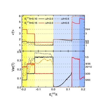
The calculated transmission functions as shown in Fig. 2(a) have surprisingly recovered the quantized transport plateaus observed in the experiment by Williams et al.Williams07sci In junctions with the disorder strength $\Delta=2t$ (solid lines in Fig. 2), the ensemble average of the transmission functions form nearly perfect plateaus in the bipolar regime ($E_{f}^{(r2)}<0$), and the height of each plateau is

$$\langle T\rangle=2\times\frac{|\nu_{1}\nu_{2}|}{|\nu_{1}|+|\nu_{2}|}$$ (4)

with $\nu_{\mbox{\scriptsize total}}\equiv|\nu_{1}|+|\nu_{2}|$. Corresponding to each plateau of the averaged transmission function, the ensemble variance of $T$ also develops into a plateau described by

$$\mbox{Var}(T)=4\times\frac{(\nu_{1}\nu_{2})^{2}}{\left(|\nu_{1}|+|\nu_{2}|\right)^{2}[(|\nu_{1}|+|\nu_{2}|)^{2}-1]}.$$ (5)

Both Eq. (4) and Eq. (5) are the predictions of the RMT on a quantum chaotic cavity,Beenakker97rmp with the additional factors 2 and 4 from the spin degeneracy. In the unipolar regime ($E_{f}^{(r2)}>0$), plateaus of the ensemble average $\langle T\rangle$ are only partly formed when $\Delta=2t$, and the height may not be accurately of the expected values given by

$$\langle T\rangle=2\times\mbox{min}(|\nu_{1}|,|\nu_{2}|)$$ (6)

The transmission functions show large ensemble variance where $\langle T\rangle$ has a large deviation from Eq. (6). Decreased disorder strength in the junction interface, in contrast, leads to better-developed plateaus of $\langle T\rangle$ in the unipolar regime, at the cost of losing the quantized values of $\langle T\rangle$ and Var($T$) in the bipolar regime. This is presented as the dash lines in Fig. 2 with $\Delta=0.5t$.

The plateaus described by Eq. (4) in the bipolar regime and described by Eq. (6) in the unipolar regime are the signature of the quantum Hall effect in a single graphene junction,Williams07sci though in some cases the accuracy of the plateau is poor in the experimental data,Williams07sci ; Ozyilmaz07prl compared with the expected value. By taking into account disorder in the junction interface area and a self-averaging process in the measurement, our calculations clearly produce these plateaus. In addition, the lack of the accuracy of the plateau height is attached to the strength of the disorder, and is reflected in the variance of the transmission functions.

Figure 3: (Color online) (a) The mean and (b) the variance of the transmission function $T$ as functions of the disorder strength $\Delta$ in bipolar junctions. Region 1 is of n-type with the filling factor $\nu_{1}=1$, and region 2 is of p-type with the filling factor $\nu_{2}=-1,-3,-5$, respectively. The shadow highlights the regime where both $\langle T\rangle$ and Var($T$) show plateaus predicted by Eq. (4) and Eq. (5), respectively.

The experimentally observed conductance plateaus of a bipolar graphene junction in the quantum Hall regime have been explained as the result of the complete mixing of quantum Hall edge states at the junction interface due to scattering, and the departures of the experimental data from Eq. (4) have been attributed to the incomplete mixing of edge states.Williams07sci ; Abanin07sci We emphasize here that because the spin-flip process is negligible in this system, the mode mixing can only happen among states of the same spin quantum number. Thus to correctly express $\langle T\rangle$ and Var($T$) in terms of the filling factors $\nu_{1}$ and $\nu_{2}$, the filling factors must be spinless, with the spin degree of freedom included as an extra multiplier to $T$. Such expressions, compared with the expressions using the spinful filling factors $\pm 2$, $\pm 6$, $\pm 10$…,Abanin07sci show no quantitative difference as for $\langle T\rangle$, but significant differences as for Var($T$).

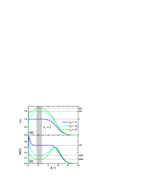
The disorder dependence of the transmission functions with specific combinations of filling factors in the bipolar regime is shown in Fig. 3. The shadowed region (roughly $1.7t<\Delta<2.8t$) is where complete mode mixing happens in all three cases, i.e. $\nu_{1}=1$ and $\nu_{2}=-1,-3,-5$, respectively. The averaged transmission functions develop into plateaus of height described by Eq. (4) simultaneously in this region, and the ensemble variances of the transmission functions also develop into plateaus predicted by Eq. (5). In the language of the RMT,BarangerJalabert94 ; Beenakker97rmp the ensembles of scattering matrices $S$ (of a specific spin quantum number) under these circumstances are the circular unitary ensembles (CUEs), that is, $S$ matrices in these ensembles are uniformly distributed over the unitary group $\mathcal{U}(\nu_{\mbox{\scriptsize total}})$. Average over the CUE is equal to an integration over the unitary group. And it is this integration that lead to the ”universal” value of the averaged transmission function Eq. (4), and the universal conductance fluctuation (UCF) given by Eq. (5). The graphene bipolar junctions in this disorder regime (shadowed) are nearly ideal realizations of the quantum chaotic cavities characterized by Eq. (4) and (5).

The ensemble of $S$ matrices, however, is actually dependent on the disorder strength $\Delta$, which represents how much the scattering potential can be varied from one sample to another. In Fig. 3 we see that to the left of the shadowed region (roughly $\Delta<1.7t$), both $\langle T\rangle$ and Var($T$) deviate from Eq. (4) and (5) with decreased $\Delta$, indicating the deviation of the actual ensembles of $S$ matrices from the CUEs. In other words, these are the cases of incomplete mode mixing. Notably, when $\nu_{1}=-\nu_{2}=1$ there is an extended range of $\Delta$ where the plateau of $\langle T\rangle$ is preserved. This is easily understood as there are only two modes to be mixed in this case. When the disorder at the junction interface is larger than the range of the shadowed region in Fig. 3, on the other hand, the conducting edge modes in either region 1 or region 2 are expelled from the junction interface area gradually, scattering between modes from one side of the junction to the other is weak, both $\langle T\rangle$ and Var($T$) decrease until the whole junction is ”cut off”. This is the case of what we see in the large-$\Delta$ regime of Fig. 3.

Figure 4: (Color online) The averaged transmission function $\langle T\rangle$ as a function of the disorder strength $\Delta$ in unipolar (n-n) junctions with different combinations of filling factors. The inset shows the corresponding variance of $T$. The regime is shadowed where all plateaus of $\langle T\rangle$ are preserved.

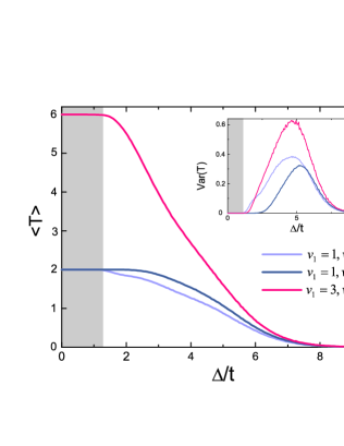
Compared with the bipolar junctions, transport in a unipolar junction with disordered junction interface has a more straightforward picture. The conductance of a unipolar junction is mainly contributed from the compatible edge modes in the two regions, and the tunneling of carriers from one region to another mainly happens near the lateral edges. The disorder at the interface impedes the coupling of these modes to reduce the transmission through the junction, which is contrary to the bipolar cases. The calculated $\langle T\rangle$ and Var($T$) in the unipolar regime are shown in Fig. 4 with different combinations of filling factors. In each case $\langle T\rangle$ exhibits a quantized plateau when the disorder is weak (shadowed), and starts to deviate from the plateau at a critical value of the disorder strength where Var($T$) also begins to deviate from zero. We notice that the shadowed regions in Fig. 3 and 4 do not overlap over the range of $\Delta$, which implies that $\langle T\rangle$ do not develop into plateaus simultaneously in the bipolar regime and the unipolar regime, especially when the filling factors are large. This fact highlights the opposite roles the disorder plays in the formation of conductance plateaus in the bipolar and the unipolar junctions. It stabilizes the plateaus in the bipolar case when its intensity is in a certain nonzero range, while it tends to destroy the plateaus in the unipolar case at the same time, though in the limit of strong disorder electrons will be blocked from tunneling through the junction in both cases.

Figure 5: (Color online) The Fano factors in the bipolar regime, as functions of the relative Fermi energy $E_{f}^{(r2)}$, with $\nu_{1}$ = 1 (black) and 3 (red/dark gray), respectively, and $\Delta=2t$. Plateaus predicted by Eq. (7) are indicated by short dash lines.

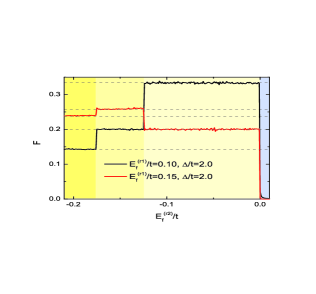
The character of the quantized transport in these junctions can be experimentally identified by measuring the electron shot noise.Blanter00 The Fano factor, defined as the ratio of the actual shot noise to the Poisson noise, is extracted from our simulation using the equation $F=\langle\sum T_{n}(1-T_{n})\rangle/\langle\sum T_{n}\rangle$, where the summations are taken over different transmission eigenvalues indexed by $n$. It is found that the Fano factors corresponding to the conductance plateaus in the unipolar regime are identically zero, as expected from the dissipationless transport via the quantum Hall edge modes. In the bipolar regime, the Fano factors develop into plateaus described by

$$F=\frac{|\nu_{1}\nu_{2}|}{\left(|\nu_{1}|+|\nu_{2}|\right)^{2}-1}$$ (7)

corresponding to the plateaus of $\langle T\rangle$, as shown in Fig. 5. Eq. (7) is again a straightforward outcome of the RMT applied to a quantum chaotic cavity with few transmission modes.Savin06 It is quantitatively different from the Fano factors discussed in reference Abanin07sci , especially when the number of the transmission modes is small. And this is a key to examine experimentally the existence of the UCF revealed in our simulation.

IV Discussions and conclusion

Before ending this paper we address the issues on the sources and types of disorder in graphene which is relevant to this study. The experimentally observed conductance plateaus were explained as a result of the full mixing of these quantum Hall edge modes.Williams07sci ; Abanin07sci The details of the mode mixing are determined by the form of the disorder and in turn provide information about the disorder therein. The quantum Hall edge modes in a graphene strip can be indexed by two quantum numbers, spin and valley isospin,Akhmerov07prl besides the Landau levels they belong to. Thus the mechanism of the mode mixing inevitably involves the presence of spin-flip scattering and/or intervalley scattering. Considering the negligible magnetic impurities and spin-related interaction in the current graphene samples, and ignoring the magnetic edge states reported in some specific graphene ribbons,Son06nat , we assume the absence of spin-flip scattering in this study, and use the ”spinless” filling factors $\nu_{1}$ and $\nu_{2}$ ($=\pm 1,\pm 3,\pm 5\cdots$) in our expressions.note2 The presence of intervalley scattering among the quantum Hall edge modes in the graphene p-n junctions, however, is still a question. Previous works on the disorder effects in graphene p-n junctions generally assumed weak intervalley scattering, and discussed the valley-isospin dependence of the conductance.GPNJtheories For example, in the work by Tworzydło et al.,Tworzydlo07prb it was assumed that each impurity has the Gaussian potential profile $U_{i}\exp(-|\bm{r}-\bm{R}_{i}|^{2}/2\xi^{2})$ of range $\xi$ and random height $U_{i}\in(-\delta,\delta)$. A large $\xi$ implies a long range of the disorder potential which suppresses the intervalley scattering, while a small $\xi$ implies $\delta$-function-like disorder potential which provokes the intervalley scattering. The former case was studied but the plateaus observed in the experiments were not properly recovered. That is the reason why we choose the latter case as our starting point in this work, though the origin of the short-range disorder potential is not completely understood. It turns out our calculations do produce the reported conductance plateaus as in Eq. (4), as well as quantities like the Fano factors as in Eq. (7) that can be further examined experimentally. Still it is interesting to investigate the crossover effects between long-range disorder potential and short-range disorder potential in the junctions, and the results would possibly explain the not-fully-developed conductance plateaus in the experiments.Williams07sci ; Ozyilmaz07prl This investigation will be a subject of our later work. Furthermore, there also exist other forms of disorder that cannot be described by random local potential,Neto07091163 ; Pereira08prb . For example, effective gauge fields can be induced by ripples, topological lattice defects, strains, or curvatures etc. in the graphene sample, and will affect the Landau levels, especially the lowest one.Guinea08prb We believe that these various forms of disorder will affect the behavior of the edge-mode mixing in various manners, but this is out of the scope of the current work.

In short, our numerical simulation of the quantum Hall effect in graphene p-n junctions has reproduced the quantized conductance plateaus observed in the experiment. The UCF and quantized values of the Fano factors are found to be accompanying the conductance plateaus in the bipolar regime, which is well explained by the RMT of quantum transport. The bipolar graphene junction in the quantum Hall regime mimics an ideal quantum chaotic cavity, which is another example of the extraordinary transport character of graphene.

V Appendix: Derivation of Eqs. (4), (5), and (7)

In this appendix, we derive Eqs. (4), (5), and (7) using the random matrix theory.

Random matrix theory of quantum transport is based on the assumption that the scattering matrix $S$ of a chaotic cavity is uniformly distributed over a specific group (the so-called circular ensemble) determined by the symmetry of the Hamiltonian. Basically there are three classes of the groups.Dyson1962 If time-reversal symmetry is broken ($\beta=2$), $S$ is only constrained by unitarity, which is a result of current conservation, thus $S$ belongs to a unitary group. If time-reversal symmetry is preserved together with the presence of spin-rotation symmetry ($\beta=1$), then $S$ is both unitary and symmetric: $S=S^{T}$, where the superscript $T$ indicates the transpose of the matrix, this leads to an orthogonal group. If time-reversal symmetry is preserved but spin-rotation symmetry is broken ($\beta=4$), which is the case when spin-orbit interaction is present, then $S$ is unitary and self-dual: $S=S^{R}$, where the superscript $R$ indicates the dual of a quaternion matrix, the group is called symplectic.

In random matrix theory, the statistics of transport properties is obtained from the statistics of an appropriate circular ensemble. For example, the mean of the transmission probability $T_{nm}\equiv|S_{nm}|^{2}$ is given by

$$\langle T_{nm}\rangle=\int d\mu(S)S_{nm}S_{nm}^{\ast}$$ (8)

where $n$ and $m$ stand for transmission eigen-channels. We will omit the mathematical details of formulating the measure $d\mu(S)$ in a group space that $S$ belongs to, and use the following two equations as being established:math

$$\langle U_{\alpha a}U_{\beta b}^{\ast}\rangle_{\mbox{\scriptsize CUE}}=\frac{1}{N}\delta_{\alpha\beta}\delta_{ab}$$ (9)

$$\langle U_{\alpha a}U_{\alpha^{\prime}a^{\prime}}U_{\beta b}^{\ast}U_{\beta^{\prime}b^{\prime}}^{\ast}\rangle_{\mbox{\scriptsize CUE}}$$

$$= \frac{1}{N^{2}-1}(\delta_{\alpha\beta}\delta_{ab}\delta_{\alpha^{\prime}\beta^{\prime}}\delta_{a^{\prime}b^{\prime}}+\delta_{\alpha\beta^{\prime}}\delta_{ab^{\prime}}\delta_{\alpha^{\prime}\beta}\delta_{a^{\prime}b})$$

$$- \frac{1}{N(N^{2}-1)}(\delta_{\alpha\beta}\delta_{ab^{\prime}}\delta_{\alpha^{\prime}\beta^{\prime}}\delta_{a^{\prime}b}+\delta_{\alpha\beta^{\prime}}\delta_{ab}\delta_{\alpha^{\prime}\beta}\delta_{a^{\prime}b^{\prime}})$$ (10)

where $U$ is an $N$$\times$$N$ unitary matrix belonging to the circular unitary ensemble (CUE). Since the system we are going to discuss only involves the CUE, we will drop this notation hereafter.

Starting from these equations, the conductance $\langle G\rangle$, its fluctuation Var($G$), and the Fano factor $F$ for the fully-mixed quantum hall edge transport in a graphene p-n junction can be readily calculated. We first assume no spin-flip scattering is allowed, so that $S$ matrix for each spin component is unitary by itself, the case including spin-flip scattering will be discussed in what follows. Suppose there are $2$$N_{1}$ and $2$$N_{2}$ edge states (they are also eigen-channels away from the junction area) at the two sides of the junction, respectively, the full $S$ matrix is of dimension $2(N_{1}+N_{2})$, but it is divided into two uncoupled spin subspaces in the absence of spin-flip scattering, therefore matrices in the CUE are only of dimension $N_{\mbox{\scriptsize total}}=N_{1}+N_{2}$ in terms of each spin subspace. Also the strict spin degeneracy implies that $S_{nm}^{\sigma}=S_{nm}^{-\sigma}=S_{nm}$. Regarding this we have

$$\langle G\rangle = \sum\limits_{\sigma=\pm 1}\sum\limits_{n=1}^{N_{1}}\sum\limits_{m=1}^{N_{2}}\langle T_{nm}^{\sigma}\rangle\frac{e^{2}}{h}$$ (11)

$$= \>2\sum\limits_{n=1}^{N_{1}}\sum\limits_{m=1}^{N_{2}}\langle S_{nm}S^{*}_{nm}\rangle\frac{e^{2}}{h}$$

$$= \frac{2N_{1}N_{2}}{N_{1}+N_{2}}\frac{e^{2}}{h},$$

$$\mbox{Var}(G) =(\langle G^{2}\rangle-\langle G\rangle^{2}$$

$$= \left\langle\left(\sum\limits_{\sigma=\pm 1}\sum\limits_{n=1}^{N_{1}}\sum\limits_{m=1}^{N_{2}}T_{nm}^{\sigma}\right)^{2}\right\rangle\left(\frac{e^{2}}{h}\right)^{2}-\langle G\rangle^{2}$$

$$= 4\sum\limits_{n,n^{\prime}=1}^{N_{1}}\sum\limits_{m,m^{\prime}=1}^{N_{2}}\langle S_{nm}S_{n^{\prime}m^{\prime}}S_{nm}^{*}S_{n^{\prime}m^{\prime}}^{*}\rangle\left(\frac{e^{2}}{h}\right)^{2}-\langle G\rangle^{2}$$

$$= \frac{4N_{1}^{2}N_{2}^{2}}{\left(N_{1}+N_{2}\right)^{2}\left[(N_{1}+N_{2})^{2}-1\right]}\left(\frac{e^{2}}{h}\right)^{2}.$$ (12)

The Fano factor $F=\langle\mbox{Trace}(tt^{\dagger}(1-tt^{\dagger}))\rangle/\langle\mbox{Trace}(tt^{\dagger})\rangle$, where $t$ is the transmission submatrix of $S$,lastnote and $\mbox{Trace}(tt^{\dagger})$ is nothing but $G/\frac{e^{2}}{h}$. Thus

$$F= 1-\frac{N_{1}+N_{2}}{2N_{1}N_{2}}\sum\limits_{\sigma=\pm 1}\sum\limits_{n,n^{\prime}=1}^{N_{1}}\sum\limits_{m,m^{\prime}=1}^{N_{2}}\langle S_{nm}^{\sigma}S_{n^{\prime}m}^{\sigma\;\ast}S_{n^{\prime}m^{\prime}}^{\sigma}S_{nm^{\prime}}^{\sigma\;\ast}\rangle$$

$$= \frac{N_{1}N_{2}}{\left(N_{1}+N_{2}\right)^{2}-1}$$ (13)

In this way we have derived the formulae expressed in Eqs. (4), (5), and (7) in the framework of the random matrix theory.

In contrast to the spin-conserved scattering case, the mixing among different spin modes will lead to quantitatively different variance and Fano factors, while leaving the conductance mean unchanged. In the random matrix theory, this is derived as following. Still suppose there are $2$$N_{1}$ and $2$$N_{2}$ edge states at the two sides of the junction respectively, the full $S$ matrix is still of dimension $2(N_{1}+N_{2})$, but the spin-off-diagonal parts are now non-zero, and the $S$ matrix is unitary only as a whole. It is straightforward to show that in this case the formulae corresponding of Eqs. (4), (5), and (7) are given by

$$\langle G\rangle = \frac{4N_{1}N_{2}}{2N_{1}+2N_{2}}\frac{e^{2}}{h}$$ (14)

$$= \frac{2N_{1}N_{2}}{N_{1}+N_{2}}\frac{e^{2}}{h},$$

$$\mbox{Var}(G) = \frac{(4N_{1}N_{2})^{2}}{\left(2N_{1}+2N_{2}\right)^{2}[(2N_{1}+2N_{2})^{2}-1]}\left(\frac{e^{2}}{h}\right)^{2}$$ (15)

$$= \frac{4N_{1}^{2}N_{2}^{2}}{\left(N_{1}+N_{2}\right)^{2}[(N_{1}+N_{2})^{2}-1/4]}\left(\frac{e^{2}}{h}\right)^{2},$$

and

$$F = \frac{4N_{1}N_{2}}{\left(2N_{1}+2N_{2}\right)^{2}-1}$$ (16)

$$= \frac{N_{1}N_{2}}{\left(N_{1}+N_{2}\right)^{2}-1/4},$$

respectively. Except for a coincident equivalence of the mean values of the conductance $\langle G\rangle$, the quantitative differences of the UCF $\mbox{Var}(G)$ and the Fano factors $F$ between two cases, namely whether scattering is spin-conserved or not, are obvious, especially when the values of $N_{1}$ and $N_{2}$ are small.

References

- (1) K. S. Novoselov, A. K. Geim, S. V. Morozov, D. Jiang, Y. Zhang, S. V. Dubonos, I. V. Grigorieva, and A. A. Firsov, Science 306, 666 (2004); K. S. Novoselov, D. Jiang, F. Schedin, T. J. Booth, V. V. Khotkevich, S. M. Morozov, and A. K. Geim, Proc. Natl. Acad. Sci. 102, 10451 (2005).
- (2) A. K. Geim and K. S. Novoselov, Nat. Mater. 6, 183 (2007).
- (3) M. I. Katsnelson and K. S. Novoselov, Solid State Commun. 143, 3 (2007).
- (4) A. H. Castro Neto, F. Guinea, N. M. R. Peres, K. S. Novoselov, and A. K. Geim, arXiv:0709.1163.
- (5) K. S. Novoselov, A. K. Geim, S. V. Morozov, D. Jiang, M. I. Katsnelson, I. V. Grigorieva, S. V. Dubonos, and A. A. Firsov, Nature 438, 197 (2005).
- (6) Y. B. Zhang, Y. W. Tan, H. L. Stormer, and P. Kim, Nature 438, 201 (2005).
- (7) J. R. Williams, L. DiCarlo, and C. M. Marcus, Science 317, 638 (2007).
- (8) B. Özyilmaz, P. Jarillo-Herrero, D. Efetov, D. A. Abanin, L. S. Levitov, and P. Kim, Phys. Rev. Lett. 99, 166804 (2007).
- (9) D. A. Abanin and L. S. Levitov, Science 317, 641 (2007).
- (10) R. Landauer, IBM J. Res. Dev. 1, 223 (1957); R. Landauer, Phil. Mag. 21, 863 (1970); M. Büttiker, IBM J. Res. Dev. 32, 317 (1988); M. Büttiker, Phys. Rev. B 38, 9375 (1988).
- (11) H. U. Baranger and P. A. Mello, Phys. Rev. Lett. 73, 142 (1994); R. A. Jalabert, J. L. Pichard, and C. W. J. Beenakker, Europhys. Lett. 27, 255 (1994).
- (12) C. W. J. Beenakker, Rev. Mod. Phys. 69, 731 (1997).
- (13) V. P. Gusynin and S. G. Sharapov, Phys. Rev. Lett. 95, 146801 (2005).
- (14) See, for instance, Fig. 21 in the review by Neto et al.Neto07091163 .
- (15) V. V. Cheianov and V. I. Fal’ko, Phys. Rev. B 74, 041403(R) (2006); J. Tworzydło, I. Snyman, A. R. Akhmerov, and C. W. J. Beenakker, Phys. Rev. B 76, 035411 (2007); A. V. Shytov, Nan Gu, and L. S. Levitov, arXiv:0708.3081 (unpublished).
- (16) Vitor M. Pereira, J. M. B. Lopes dos Santos, and A. H. Castro Neto, Phys. Rev. B 77, 115109 (2008).
- (17) L. Brey and H. A. Fertig, Phys. Rev. B 73, 195408 (2006).
- (18) P. W. Anderson, Phys. Rev. 109, 1492 (1958).
- (19) P. A. Lee and D. S. Fisher, Phys. Rev. Lett. 47, 882 (1981).
- (20) J. Li, L. B. Hu, and S. Q. Shen, Phys. Rev. B 71, 241305(R)(2005) ; J. Li and S. Q. Shen, Phys. Rev. B 76, 153302 (2007)
- (21) Y. M. Blanter and M. Buttiker, Phys. Rep. 336, 1 (2000).
- (22) D. V. Savin and H. J. Sommers, Phys. Rev. B 73, 081307(R) (2006).
- (23) A. R. Akhmerov and C. W. Beenakker, Phys. Rev. Lett. 98, 157003 (2007).
- (24) Y. W. Son, M. L. Cohen, and S. G. Louie, Nature 444, 347 (2006).
- (25) By the random matrix theory, the calculations including or excluding mixing of different spin modes lead to the same expression for the averaged conductance, but different expressions for the conductance fluctuation and the Fano factor, which is derived in the Appendix. And this accounts for the differences between Eqs. (5) and (7) in this work and Eqs. (4) and (10) in the work by Abanin and Levitov.Abanin07sci
- (26) J. Tworzydło, I. Snyman, A. R. Akhmerov, and C. W. J. Beenakker, Phys. Rev. B 76, 035411 (2007).
- (27) F. Guinea, B. Horovitz, and P. L. Doussal, Phys. Rev. B 77, 205421 (2008)
- (28) F. J. Dyson, J. Math. Phys. (N.Y.) 3, 1199 (1962).
- (29) M. Creutz, J. Math. Phys. (N.Y.) 19, 2043 (1978); S. Samuel, J. Math. Phys. (N.Y.) 21, 2695 (1980).
-
(30)
In general can be written in terms of its transmission
and reflection parts as
- (31) W. Long, Q. F. Sun, and J. Wang, arXiv: 0807.1578