Electric Dipole Moments in U(1)^′ Models

Abstract

We study electric dipole moments (EDM) of electron and proton in E(6)–inspired supersymmetric models with an extra U(1) invariance. Compared to the Minimal Supersymmetric Standard Model (MSSM), in addition to offering a natural solution to the $\mu$ problem and predicting a larger mass for the lightest Higgs boson, these models are found to yield suppressed EDMs.

I Introduction

While solving the quadratic divergence of radiative corrections to the Higgs boson mass, the supersymmetrization of the Standard Model with minimal matter content brings a $\mu$ parameter with a completely unknown scale. On the other hand, extending the gauge structure $SU(3)_{C}\times SU(2)_{L}\times U(1)_{Y}$ of the Minimal Supersymmetric Model by a new $U(1)$ Abelian group provides an effective $\mu$ term related with the VEV of some extra singlet scalar field; thus a scale ($\sim TeV$) can be dynamically generated for the $\mu$ parameter. The supersymmetric $U(1)^{\prime}$ models have been intensely studied in the literature. While such models can be motivated by low-energy arguments like $\mu$ problem muprob of the MSSM they also arise at low-energies as remnants of GUTs such as $SO(10)$ and $E(6)$ Robinett:1981yz ; Robinett:1982tq ; Langacker:1984dc . These models necessarily involve an extra neutral vector boson Cvetic:1995rj ; Cvetic:1996mf whose absence/presence to be established at the LHC.

The particle spectrum of $U(1)^{\prime}$ models involve bosonic fields $Z_{\mu}^{\prime}$ and $S$ as well as their superpartners $\widetilde{Z}^{\prime}$ and $\widetilde{S}$ in addition to those in the MSSM. Therefore, such models can be tested in various observables ranging from electroweak precision observables to $Z_{\mu}^{\prime}$ effects at the LHC. As a matter of fact, analysis of Higgs sector along with CP violation potential Demir:2005kg as well as structure of EDMs Suematsu:1998wm suggest several interesting signatures also at collider experiments King:2005jy . One of the most important spots of these models is that the lower bound of the lightest Higgs boson mass ($m_{h}\geq$114 GeV) can be satisfied already at the tree level, and radiative corrections (dominantly the top–stop mass splitting) is not needed to be as large as in the MSSM. This feature can have important implications also for the little hierarchy problem Demir:2005ti .

In this work we will study EDMs of electron and neutron in $U(1)^{\prime}$ models stemming from $E(6)$ GUT. Our main interest is to look at the reaction of EDMs to gauge extensions in comparison to the MSSM. The paper is organized as follows. In the next section we introduce the models. Section III is devoted to EDM predictions and their numerical analysis. In Section IV we conclude.

II The $U(1)^{\prime}$ Models

The model is characterized by the gauge structure

$$SU(3)_{C}\times SU(2)_{L}\times U(1)_{Y}\times U(1)_{Y^{\prime}}$$ (1)

where $g_{3}$, $g_{2}$, $g_{Y}$ and $g_{Y^{\prime}}$ are gauge coupling constants respectively. Here the extra $U(1)$ symmetry can be a light (broken at a $\rm{TeV}$) linear combination of a number of U(1) symmetries (in effective string models there are several U(1) factors whose at least one combination can survive down to the $\rm{TeV}$ scale). There are a number of $U(1)^{\prime}$ models studied in literature, all of them offer a dynamical solution to the $\mu$ problem of the MSSM via spontaneous breaking of extra $U(1)$ Abelian factor at the $\rm{TeV}$ scale depending on the model, and many of them respecting gauge couplings unification predicts extra fields in order to sort out gauge and gravitational anomalies from the theory. These models typically arise from SUSY GUTs and strings. From $E(6)$ GUT, for example, two extra $U(1)$ symmetries appear in the breaking $E6\rightarrow SO(10)\times U(1)_{\psi}$ followed by $SO(10)\rightarrow SU(5)\times U(1)_{\chi}$ where $U(1)_{Y^{\prime}}$ is a linear combination of $\psi$ and $\chi$ symmetries:

$$U(1)_{Y^{\prime}}=\cos{\theta_{E6}}\,U(1)_{\chi}-\sin{\theta_{E6}}\,U(1)_{\psi}$$ (2)

which, supposedly, is broken spontaneously at a ${\rm TeV}$. There arises, in fact, a continuum of $U(1)^{\prime}$ models depending on the value of mixing angle $\theta_{E_{6}}$. However, for convenience and traditional reasons, one can pick up specific values of $\theta_{E_{6}}$ to form a set of models serving a testing ground. We thus collected some well-known models in Table 1 with the relevant normalization factors and a common gauge coupling constant

$$g_{Y^{\prime}}=\sqrt{\frac{5}{3}}g_{2}\tan{\theta_{W}}$$ (3)

	$2\sqrt{15}~{}Q_{\eta}$	$~{}~{}2~{}Q_{I}~{}~{}$	$2\sqrt{6}~{}Q_{\psi}$	$2\sqrt{10}~{}Q_{N}$	$2\sqrt{15}~{}Q_{S}$
$u_{L},d_{L}$	-2	0	1	1	-1/2
$u_{R}$	2	0	-1	-1	1/2
$d_{R}$	-1	1	-1	-2	-4
$e_{L}$	1	-1	1	2	4
$e_{R}$	2	0	-1	-1	1/2
$H_{u}$	4	0	-2	-2	1
$H_{d}$	1	1	-2	-3	-7/2
$S$	-5	-1	4	5	5/2

Table 1: Gauge quantum numbers of several $U(1)^{\prime}$ models Langacker:2008yv

In theories involving more than one $U(1)$ factor the kinetic terms can mix since for such symmetries the field strength tensor itself is invariant. In $U(1)^{\prime}$ model, involving hypercharge $U(1)_{Y}$ and $U(1)_{Y^{\prime}}$, the gauge part of the Lagrangian takes the form

$$-{\cal L}_{gauge}=\frac{1}{4}F_{Y}^{\mu\nu}F_{Y\mu\nu}+\frac{1}{4}F_{Y^{\prime}}^{\mu\nu}F_{Y^{\prime}\mu\nu}+\frac{\sin{\chi}}{2}F_{Y}^{\mu\nu}F_{Y^{\prime}\mu\nu}$$ (4)

where $F_{\mu\nu}=\partial_{\mu}Z_{\nu}-\partial_{\nu}Z_{\mu}$ is the field strength tensor of the corresponding $U(1)$ symmetry. Kinetic part of Lagrangian can be brought into canonical form by a non-unitary transformation

$$\left(\begin{array}[]{c}\hat{W}_{Y}\\ \hat{W}_{Y^{\prime}}\end{array}\right)=\left(\begin{array}[]{c c}1&-\tan{\chi}\\ 0&1/\cos{\chi}\end{array}\right)\left(\begin{array}[]{c}\hat{W}_{B}\\ \hat{W}_{B^{\prime}}\end{array}\right)$$ (11)

where $\hat{W}_{Y}$ and $\hat{W}_{Y^{\prime}}$ are the chiral superfields associated with the two $U(1)$ gauge symmetries. This transformation also acts on the gauge boson and gaugino components of the chiral superfields in the same form. The $U(1)_{Y}\times U(1)_{Y^{\prime}}$ part of covariant derivative in the case of no kinetic mixing is given by

$$D_{\mu}=\partial_{\mu}+ig_{Y}YB_{\mu}+ig_{Y^{\prime}}Q_{Y^{\prime}}B_{\mu}^{\prime}$$ (12)

however, with the presence of kinetic mixing this covariant derivative is changed to

$$D_{\mu}=\partial_{\mu}+ig_{Y}YB_{\mu}+i\left(-g_{Y}Y\tan{\chi}+\frac{g_{Y^{\prime}}}{\cos{\chi}}Q_{Y^{\prime}}\right)B_{\mu}^{\prime}$$ (13)

where $g_{Y^{\prime}}$ is gauge coupling constant and $Q_{Y^{\prime}}$ is fermion charges of $U(1)_{Y^{\prime}}$ symmetry. With a linear transformation of charges the covariant derivative takes the form Choi:2006fz

$$D_{\mu}=\partial_{\mu}+ig_{Y}YB_{\mu}+ig_{Y^{\prime}}Q_{Y^{\prime}}^{\prime}B_{\mu}^{\prime}$$ (14)

in which the effective $U(1)_{Y^{\prime}}$ charges are shifted from its original value $Q_{Y^{\prime}}$ to

$$Q_{Y^{\prime}}^{\prime}=\frac{Q_{Y^{\prime}}}{\cos{\chi}}-\frac{g_{Y}}{g_{Y^{\prime}}}Y\tan{\chi}$$ (15)

For the proper treatment of the models the most general superpotential should be considered King:2005jy , but for simplicity we parametrized $U(1)^{\prime}$ models by the following superpotential

$$\widehat{W}=h_{u}\widehat{Q}\cdot\widehat{H}_{u}\widehat{U^{c}}+h_{d}\widehat{Q}\cdot\widehat{H}_{d}\widehat{D^{c}}+h_{e}\widehat{L}\cdot\widehat{H}_{d}\widehat{E^{c}}+h_{S}\widehat{S}\widehat{H}_{u}\cdot\widehat{H}_{d}$$ (16)

where we discarded additional field (assuming that they are relatively heavy compared to this very spectrum) that are necessary for the unification of gauge couplings. Our conventions are such that, for instance $\widehat{Q}\cdot\widehat{H}_{u}\equiv\widehat{Q}^{T}\left(i\sigma_{2}\right)\widehat{H}_{u}=\epsilon_{ij}\widehat{Q}^{i}\widehat{H}^{j}_{u}$ with $\epsilon_{12}=-\epsilon_{21}=1$. The right-handed fermions are contained in the chiral superfields $\widehat{U}$, $\widehat{D}$, $\widehat{E}$ via their charge-conjugates $e.g.$ $\widehat{U}=\left(\widetilde{u_{R}}^{\star},\left(u_{R}\right)^{C}\right)$. What a $U(1)^{\prime}$ model does is basically to allow a dynamical effective $\mu_{eff}=h_{s}\langle S\rangle$ related to the scale of $U(1)^{\prime}$ breaking instead of an elementary $\mu$ term which troubles supersymmetric Higgsino mass in the MSSM. Notice that a bare $\mu$ term cannot appear in the superpotential due to $U(1)^{\prime}$ invariance.

At this point, it is useful to explicitly state the soft breaking terms, the most general holomorphic structures are

$$-{\mathcal{L}}_{soft} = (\sum_{i}M_{i}\lambda_{i}\lambda_{i}-A_{S}h_{s}SH_{d}H_{u}-A_{u}^{ij}h_{u}^{ij}U^{c}_{j}Q_{i}H_{u}$$ (17)

$$- A_{d}^{ij}h_{d}^{ij}D^{c}_{j}Q_{i}H_{d}-A_{e}^{ij}h_{e}^{ij}E^{c}_{j}L_{i}H_{d}+h.c.)$$

$$+ m_{H_{u}}^{2}|H_{u}|^{2}+m_{H_{d}}^{2}|H_{d}|^{2}+m_{S}^{2}|S|^{2}$$

$$+ m_{Q_{ij}}^{2}\widetilde{Q}_{i}\widetilde{Q}_{j}^{*}+m_{U_{ij}}^{2}\widetilde{U}^{c}_{i}\widetilde{U}^{c*}_{j}+m_{D_{ij}}^{2}\widetilde{D}^{c}_{i}\widetilde{D}^{c*}_{j}+m_{L_{ij}}^{2}\widetilde{L}_{i}\widetilde{L}_{j}^{*}$$

$$+ m_{E_{ij}}^{2}\widetilde{E}^{c}_{i}\widetilde{E}^{c*}_{j}+h.c.$$

where the sfermion mass-squareds $m^{2}_{Q,...,E^{c}}$ and trilinear couplings $A_{u,...,e}$ are $3\times 3$ matrices in flavor space. All these soft masses will be taken here to be diagonal. In general, all gaugino masses, trilinear couplings and flavor-violating entries of the sfermion mass-squared matrices are source of CP violation. However, for simplicity and definiteness we will assume a basis in which entire CP violating effects are confined into the gaugino mass $M_{1}$ (with $M_{1}=M^{\prime}_{1}$), and the rest are all real (interested readers can chief to Demir:2007dt ).

These soft SUSY breaking parameters are generically nonuniversal at low energies. We will not address the origin of these low energy parameters as to how they follow via RG evolution from high energy boundary conditions, instead we will perform a general scan of the parameter space.

III Constraints and Implications for EDMs

Due to the extra $U(1)$ symmetry, associated $Z^{\prime}$ boson can be expected to weigh around the electroweak bosons, and can exhibit significant mixing with the ordinary $Z$ boson. The LEP data and other low-energy observables forbid $Z$–$Z^{\prime}$ mixing to exceed one per mill level. Indeed, precision measurements have shown that $Z^{\prime}$ mass should not be less than $\sim 700$ GeV for any of the models under concern (excluding leptophobic $Z^{\prime}$’s). Indeed, mixing of the $Z$ and $Z^{\prime}$ puts important restrictions on the mass and the mixing angle of the extra boson and this can be studied from the following $Z-Z^{\prime}$ mixing matrix;

$$M_{Z-Z^{\prime}}^{2}=\left(\begin{array}[]{c c}M_{Z}^{2}&\Delta^{2}\\ \Delta^{2}&M_{Z^{\prime}}^{2}\\ \end{array}\right)$$ (20)

with $M_{Z}$ being the usual SM $Z$ mass in the absence of mixing and

$$M_{Z}^{2} = \frac{1}{4}G^{2}(|v_{u}|^{2}+|v_{d}|^{2})$$

$$\Delta^{2} = \frac{1}{2}Gg_{Y^{\prime}}(Q^{\prime}_{H_{u}}|v_{u}|^{2}-Q^{\prime}_{H_{d}}|v_{d}|^{2})$$ (21)

$$M_{Z^{\prime}}^{2} = g_{Y^{\prime}}^{2}({Q^{\prime}}^{2}_{H_{u}}|v_{u}|^{2}+{Q^{\prime}}^{2}_{H_{d}}|v_{d}|^{2}+{Q^{\prime}}^{2}_{s}|v_{S}|^{2})$$

where $G^{2}=g_{Y}^{2}+g_{2}^{2}$ and $g_{Y^{\prime}}$ is the gauge coupling constant of the extra $U(1)$. The mixing matrix can be diagonalized by an orthogonal transformation;

$$\left(\begin{array}[]{c}Z_{1}\\ Z_{2}\end{array}\right)=\left(\begin{array}[]{c c}\cos{\phi}&\sin{\phi}\\ -\sin{\phi}&\cos{\phi}\end{array}\right)\left(\begin{array}[]{c}Z\\ Z^{\prime}\end{array}\right)$$ (28)

giving the mass eigenstates $Z_{1,2}$ with masses $M_{Z_{1},Z_{2}}$ where $\alpha$ is given by

$$\tan{2\alpha}=\frac{2\Delta^{2}}{M_{Z}^{2}-M_{Z^{\prime}}^{2}}$$ (29)

In the numerical analysis we considered $\alpha<3\times 10^{-3}$ and confined $M_{Z^{\prime}}>700$ GeV. Notice that when $\Delta$ vanishes ($\tan{\beta}\sim\sqrt{Q^{\prime}_{H_{u}}/Q^{\prime}_{H_{d}}}$) $Z_{1,2}$ can be identified with the ordinary $Z$ and $Z^{\prime}$ bosons; since we considered low $\tan{\beta}$ values, we will use the term $Z^{\prime}$ for the heavy extra boson.

Besides this, the implication of the extra gauge boson can also be seen in sfermion sector, that is sfermion mass matrix is modified due to the presence of $Z^{\prime}$ boson as;

$${{\cal{M}}}_{\tilde{f}}^{2}=\left(\begin{array}[]{cc}{{\cal{M}}}_{\tilde{f}_{LL}}^{2}&{{\cal{M}}}_{\tilde{f}_{LR}}^{2}\\ {{{\cal{M}}}_{\tilde{f}_{LR}}^{2\star}}&{{\cal{M}}}_{\tilde{f}_{RR}}^{2}\end{array}\right)$$ (32)

$${{\cal{M}}}_{\tilde{f}_{LL}}^{2} = {{\cal{M}}}_{\tilde{f}_{L}}^{2}+h_{f}^{2}|H_{f}^{0}|^{2}+\frac{1}{2}\left(Y_{f_{L}}g_{Y}^{2}-T_{3f}g_{2}^{2}\right)\left(|H_{u}^{0}|^{2}-|H_{d}^{0}|^{2}\right)$$

$$+ g_{Y^{\prime}}^{2}Q_{f_{L}}^{\prime}\left(|H_{u}^{0}|^{2}Q_{H_{u}}^{\prime}+|H_{d}^{0}|^{2}Q_{H_{d}}^{\prime}+|S|^{2}Q_{s}^{\prime}\right)$$

$${{\cal{M}}}_{\tilde{f}_{LR}}^{2} = h_{f}\left(A_{f}^{\star}{H_{f}^{0}}^{\star}+h_{s}SH_{f}^{0}\right)$$ (34)

$${{\cal{M}}}_{\tilde{f}_{RR}}^{2} = {{\cal{M}}}_{\tilde{f}_{R}}^{2}+h_{f}^{2}|H_{f}^{0}|^{2}+\frac{1}{2}\left(Y_{f_{R}}g_{Y}^{2}\right)\left(|H_{u}^{0}|^{2}-|H_{d}^{0}|^{2}\right)$$

$$+ g_{Y^{\prime}}^{2}Q_{f_{R}}^{\prime}\left(|H_{u}^{0}|^{2}Q_{H_{u}}^{\prime}+|H_{d}^{0}|^{2}Q_{H_{d}}^{\prime}+|S|^{2}Q_{s}^{\prime}\right)$$

in terms of shifted charge assignments. Sfermion mass matrix is hermitian and can be diagonalized by the unitary transformation

$$D^{\dagger}{\cal M}_{\tilde{f}}^{2}D=diag(m_{\tilde{f}_{1}}^{2},m_{\tilde{f}_{2}}^{2})$$ (35)

where $D$ is the $L-R$ mixing matrix for sfermions and is parametrized as

$$D=\left(\begin{array}[]{cc}\cos{\theta}&\sin{\theta}\,e^{-i\phi}\\ \sin{\theta}\,e^{i\phi}&\cos{\theta}\\ \end{array}\right)$$ (38)

It is worth to note that sfermion mass eigenvalues in $U(1)^{\prime}$ models will be different than in the MSSM due to the contribution of extra gauge boson and kinetic mixing. In general $D_{U(1)^{\prime}}\neq\,D_{MSSM}$ and the MSSM results can be recovered by assuming no kinetic mixing ($\sin{\chi}=0$) and no charges under $U(1)^{\prime}$ at all.

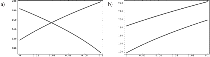
Figure 1: Impact of selectron $U(1)^{\prime}$ charge Q^′ on the selectron masses (In GeVs).

But the existence of the $U(1)^{\prime}$ charges have profound impact on the sfermion eigenvalues. To show this we present Fig. 1 in which selectron mass eigenvalues are plotted against $U(1)^{\prime}$ charges for two different cases. In panel a) we assumed $Q^{\prime}_{eL}=-\,Q^{\prime}_{eR}=Q^{\prime}$ to be compared with panel b) in which $Q^{\prime}_{eL}=Q^{\prime}_{eR}=Q^{\prime}$, with the following inputs: $h_{s}=0.5$, $v_{s}=5$ TeV, $Q^{\prime}_{H_{u}}=Q^{\prime}_{H_{d}}=-0.05$ and the rest of the parameters are taken as in SPS1a^′ reference point AguilarSaavedra:2005pw , and additionally we assumed $A_{s}=A_{t}$. Notice that $Q^{\prime}=0$ corresponds to MSSM prediction. This figure illustrates the difference between the MSSM and of the $U(1)^{\prime}$ sfermion mass predictions, for the same input parameters. As should be inferred from this figure, opposite values of $Q^{\prime}_{fL}$ and $Q^{\prime}_{fR}$ can violate collider bounds for some of the $U(1)^{\prime}$ models while this selection is current for the MSSM, that will be important in the numerical analysis and we will consider somewhat larger values of sfermion gauge eigenstates to overcome this issue.

In $U(1)^{\prime}$ models compared to MSSM, there is an extra single scalar state in Higgs sector, an additional pair of higgsino and gaugino states are covered in neutralino sector and chargino sector is kept structurally unaltered though it is different than the MSSM due to the effective $\mu$ term. Now we will deal with these sectors.

III.1 Higgs Sector

The Higgs sector in $U(1)^{\prime}$ models compared to MSSM is extended by a single scalar state S whose VEV breaks the $U(1)^{\prime}$ symmetry and generates a dynamical $\mu_{eff}=h_{S}\langle S\rangle$. For a detailed analysis of the Higgs sector with CP violating phases we refer to Demir:2003ke and references therein. The tree level Higgs potential gets contributions from F terms, D terms and soft supersymmetry breaking terms:

$$V_{tree}=V_{F}+V_{D}+V_{soft},$$ (39)

in which

$$V_{F} = |h_{s}|^{2}\left[|H_{u}\cdot H_{d}|^{2}+|S|^{2}(|H_{u}|^{2}+|H_{d}|^{2})\right],$$ (40)

$$V_{D} = \frac{G^{2}}{8}\left(|H_{u}|^{2}-|H_{d}|^{2}\right)^{2}+\frac{g_{2}^{2}}{2}(|H_{u}|^{2}|H_{d}|^{2}-|H_{u}\cdot H_{d}|^{2})$$ (41)

$$+ \frac{g_{Y^{\prime}}^{2}}{2}\left(Q^{\prime}_{H_{u}}|H_{u}|^{2}+Q^{\prime}_{H_{d}}|H_{d}|^{2}+Q^{\prime}_{S}|S|^{2}\right)^{2},$$

$$V_{soft}=m_{u}^{2}|H_{u}|^{2}+m_{d}^{2}|H_{d}|^{2}+m_{s}^{2}|S|^{2}+(A_{s}h_{s}SH_{u}\cdot H_{d}+h.c.).$$ (42)

where $G^{2}=g_{2}^{2}+g_{Y}^{2}$ and $g_{Y}=\sqrt{3/5}g_{1}$, $g_{1}$ is the GUT normalized hypercharge coupling.

At the minimum of the potential, the Higgs fields can be expanded as follows (see Cvetic:1997ky for a detailed discussion):

$$\langle H_{u}\rangle = \frac{1}{\sqrt{2}}\left(\begin{array}[]{c}\sqrt{2}H_{u}^{+}\\ v_{u}+\phi_{u}+i\varphi_{u}\end{array}\right)\>,\>\>\>\>\langle H_{d}\rangle=\frac{1}{\sqrt{2}}\left(\begin{array}[]{c}v_{d}+\phi_{d}+i\varphi_{d}\\ \sqrt{2}H_{d}^{-}\end{array}\right)$$ (47)

$$\langle S\rangle = \frac{1}{\sqrt{2}}\left(v_{s}+\phi_{s}+i\varphi_{s}\right),$$ (48)

in which $v^{2}\equiv v_{u}^{2}+v_{d}^{2}=(246\,{\rm GeV})^{2}$. In the above expressions, a phase shift $e^{i\theta}$ can be attached to $\langle S\rangle$ which can be fixed by true vacuum conditions considering loop effects (see Demir:2003ke for details). Here it suffices to state that the spectrum of physical Higgs bosons consist of three neutral scalars (h, H, H^′), one CP odd pseudoscalar (A) and a pair of charged Higgses H^± in the CP conserving case. In total, the spectrum differs from that of the MSSM by one extra CP-even scalar.

Notice that, the composition, mass and hence the couplings of the lightest Higgs boson of $U(1)^{\prime}$ models can exhibit significant differences from the MSSM, and this could be an important source of signatures in the forthcoming experiments. It is necessary to emphasize that these models can predict larger values for $m_{h}$, which hopefully will be probed in near future at the LHC. In the numerical analysis we considered $m_{h}>90$ GeV as the lower limit. Besides this, as we will see, it is possible to obtain larger values such as $m_{h}\sim 140$ GeV within some of these E(6) based models.

III.2 Neutralino Sector

In $U(1)^{\prime}$ models the neutralino sector of the MSSM gets enlarged by a pair of higgsino and gaugino states, namely $\tilde{S}$ (which we call as ‘singlino’) and ${\tilde{B}}^{\prime}$ (which we call as bino-prime or zino-prime depending on the state under concern). The mass matrix for the six neutralinos in the $({\tilde{B}},{\tilde{W}}^{3},{\tilde{H}}^{0}_{d},{\tilde{H}}^{0}_{u},{\tilde{S}},{\tilde{B}}^{\prime})$ basis is given by

$$M_{\chi^{0}}=\left(\begin{array}[]{c c c c c c c c }M_{1}&0&-m_{Z}c_{\beta}s_{W}&m_{Z}s_{\beta}s_{W}&0&M_{K}\\ 0&M_{2}&m_{Z}c_{\beta}c_{W}&-m_{Z}s_{\beta}c_{W}&0&0\\ -m_{Z}c_{\beta}s_{W}&m_{Z}c_{\beta}c_{W}&0&-\mu_{eff}&-\mu_{\lambda}s_{\beta}&Q_{H_{d}}^{\prime}m_{v}c_{\beta}\\ m_{Z}s_{\beta}s_{W}&-m_{Z}s_{\beta}c_{W}&-\mu_{eff}&0&-\mu_{\lambda}c_{\beta}&Q_{H_{u}}^{\prime}m_{v}s_{\beta}\\ 0&0&-\mu_{\lambda}s_{\beta}&-\mu_{\lambda}c_{\beta}&0&Q_{S}^{\prime}m_{s}\\ M_{K}&0&Q_{H_{d}}^{\prime}m_{v}c_{\beta}&Q_{H_{u}}^{\prime}m_{v}s_{\beta}&Q_{S}^{\prime}m_{s}&M_{1}^{\prime}\\ \end{array}\right)$$ (55)

with gaugino mass parameters $M_{1}$ , $M_{2}$ , $M_{1}^{\prime}$ and $M_{K}$ Choi:2006fz for $\tilde{B}$ , $\tilde{W}^{3}$ , ${\tilde{B}}^{\prime}$ and $\tilde{B}-{\tilde{B}}^{\prime}$ mixing respectively. There arise two additional mixing parameters after electroweak breaking:

$$m_{v}=g_{Y^{\prime}}v~{}~{}~{}~{}~{}and~{}~{}~{}~{}~{}m_{s}=g_{Y^{\prime}}v_{s}$$ (57)

Moreover, supersymmetric higgsino mass and doublet-singlet higgsino mixing masses are generated to be

$$\mu_{eff}=h_{S}\frac{v_{S}}{\sqrt{2}}~{}~{}~{}~{}~{}~{}~{},~{}~{}~{}~{}~{}~{}~{}\mu_{\lambda}=h_{S}\frac{v}{\sqrt{2}}$$ (58)

where $v=\sqrt{v_{u}^{2}+v_{d}^{2}}$. The neutralino mass matrix can be diagonalized by a unitary matrix such that

$$N^{\dagger}M_{\chi^{0}}N=diag({\tilde{m}}_{\chi_{1}^{0}},...,{\tilde{m}}_{\chi_{6}^{0}})$$ (59)

The additional neutralino mass eigenstates due to new higgsino and gaugino fields encode effects of $U(1)^{\prime}$ models wherever neutralinos play a role such as magnetic and electric dipole moments.

In fact, the neutralino-sfermion exchanges contribute to EDMs of quarks and leptons as follows:

$$\frac{d_{f-\chi^{0}}^{E}}{e}=\frac{\alpha_{EM}}{4\pi\sin^{2}{\theta_{W}}}\sum_{k=1}^{2}\sum_{i=1}^{6}\,Im(\eta_{fik})\frac{\tilde{m}_{\chi_{i}^{0}}}{m_{\tilde{f}_{k}}^{2}}Q_{\tilde{f}}B\left(\frac{\tilde{m}_{\chi_{i}^{0}}^{2}}{m_{\tilde{f}_{k}}^{2}}\right)$$ (60)

where the neutralino vertex is,

$$\eta_{fik} = \left[-\sqrt{2}\{\tan\theta_{W}(Q_{f}-T_{3f})N_{1i}+\frac{g_{Y^{\prime}}}{g_{2}}Q_{f_{L}}^{\prime}N_{6i}+T_{3f}N_{2i}\}D^{\star}_{f1k}-\kappa_{f}\,N_{bi}D^{\star}_{f2k}\right]$$ (61)

$$\times (\sqrt{2}(\tan\theta_{W}\,Q_{f}\,N_{1i}+\frac{g_{Y^{\prime}}}{g_{2}}Q_{f_{R}}^{\prime}N_{6i})D_{f2k}-\kappa_{f}N_{bi}D_{f1k})$$

and

$$\kappa_{u}=\frac{m_{u}}{\sqrt{2}M_{W}\sin{\beta}}~{}~{}~{}~{},~{}~{}~{}~{}\kappa_{d,e}=\frac{m_{d,e}}{\sqrt{2}M_{W}\cos{\beta}}$$ (62)

$$A(x)=\frac{1}{2(1-x)^{2}}\left(3-x+\frac{2\,\ln{x}}{1-x}\right)~{},~{}B(x)=\frac{1}{2(x-1)^{2}}\left(1+x+\frac{2x\ln{x}}{1-x}\right)$$ (63)

Since $H_{u}$ and $H_{d}$ couple fermions differently due to their hypercharges, the $b$ index in neutralino diagonalizing matrix must be carefully chosen in numerical analysis.

III.3 Chargino sector

Unlike the Higgs and Neutralino sectors, chargino sector is structurally unchanged in $U(1)^{\prime}$ models compared to MSSM. However, chargino mass eigenstates become dependent upon $U(1)^{\prime}$ breaking scale through $\mu_{eff}$ parameter in their mass matrix:

$$M_{\chi^{\pm}}=\left(\begin{array}[]{c c}M_{2}&M_{W}\sqrt{2}\sin{\beta}\\ M_{W}\sqrt{2}\cos{\beta}&\mu_{eff}\\ \end{array}\right)$$ (66)

which can be diagonalized by biunitary transformation

$$U^{\star}M_{\chi^{\pm}}V^{-1}=diag(\tilde{m}_{\chi_{1}^{+}},\tilde{m}_{\chi_{2}^{+}})$$ (67)

where $U$ and $V$ are unitary mixing matrices. Since the chargino sector is structurally the same as with the MSSM, the fermion EDMs through fermion-sfermion-chargino interactions are given by

$$\frac{d_{e-\chi^{\pm}}^{E}}{e}=\frac{\alpha_{EM}}{4\pi\sin^{2}{\theta_{W}}}\frac{\kappa_{e}}{m_{\tilde{\nu_{e}}}^{2}}\sum_{i=1}^{2}\,\tilde{m}_{\chi_{i}^{+}}Im(U_{i2}^{\star}\,V_{i1}^{\star})A\left(\frac{\tilde{m}_{\chi_{i}^{+}}^{2}}{{m_{\tilde{\nu_{e}}^{2}}}}\right)$$ (68)

$$\frac{d_{d-\chi\pm}^{E}}{e}=-\frac{\alpha_{EM}}{4\pi\sin^{2}{\theta_{W}}}\sum_{k=1}^{2}\sum_{i=1}^{2}Im(\Gamma_{dik})\frac{\tilde{m}_{\chi_{i}^{+}}}{m_{\tilde{u}_{k}}^{2}}\left[Q_{\tilde{u}}B\left(\frac{\tilde{m}^{2}_{\chi_{i}^{+}}}{m_{\tilde{u}_{k}}^{2}}\right)+(Q_{d}-Q_{\tilde{u}})A\left(\frac{\tilde{m}^{2}_{\chi_{i}^{+}}}{m_{\tilde{u}_{k}}^{2}}\right)\right]$$ (69)

$$\frac{d_{u-\chi^{\pm}}^{E}}{e}=-\frac{\alpha_{EM}}{4\pi\sin^{2}{\theta_{W}}}\sum_{k=1}^{2}\sum_{i=1}^{2}Im(\Gamma_{uik})\frac{\tilde{m}_{\chi_{i}^{+}}}{m_{\tilde{d}_{k}}^{2}}\left[Q_{\tilde{d}}B\left(\frac{\tilde{m}^{2}_{\chi_{i}^{+}}}{m_{\tilde{d}_{k}}^{2}}\right)+(Q_{u}-Q_{\tilde{d}})A\left(\frac{\tilde{m}^{2}_{\chi_{i}^{+}}}{m_{\tilde{d}_{k}}^{2}}\right)\right]$$ (70)

where the chargino vertices are,

$$\Gamma_{uik}=\kappa_{u}V_{i2}^{\star}D_{d1k}(U_{i1}^{\star}D_{d1k}^{\star}-\kappa_{d}U_{i2}^{\star}D_{d2k}^{\star})$$ (71)

$$\Gamma_{dik}=\kappa_{d}U_{i2}^{\star}D_{u1k}(V_{i1}^{\star}D_{u1k}^{\star}-\kappa_{u}V_{i2}^{\star}D_{u2k}^{\star})$$ (72)

III.4 Electron and Neutron EDMs

Total EDMs for electron and neutron is therefore the sum of all individual interactions, the electron EDM arises from CP-violating 1-loop diagrams with the neutralino and chargino exchanges

$$d^{E}_{e}=d^{E}_{e-\chi^{0}}+d^{E}_{e-\chi^{\pm}}$$ (73)

While studying neutron EDMs, besides neutralino and chargino diagrams, 1-loop gluino exchange contribution must also be taken into account, thus the EDM for quark- squark-gluino interaction can be written as;

$$\frac{d^{E}_{q-\tilde{g}}}{e}=-\frac{2\alpha_{s}}{3\pi}\sum_{k=1}^{2}Im(\Gamma_{q}^{1k})\frac{m_{\tilde{g}}}{m_{\tilde{q}_{k}}^{2}}Q_{\tilde{q}}B\left(\frac{m_{\tilde{g}}^{2}}{m_{\tilde{q}_{k}}^{2}}\right)$$ (74)

with the gluino vertex,

$$\Gamma_{q}^{1k}=D_{q2k}D^{\star}_{q1k}$$ (75)

However, for neutron EDM there are additionally two other contributions arising from quark chromoelectric dipole moment of quarks;

$${d}^{C}_{q-\tilde{g}}=\frac{g_{s}\alpha_{s}}{4\pi}\sum^{2}_{k=1}Im(\Gamma_{q}^{1k})\frac{m_{\tilde{g}}}{m_{\tilde{q}_{k}}^{2}}C\left(\frac{m_{\tilde{g}}^{2}}{m_{\tilde{q}_{k}}^{2}}\right)$$ (76)

$${d}^{C}_{q-\chi^{0}}=\frac{g_{s}g^{2}}{16\pi^{2}}\sum^{2}_{k=1}\sum^{6}_{i=1}Im(\eta_{qik})\frac{\tilde{m}_{\chi^{0}_{i}}}{m^{2}_{\tilde{q}_{k}}}B\left(\frac{\tilde{m}^{2}_{\chi^{0}_{i}}}{m^{2}_{\tilde{q}_{k}}}\right)$$ (77)

$${d}^{C}_{q-\chi^{\pm}}=\frac{-g_{s}g^{2}}{16\pi^{2}}\sum^{2}_{k=1}\sum^{2}_{i=1}Im(\Gamma_{qik})\frac{\tilde{m}_{\chi^{\pm}_{i}}}{m^{2}_{\tilde{q}_{k}}}B\left(\frac{\tilde{m}^{2}_{\chi^{\pm}_{i}}}{m^{2}_{\tilde{q}_{k}}}\right)$$ (78)

where,

$$C(x)=\frac{1}{6(x-1)^{2}}\left(10x-26+\frac{2x\ln{x}}{1-x}-\frac{18\ln{x}}{1-x}\right)$$ (79)

and the CP violating dimension-six operator from 2-loop gluino-top-stop diagram is

$$d^{G}=-3\alpha_{s}m_{t}\left(\frac{g_{s}}{4\pi}\right)^{3}Im(\Gamma_{t}^{12})\frac{z_{1}-z_{2}}{m_{\tilde{g}}^{3}}H(z_{1},z_{2},z_{t})$$ (80)

with

$$z_{i}=\left(\frac{M_{\tilde{t}_{i}}}{m_{\tilde{g}}}\right)^{2}~{}~{}~{}~{},~{}~{}~{}~{}z_{t}=\left(\frac{m_{t}}{m_{\tilde{g}}}\right)^{2}$$ (81)

and the 2-loop function is given by Dai:1990xh

$$H(z_{1},z_{2},z_{t})=\frac{1}{2}\int_{0}^{1}dx\int_{0}^{1}du\int_{0}^{1}dy\,x\,(1-x)\,u\,\frac{N_{1}N_{2}}{D^{4}}$$ (82)

with

$$N_{1} = u\,(1-x)+z_{t}\,x\,(1-x)(1-u)-2u\,x\,[z_{1}\,y+z_{2}(1-y)],$$

$$N_{2} = (1-x)^{2}(1-u)^{2}+u^{2}-\frac{1}{9}x^{2}(1-u)^{2},$$

$$D = u\,(1-x)+z_{t}\,x\,(1-x)(1-u)+u\,x\,[z_{1}\,y+z_{2}\,(1-y)]$$ (83)

Therefore total neutron EDM is written with the help of non-relativistic $SU(6)$ coefficients of chiral quark model Abel:2001vy

$$d_{n}=\frac{1}{3}(4\,d_{d}-d_{u})$$ (84)

in which all the contributions are gathered into $u$ and $d$ quark interactions

$$d^{E}_{u}=d^{E}_{u-\chi^{0}}+d^{E}_{u-\chi^{\pm}}+d^{E}_{u-\tilde{g}}+d^{C}_{u-\chi^{0}}+d^{C}_{u-\chi^{\pm}}+d^{C}_{u-\tilde{g}}+d^{G}$$ (85)

$$d^{E}_{d}=d^{E}_{d-\chi^{0}}+d^{E}_{d-\chi^{\pm}}+d^{E}_{d-\tilde{g}}+d^{C}_{d-\chi^{0}}+d^{C}_{d-\chi^{\pm}}+d^{C}_{d-\tilde{g}}+d^{G}$$ (86)

The above analysis is at the electroweak scale and the evolution of $d^{E,C,G}$’s down to hadronic scale is accomplished via Naivë Dimensional Analysis

$$d_{q}=\eta^{E}d^{E}_{q}+\eta^{C}\frac{e}{4\pi}d^{C}_{q}+\eta^{G}\frac{e\Lambda}{4\pi}d^{G}$$ (87)

where the QCD correction factors are $\eta^{E}=1.53$, $\eta^{C}\simeq 3.4$ and $\Lambda\simeq 1.19$ GeV is the chiral symmetry breaking scale Ibrahim:1997gj .

For the sake of generality, we give all the formulae which may contribute to electron and neutron EDM’s, however, depending on the origin of CP violating phases, some of above equations may yield no contributions to the EDM’s, as in our numerical analysis we considered only one CP-odd phase corresponding to complex bino (and bino-prime) mass, for simplicity. Therefore in our analysis contributions of gluinos for quark-squark-gluino interaction ($d_{q-\tilde{g}}^{E}$), chromoelectric dipole moment of quarks ($d^{C}_{q-\tilde{g}}$) and the CP violating dimension-six operator from the 2-loop gluino-top-stop diagram ($d^{G}$) will be missing. Care should be paid to the point that this phase can only provide a subleading contribution to the neutron EDM, for a complete treatment those missing contributions should be added too.

III.5 Numerical Analysis

In this part we will perform a detailed numerical study of various $E(6)$–based $U(1)^{\prime}$ models in regard to their predictions for electron and neutron EDMs. We will compare the models given in Tab. 1 with each other and with the MSSM. In doing this, we consider bino (and bino-prime) mass to be complex and assume the rest of the parameters as real quantities (though this simplification might seem somewhat unrealistic we expect that results can still reveal certain salient features in such models).

During the analysis, to respect the collider bounds, we require the masses satisfy

$$m_{h}>90,\,m_{sfermions}>100,\,m_{\chi^{\pm}_{1}}>105,\,M_{Z^{\prime}}>700$$ (88)

(all in GeV) and the $Z-Z^{\prime}$ mixing angle to be less than $3\,\times\,10^{-3}$. Bounds from naturalness and perturbativity constraint are respected by considering $0.1\leq\,h_{s}\,\leq 0.75$ Masip:1999mk ; Suematsu:1997tv ; Demir:2003ke . Additionally, to make $Z^{\prime}$ sufficiently heavy $v_{s}$ is scanned up to 10 TeV and low $\tan\beta$ regime is analyzed which is the preferred domain for the models and for which consideration of stop corrections suffice.

Imprints of different $U(1)^{\prime}$ models related with electron and neutron EDM reactions are presented in Fig. 2. This figure depicts variations of EDMs with $\mu_{eff}$ in S, I, N , $\psi$ and $\eta$ models. In this figure and in the followings, since we did not take into consideration renormalization group running, we scanned the related parameters randomly. But we carefully used the same data points in each of the models. As can be seen from Fig. 2, with increasing $\mu_{eff}$, eEDM (left panels) predictions start to raise from S to $\eta$ model. Additionally, as the effective $\mu$ parameter deviates from the EW scale, eEDM predictions seem promising to bound the effective $\mu$ term in $\eta$ and $\psi$ models. But when it comes to nEDM (right panels) as the $\mu_{eff}$ increases predictions for neutron EDM decreases from S to $\eta$ model, respectively. In other words, in terms of the difference between electron and neutron EDM predictions, the $\eta$ model is the most striking one and the S model is the mildest model.

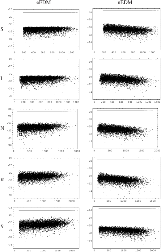
Figure 2: $\mu_{eff}$ versus eEDM (left panels) and nEDM (right panels) in $U(1)^{\prime}$ models (top to bottom: S, I, N, $\psi$ and $\eta$ models). As inputs, all trilinears are scanned in -2 to 2 TeV, all sfermions are scanned in 0.5 to 1 TeV separately. The resulting data sets are used to obtain in every model with $\tan\beta=3$. Absolute value of EDM predictions are given in $\log_{10}$ base, $\mu_{eff}$ values are given in GeVs. Straight lines in this and following figures denote corresponding eEDM and nEDM experimental constraints Regan:2002ta ; Baker:2006ts .

It is also useful to probe how EDM predictions vary with the mass of $Z^{\prime}$ boson, which is given in Fig. 3. The left $\eta$ panel of Fig 3 shows that it may be possible to bound $Z^{\prime}$ mass from above once the eEDM predictions near the present experimental value (at least for certain range of parameters), whereas some models like S and I do not seem to react significantly to this variation. The most sensitive models to bound $Z^{\prime}$ mass using the eEDM results are $\eta$, $\psi$ and N models. On the other hand, it may also be possible to bound the mass of $Z^{\prime}$ in S model using the nEDM measurements, as can be seen from the bottom S panel of Fig. 3.

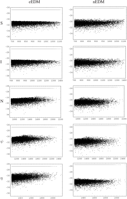
Figure 3: $M_{Z^{\prime}}$ versus eEDM (left panels) and nEDM (right panels) in $U(1)^{\prime}$ models, as in Fig. 2.

Our next figure is Fig. 4 in which electron and neutron EDM predictions are presented for the MSSM and for the aforementioned $U(1)^{\prime}$ models against variations in the phase of bino. In S and I models eEDM predictions are generally well below the MSSM predictions. On the other hand, in $\eta$ model it is possible to get lower predictions for nEDM. Notice that while majority of the points obtained are above the MSSM predictions there are regions where it is possible to obtain smaller EDM values for both of the electron and neutron (i.e. see the gray crosses in N and $\psi$ panels).

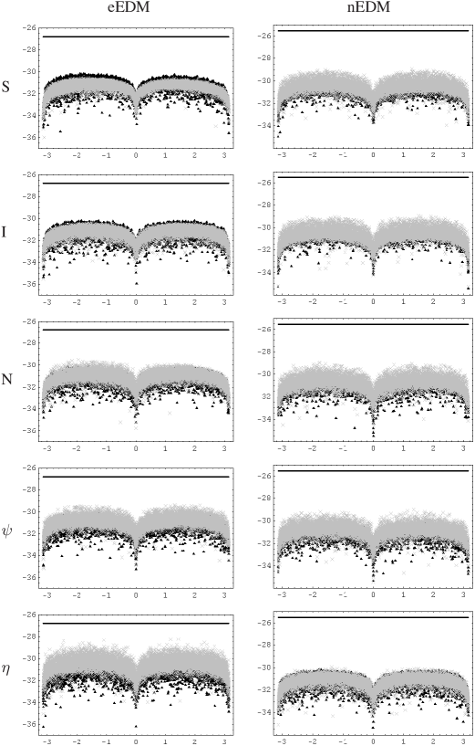
Figure 4: The phase of $M_{1}$ versus eEDM (left panels) and nEDM (right panels) in $U(1)^{\prime}$ models. Here our shading convention is such that dark triangles correspond to MSSM and gray crosses are for $U(1)^{\prime}$ models. Inputs are as in Fig. 2.

As can be deduced from the previous figures there is a hierarchy among the models. This situation is also shared by the mass of the lightest Higgs boson. We provide Fig. 5 in which mass of the lightest Higgs boson is plotted against variations of $\mu_{eff}$. Here again, predictions for the mass of the lightest Higgs boson are in an order increasing from S to $\eta$ model. Notice that while the LEP2 bound on SM like Higgs boson confines its mass to be larger than 114 GeV it can not be used directly in $U(1)^{\prime}$ models, so we accepted 90 GeV as the lower bound. But all of the models are capable of satisfying $m_{h}>114$ GeV. Additionally, compared to the MSSM, in these $U(1)^{\prime}$ models it is possible to find larger $m_{h}$ predictions for $m_{h}$ i.e. see $\eta$ or $\psi$ panels.

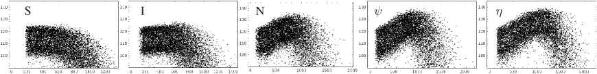
Figure 5: Effective $\mu$ versus $m_{h}$ in $U(1)^{\prime}$ models (All in GeVs). Inputs are the same with Fig. 2.

Another important issue worth noticing within these models is the possibility of kinetic mixing. As should be predicted it modifies EDM predictions (as well as many other properties of the models) in accordance with its magnitude. To give a concrete example of its impact, we selected N model for which eEDM and nEDM predictions are generally larger than the MSSM. So, we provide Fig. 6 for electron and neutron EDMs. As can be seen the very figure, even very small values of the kinetic mixing angle (i.e. $\chi$=-0.1) can yield sizable variations for the EDM predictions of the electron, but, its impact on the neutron EDM is rather small. Meanwhile, nonzero choices of the mass terms $M_{K}$ (see the $c$ panels) can also reduce both of the eEDM and nEDM predictions. When both of the $\chi$ and $M_{K}$ are in charge (see the $d$ panels), we see that, both of the eEDM and nEDM predictions in the N model can be smaller than the MSSM predictions.

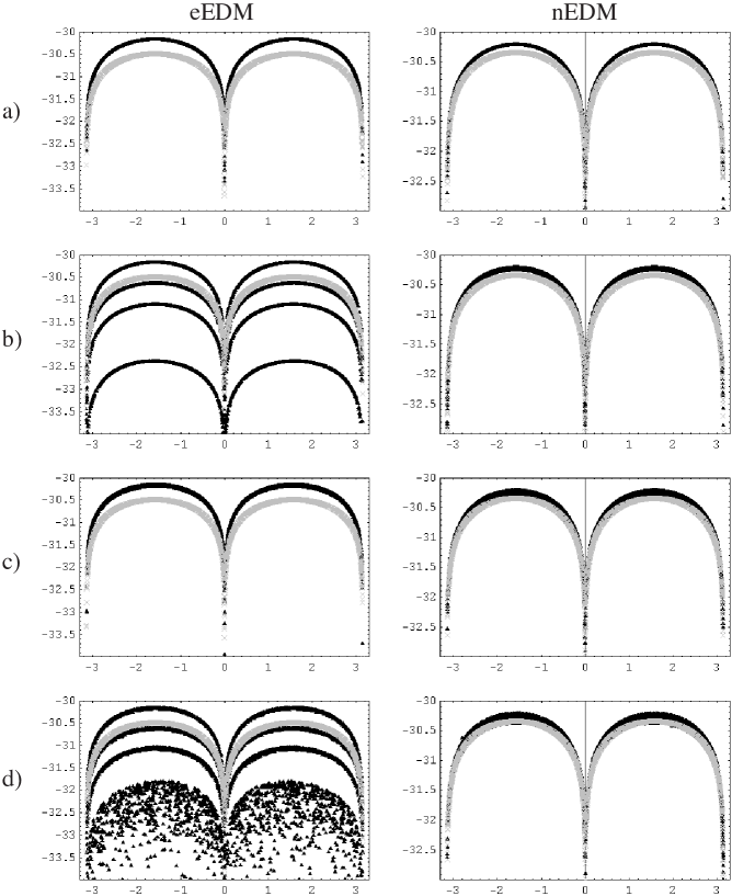
Figure 6: The eEDM (left panels) and the nEDM (right panels) versus argument of $M_{1}$ in N model (Dark triangles : MSSM, gray crosses : N model). Here we fixed $\tan\beta=5$, $m_{\rm{sleptons}}=400$ GeV, $m_{\rm{squarks}}=750$ GeV, all trilinars=-1500 GeV, $M_{2}=190$ GeV ($M_{1}=0.56\,M_{2}$, $M_{3}=2.8\,M_{2}$) In panel a) mixing angle $\chi=0$, $M_{YX}=0$, b) mixing angle $\chi=-0.3,-0.2,-0.1,0$ and $M_{YX}=0$, c) mixing angle $\chi=0$ but $M_{YX}$ scanned randomly in 0 to 0.5 TeV d) $\chi=-0.3,-0.2,-0.1,0$ and $M_{YX}$ scanned randomly in 0 to 0.5 TeV. Notice that $M_{YX}\sim\,M_{K}$ for small $\chi$ values as in our cases (see Choi:2006fz for details)

A rather interesting effect of the kinetic mixing can be investigated on the composition of the LSP candidate of the $U(1)^{\prime}$ models. For the selected range of the parameters, all $U(1)^{\prime}$ models share the same LSP candidate with the MSSM, which is bino. But also notice that singlino dominated neutralino can be a good candidate for the LSP Nakamura:2006ht ; Suematsu:2005bc , for this kind of models.

In our domain, without the kinetic mixing its composition can be expected to be very similar to the MSSM’s lightest neutralino. This can be inferred from Fig. 7 where singlino (gray crosses) and $Z^{\prime}$-ino (dark triangles) compositions of the LSP candidate are plotted against varying $M_{K}$ with (left panel) and without (right panel) the kinetic mixing scanned randomly in [-0.3,0]. Notice that when $M_{K}\sim 0$ GeV, even if the kinetic mixing is turned on, the composition of the LSP candidate can not be expected to be very different from the MSSM.

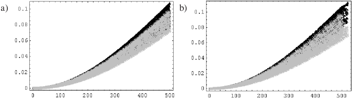
Figure 7: Singlino (gray crosses: $\rm{|N_{1,5}|^{2}}$) and $Z^{\prime}$-ino (dark tringles: $\rm{|N_{1,6}|^{2}}$) compositions of the lightest neutralino against $M_{K}$ in N model. Inputs are from c) and d) panels of Fig. 6. (for a) and b) panels they are of the order $10^{-7}$).

For a clear picture of this phenomena we support Figs. 6 and 7 with Fig. 8, where the mass eigenvalues of the N model neutralinos are plotted against varying $M_{K}$ with (panel b)) and without (panel a)) mixing angle. As can be seen from Fig 8, mass of the LSP candidate of the related model is sensitive to $M_{K}$. This tendency reduces as we go away from the lightest neutralino up to 5th and 6th neutralinos. For those two heavy neutralinos impact of nonzero mixing angle can dominate the effect of $M_{K}$ if both of them are in charge (see panel b) of Fig 8). For the selected range of parameters lightest neutralino is very similar to the MSSM’s neutralino as far as the mentioned variables are off; when they are on, their corresponding impact on the composition and on the mass of the lightest neutralino can be $\sim$ 10-20 $\%$ as can be seen from the very figures.

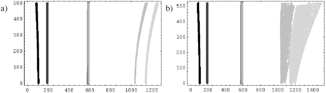
Figure 8: Neutralino masses versus $M_{K}$ corresponding to the same panels of Fig. 7 (All in GeVs).

Our last figure is Fig. 9 where we present $\tan\beta$ dependencies of the electron and neutron EDMs. Here $\tan\beta$ is scanned up to 10 and the most striking difference between the MSSM and $U(1)^{\prime}$ models, for the models under concern, turns out to be the smallness of $\tan\beta$ (can be as small as 0.5), which is ruled out for the MSSM. Additionally, for most of the models eEDM and nEDM predictions decrease with decreasing $\tan\beta$ as in the MSSM. The only exception to this observation is found for $\eta$ model where the sensitivity of eEDM predictions are very small. But, in general, this common tendency of $U(1)^{\prime}$ models show that it is easier to evade EDM constraints in such models where $\tan\beta\sim 1$ is actually the natural value.

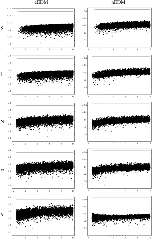
Figure 9: $\tan\beta$ versus eEDM (left panels) and nEDM (right panels) predictions in different $U(1)^{\prime}$ models. We used the conventions of Fig. 3. Here again straight lines denotes the corresponding EDM bounds.

As can be seen from the figures presented in this section, we did not try to constrain complex phases but instead we tried to demonstrate the general tendencies in $U(1)^{\prime}$ models, and apparently all the examples given here are well below the experimental bounds.

IV Conclusion

In this work we have performed a study of EDMs (of electron and neutron) in $U(1)^{\prime}$ models descending from $E(6)$ SUSY GUT. With anticipated increase in precision of EDM measurements, our results show that these models give rise to observable signatures not shared by the MSSM. Indeed, $U(1)^{\prime}$ models generically possess different predictions for EDMs compared to MSSM (see Fig. 4). This very feature provides a way of determining nature of the supersymmetric model at the ${\rm TeV}$ scale via EDM measurements.

Apart from comparisons with the MSSM, different $E(6)$–based $U(1)^{\prime}$ models are found to have different predictions for various observables studied in the text. Indeed, sensitivity of EDMs to $\mu$ parameter (see Fig. 2), to $Z^{\prime}$ mass (see Fig. 3), and to $\tan\beta$ are different for different models. Furthermore, eEDM and nEDM are found to exhibit different dependencies in each case. These features establish the fact that, once precise measurements are attained (presumably at a high-energy linear collider) one can determine likely breaking directions for $E(6)$ grand unified group down to that of the MSSM.

Fig. 6 makes it clear that the soft-breaking mass that mix $U(1)_{Y}$ and $U(1)^{\prime}$ gauginos is a sensitive source of EDMs. Indeed, as happens in models of paraphotons, entire matter can be neutral under $U(1)^{\prime}$ symmetry yet such a kinetic mixing (that mix gauge bosons and gauginos ) can exist and can have important implications. These figures make it clear that EDMs vary significantly with this parameter.

Also interesting are the predictions of different $U(1)^{\prime}$ models for $m_{h}$ (which is plotted against $\mu_{eff}$ in Fig. 5). Indeed, both range and shape of the allowed domain are different for different models, and this feature also helps determining the correct model (of $E(6)$ origin) once precise measurements of associated quantities are available.

It is not surprising that these models can have important implications also for FCNC observables (including their CP asymmetries) langackerx . Moreover, the EDMs discussed above can be correlated with the CP asymmetries (of $B$ meson decays correlate ) or with the Higgs sector itself correlate2 so as to further bound such models with the information available from $B$ factories and Tevatron. This kind of analysis will be given elsewhere.

To conclude, the problem of CP violation (in particular EDMs) is a particularly important issue of $U(1)^{\prime}$ models for various reasons, most notably, the approximate reality of the effective $\mu$ parameter. Analyses of various observables (including the FCNC ones) can shed further light on the origin and structure of such models.

V Acknowledgments

We all would like to thank to D. A. DEMİR for his contributions with inspiring and illuminating discussions in various stages of this work.

References

- (1) J. E. Kim and H. P. Nilles, Phys. Lett. B 138, 150 (1984); D. Suematsu and Y. Yamagishi, Int. J. Mod. Phys. A 10, 4521 (1995) [arXiv:hep-ph/9411239]; M. Cvetic and P. Langacker, Mod. Phys. Lett. A 11, 1247 (1996) [arXiv:hep-ph/9602424]; V. Jain and R. Shrock, arXiv:hep-ph/9507238; Y. Nir, Phys. Lett. B 354, 107 (1995) [arXiv:hep-ph/9504312].
- (2) R. W. Robinett and J. L. Rosner, Phys. Rev. D 25, 3036 (1982) [Erratum-ibid. D 27, 679 (1983)].
- (3) R. W. Robinett and J. L. Rosner, Phys. Rev. D 26, 2396 (1982).
- (4) P. Langacker, R. W. Robinett and J. L. Rosner, Phys. Rev. D 30, 1470 (1984).
- (5) M. Cvetic and P. Langacker, Phys. Rev. D 54, 3570 (1996) [arXiv:hep-ph/9511378].
- (6) M. Cvetic and P. Langacker, Mod. Phys. Lett. A 11, 1247 (1996) [arXiv:hep-ph/9602424].
- (7) D. A. Demir, L. Solmaz and S. Solmaz, Phys. Rev. D 73, 016001 (2006) [arXiv:hep-ph/0512134].
- (8) D. Suematsu, Phys. Rev. D 59 (1999) 055017 [arXiv:hep-ph/9808409].
- (9) S. F. King, S. Moretti and R. Nevzorov, Phys. Rev. D 73 (2006) 035009 [arXiv:hep-ph/0510419].
- (10) D. A. Demir, G. L. Kane and T. T. Wang, Phys. Rev. D 72 (2005) 015012 [arXiv:hep-ph/0503290].
- (11) P. Langacker, arXiv:0801.1345 [hep-ph].
- (12) S. Y. Choi, H. E. Haber, J. Kalinowski and P. M. Zerwas, Nucl. Phys. B 778 (2007) 85 [arXiv:hep-ph/0612218].
- (13) D. A. Demir, L. L. Everett and P. Langacker, Phys. Rev. Lett. 100, 091804 (2008) [arXiv:0712.1341 [hep-ph]].
- (14) J. A. Aguilar-Saavedra et al., Eur. Phys. J. C 46, 43 (2006) [arXiv:hep-ph/0511344].
- (15) D. A. Demir and L. L. Everett, Phys. Rev. D 69, 015008 (2004) [arXiv:hep-ph/0306240].
- (16) M. Cvetic, D. A. Demir, J. R. Espinosa, L. L. Everett and P. Langacker, Phys. Rev. D 56, 2861 (1997) [Erratum-ibid. D 58, 119905 (1998)] [hep-ph/9703317].
- (17) J. Dai, H. Dykstra, R. G. Leigh, S. Paban and D. Dicus, Phys. Lett. B 237 (1990) 216 [Erratum-ibid. B 242 (1990) 547].
- (18) S. Abel, S. Khalil and O. Lebedev, Nucl. Phys. B 606 (2001) 151 [arXiv:hep-ph/0103320].
- (19) T. Ibrahim and P. Nath, Phys. Rev. D 57 (1998) 478 [Erratum-ibid. D 58 (1998 ERRAT,D60,079903.1999 ERRAT,D60,119901.1999) 019901] [arXiv:hep-ph/9708456].
- (20) M. Masip and A. Pomarol, Phys. Rev. D 60, 096005 (1999) [arXiv:hep-ph/9902467].
- (21) D. Suematsu, Mod. Phys. Lett. A 12 (1997) 1709 [arXiv:hep-ph/9705412].
- (22) S. Nakamura and D. Suematsu, Phys. Rev. D 75, 055004 (2007) [arXiv:hep-ph/0609061].
- (23) D. Suematsu, Phys. Rev. D 73, 035010 (2006) [arXiv:hep-ph/0511299].
- (24) P. Langacker and M. Plumacher, Phys. Rev. D 62, 013006 (2000) [arXiv:hep-ph/0001204].
- (25) T. M. Aliev, D. A. Demir, E. Iltan and N. K. Pak, Phys. Rev. D 54, 851 (1996) [arXiv:hep-ph/9511352].
- (26) D. A. Demir, Phys. Lett. B 571, 193 (2003) [arXiv:hep-ph/0303249]; A. Dedes and A. Pilaftsis, Phys. Rev. D 67, 015012 (2003) [arXiv:hep-ph/0209306]; M. S. Carena, A. Menon, R. Noriega-Papaqui, A. Szynkman and C. E. M. Wagner, Phys. Rev. D 74, 015009 (2006) [arXiv:hep-ph/0603106].
- (27) B. C. Regan, E. D. Commins, C. J. Schmidt and D. DeMille, Phys. Rev. Lett. 88 (2002) 071805.
- (28) C. A. Baker et al., Phys. Rev. Lett. 97, 131801 (2006) [arXiv:hep-ex/0602020].