Using a squeezed field to protect two-atom entanglement against spontaneous emissions

Abstract

Tunable interaction between two atoms in a cavity is realized by interacting the two atoms with an extra controllable single-mode squeezed field. Such a controllable interaction can be further used to control entanglement between the two atoms against amplitude damping decoherence caused by spontaneous emissions. For the independent amplitude damping decoherence channel, entanglement will be lost completely without controls, while it can be partially preserved by the proposed strategy. For the collective amplitude damping decoherence channel, our strategy can enhance the entanglement compared with the uncontrolled case when the entanglement of the uncontrolled stationary state is not too large.

1 Introduction

Quantum entanglement [1, 2, 3, 4, 5, 6] is a fundamental property of multi-body quantum systems that shows the non-local feature of quantum states. Quantum entanglement has been commonly recognized to be an essential physical resource in the implementation of high-speed quantum computation and high-security quantum communication.

Many efforts have been made to create entanglement between decoupled quantum systems. One natural way is to introduce a simple intermediate device [7, 8, 9, 10, 11], e.g., a single-mode field or an additional particle, whose coherent interactions with the systems lead to their indirect interactions with each other. The intermediate device can also be measured to extract information about the quantum systems for quantum feedback controls [12, 13, 14] to manipulate the entanglement dynamics. One may also utilize a dissipative environment [15, 16, 17, 18], e.g., a collective decoherence environment, to generate entanglement, interacted with which the system irreversibly decays to a stationary entangled state.

However, in most circumstances, quantum entanglement tends to be destructed in environments [19, 20, 21, 22]. For example, independent decoherence channels always lead to disentanglement [23] that is not recoverable by local operations and classical communications.

Generally, non-local operations are required to effectively protect entanglement. However, a non-local Hamiltonian generated from the internal interaction between quantum systems, e.g., the dipole-dipole interaction between two atoms via the vacuum, is sometimes not a good choice, because disentanglement can also be induced by decoherence under these interactions.

This paper introduces a single-mode squeezed field in a quantum cavity to realize non-local controllable interactions between two identical atoms in the weak coupling regime. By altering the parameter amplification coefficient of the squeezed field, one can continuously adjust the coupling strengths between atoms, which can be further used to control the final entanglement between the two atoms in presence of decoherence. It should be pointed out that there is another interesting work on coupling the two atoms via the squeezed vacuum [24]. Compared with the squeezed vacuum, the auxiliary squeezed field in the cavity is more controllable, which would be helpful to control the stationary concurrence.

The paper is organized as follows: the physical model applied in the paper is formulated in Sec. 2. Entanglement control strategies are discussed for two-atom independent amplitude damping decoherence channels, collective amplitude damping decoherence channels, and their mixture, respectively in Sec. 3, 4 and 5. Conclusions and a forecast of the future work are drawn in Sec. 6.

2 Model Formulation

Consider the system of two identical two-level atoms interacting with a squeezed single-mode field in a quantum cavity (see Fig. 1).

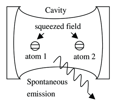
Figure 1: Two atoms undergoing decoherence caused by spontaneous emissions interact with a single-mode squeezed field in a cavity.

The total Hamiltonian of the atoms and the cavity mode can be described as below with $\hbar$ assumed to be $1$ without loss of generality:

$$H_{AC} = \omega_{c}a^{\dagger}a+\frac{\omega_{a}}{2}\sum_{i=1}^{2}\sigma_{z}^{(i)}+\sum_{i=1}^{2}(\epsilon^{(i)}a\sigma_{+}^{(i)}+\epsilon^{(i)*}a^{\dagger}\sigma_{-}^{(i)})$$ (1)

$$+(\xi e^{-i\Omega t}a^{\dagger\,2}+\xi^{*}e^{i\Omega t}a^{2}),$$

where the first two terms describe the free Hamiltonians of the cavity mode and the atoms; $\omega_{c}$ is the frequency of the cavity mode and $\omega_{a}$ is the inherent frequency of the atom corresponding to the energy separation between the ground state and the excited state of each atom; $a$ is the annihilation operator of the cavity mode and $\sigma_{z}^{(i)},\,i=1,2$ is the $z$-axis Pauli operator of the $i$-th atom. The third term represents the interaction between the atoms and the cavity mode, in which $\sigma_{\pm}^{(i)}=\sigma_{x}^{(i)}\pm i\sigma_{y}^{(i)},\,i=1,2$, are the ladder operators of the $i$-th atom. The complex coefficient

$$\epsilon^{(i)}=\vec{\mu}\cdot\vec{g}(\vec{r}^{(i)}),$$

is the inner product of the transition dipole moment $\vec{\mu}$ of each atom and the coupling constant

$$\vec{g}(\vec{r}^{(i)})=\left(\frac{\omega_{c}}{2\epsilon_{0}V}\right)^{\frac{1}{2}}\hat{e}_{\vec{k}}e^{i\vec{k}\cdot\vec{r}^{(i)}},$$ (2)

where $\vec{r}^{(i)}$ is the position of the $i$-th atom; $\vec{k}$ and $\hat{e}_{\vec{k}}$ are the wave vector and unit polarization vector of the cavity mode; and $V$ is the normalization volume of the cavity mode. The last term is the Hamiltonian of the squeezed cavity mode, where the parameter amplification coefficient $\xi$ and the frequency $\Omega$ are continuously tunable. Such a manipulable standing squeezed field in a high-Q cavity is realizable by squeezed state engineering developed recently [26, 27]. Roughly speaking, a three-level atom in a ladder configuration is introduced to interact with the cavity mode. In addition, a classical field is used to manipulate the three-level atom, through which one can continuously adjust the squeezed coefficient $\xi$ and the frequency $\Omega$.

In the weak coupling regime, i.e., $\Delta=\omega_{a}-\omega_{c}$ and $|\xi|\gg|\epsilon^{(i)}|$, $H_{AC}$ can be diagonalized by the following unitary transform [28]:

$$U=\exp\left[\frac{1}{\Delta}\sum_{i=1}^{2}(\epsilon^{(i)}a\sigma_{+}^{(i)}-\epsilon^{(i)*}a^{\dagger}\sigma_{-}^{(i)})\right],$$

which, by taking the first-order approximation of $\epsilon^{(i)}/\Delta$, gives the following expression:

$$H_{AC}\approx UH_{AC}U^{\dagger} \approx \omega_{c}a^{\dagger}a+\xi e^{-i\Omega t}a^{\dagger\,2}+\xi^{*}e^{i\Omega t}a^{2}$$

$$+\sum_{i=1}^{2}\left[\frac{\tilde{\omega}_{a}}{2}+\frac{4|\epsilon^{(i)}|^{2}}{\Delta^{2}}\left(\xi e^{-i\Omega t}a^{\dagger\,2}+{\rm h.c.}\right)+\frac{4|\epsilon^{(i)}|^{2}}{\Delta}a^{\dagger}a\right]\sigma^{(i)}_{z}$$

$$+\sum_{i=1}^{2}\left[\left(\frac{2\epsilon^{(i)}\xi e^{-i\Omega t}}{\Delta}a^{\dagger}+\frac{|\epsilon^{(i)}|^{2}\xi e^{-i\Omega t}}{\Delta^{2}}\right)\sigma_{+}^{(i)}+{\rm h.c.}\right]$$

$$+\left(\mu_{1}e^{-i(\Omega t+\phi_{1})}\sigma_{+}^{(1)}\sigma_{+}^{(2)}+{\rm h.c.}\right)$$

$$+\left(\mu_{2}e^{-i\phi_{2}}\sigma_{+}^{(1)}\sigma_{-}^{(2)}+{\rm h.c.}\right),$$

where ${\rm h.c.}$ refers to Hermitian conjugate;

$$\tilde{\omega}_{a}=\omega_{a}+\frac{2\left(|\epsilon^{(1)}|^{2}+|\epsilon^{(2)}|^{2}\right)}{\Delta},\,\,\,\mu_{1}e^{-i\phi_{1}}=\frac{2\xi\epsilon^{(1)}\epsilon^{(2)}}{\Delta^{2}},\,\,\,\mu_{2}e^{-i\phi_{2}}=\frac{\epsilon^{(1)}\epsilon^{(2)*}}{\Delta}.$$

Further, by adiabatically eliminating the degrees of freedom of the cavity mode, the following reduced two-atom Hamiltonian can be obtained:

$$H_{A}=\frac{\omega_{a}}{2}\sum_{i=1}^{2}\sigma_{z}^{(i)}+\left(\mu_{1}e^{-i(\Omega t+\phi_{1})}\sigma_{+}^{(1)}\sigma_{+}^{(2)}+{\rm h.c.}\right)+\left(\mu_{2}e^{-i\phi_{2}}\sigma_{+}^{(1)}\sigma_{-}^{(2)}+{\rm h.c.}\right),$$

where the terms of individual atomic interaction with the cavity are omitted due to the fact that

$$\frac{\omega_{a}}{2}{\gg}|\epsilon^{(i)}|^{2}/\Delta,\,|\xi\epsilon^{(i)}|/\Delta$$

under the large detuning condition $\Delta\gg\epsilon^{(i)}$. Since the parameter amplification coefficient $\xi$ and the frequency $\Omega$ are tunable parameters, we have two control parameters $\mu_{1}$ and $\Omega$ in $H_{A}$. In the interaction picture, $H_{A}$ can be expressed as:

$$H_{A}^{\rm eff} = \left(\mu_{1}e^{-i\phi_{1}}\sigma_{+}^{(1)}\sigma_{+}^{(2)}+\mu_{1}e^{i\phi_{1}}\sigma_{-}^{(1)}\sigma_{-}^{(2)}\right)+\left(\mu_{2}e^{-i\phi_{2}}\sigma_{+}^{(1)}\sigma_{-}^{(2)}+\mu_{2}e^{i\phi_{2}}\sigma_{-}^{(1)}\sigma_{+}^{(2)}\right),$$ (3)

when the parameter $\Omega$ is fixed to be $2\omega_{a}$.

Besides the cavity mode, the atoms also interact with other modes in the environment, which leads to the atomic spontaneous emissions. In the case that the environmental modes are at the vacuum state, the dynamics of atoms can be described by the following master equation [18, 25]:

$$\dot{\rho}=-i[H_{A}^{\rm eff}+H_{12},\rho]+\sum_{i,j=1}^{2}\Gamma_{ij}\left(\sigma_{-}^{(i)}\rho\sigma_{+}^{(j)}-\frac{1}{2}\rho\sigma_{+}^{(j)}\sigma_{-}^{(i)}-\frac{1}{2}\sigma_{+}^{(j)}\sigma_{-}^{(i)}\rho\right).$$ (4)

The parameters

$$\Gamma_{11}=\Gamma_{22}=\Gamma=\frac{\omega_{a}^{3}\mu^{2}}{3\pi\epsilon_{0}c^{3}}$$ (5)

are the spontaneous emission rates of the individual atoms, where $\mu=|\vec{\mu}|$ is the magnitude of the transition dipole momentum, while

$$\Gamma_{12}=\Gamma_{21}=\Gamma F(k_{0}r_{12})$$ (6)

represent the collective spontaneous emission rates induced by the coupling between the atoms. The function $F(k_{0}r_{12})$ can be expressed as [18, 25]:

$$F(k_{0}r_{12})=\frac{3}{2}\left\{(1-3\cos^{2}\theta)\left[\frac{\cos(k_{0}r_{12})}{(k_{0}r_{12})^{2}}-\frac{\sin(k_{0}r_{12})}{(k_{0}r_{12})^{3}}\right]+\sin^{2}\theta\frac{\sin(k_{0}r_{12})}{k_{0}r_{12}}\right\},$$

where $k_{0}=\omega_{a}/c$ and $\theta$ is the angle between the dipole moment vector $\vec{\mu}$ and the vector $\vec{r}_{12}=\vec{r}^{(1)}-\vec{r}^{(2)}$; $r_{12}=|\vec{r}_{12}|$ is the distance between the two atoms. The spontaneous emission process also introduces an additional coherent dipole-dipole interaction between the atoms:

$$H_{12}=\eta(\sigma_{+}^{(1)}\sigma_{-}^{(2)}+\sigma_{-}^{(1)}\sigma_{+}^{(2)}),$$

where the coefficient $\eta$ in $H_{12}$ can be written as [25]:

$$\eta = \frac{3}{4}\Gamma\left\{[1-3\cos^{2}\theta]\left[\frac{\sin(k_{0}r_{12})}{(k_{0}r_{12})^{2}}+\frac{\cos(k_{0}r_{12})}{(k_{0}r_{12})^{3}}\right]-\sin^{2}\theta\frac{\cos(k_{0}r_{12})}{k_{0}r_{12}}\right\}.$$ (7)

3 Independent amplitude damping decoherence channel

When the distance $r_{12}$ between the two atoms is far greater than the resonant wavelength $1/k_{0}=c/\omega_{a}$ of the atom, i.e., $k_{0}r_{12}\rightarrow\infty$, the amplitude damping decoherence of the two atoms can be taken independently. Consequently, from Eqs. (6) and (7), we have $\eta,\,\Gamma_{12},\,\Gamma_{21}\rightarrow 0$, from which the following master equation holds:

$$\dot{\rho}=-i[H_{A}^{\rm eff},\rho]+\Gamma\mathbb{D}[\sigma_{-}^{(1)}]\rho+\Gamma\mathbb{D}[\sigma_{-}^{(2)}]\rho,$$ (8)

where the superoperator $\mathbb{D}[L]\rho$ is defined as:

$$\mathbb{D}[L]\rho=L\rho L^{\dagger}-\frac{1}{2}L^{\dagger}L\rho-\frac{1}{2}\rho L^{\dagger}L,$$

and the two Lindblad terms $\mathbb{D}[\sigma_{-}^{(1)}]\rho$, $\mathbb{D}[\sigma_{-}^{(2)}]\rho$ represent the amplitude damping decoherence channels acting on the two atoms with the damping rate $\Gamma>0$.

To measure the quantum entanglement, we use the concurrence [3] between the two atoms of the quantum state $\rho$:

$$C(\rho)=\max\{\lambda_{1}-\lambda_{2}-\lambda_{3}-\lambda_{4},0\},$$ (9)

where $\lambda_{i}^{\prime}s$ are the square roots of the eigenvalues, in decreasing order, of the matrix:

$$M=\rho(\sigma_{y}^{(1)}\sigma_{y}^{(2)})\rho^{*}(\sigma_{y}^{(1)}\sigma_{y}^{(2)}),$$

and $\rho^{*}$ is the complex conjugate of $\rho$.

It is known that, in absence of the squeezed field, a two-atom system will always be disentangled under independent amplitude damping decoherence channels (see, e.g., Ref. [23]), and this is not recoverable by any local operations. However, the entanglement can be partially protected via the intermediate squeezed field, because the solution $\rho(t)$ of Eq. (8) tends to a stationary state

$$\rho_{\infty}=\frac{2\mu_{1}\Gamma}{4\mu_{1}^{2}+\Gamma^{2}}\rho_{m}+\left(1-\frac{2\mu_{1}\Gamma}{4\mu_{1}^{2}+\Gamma^{2}}\right)\rho_{s},$$ (10)

as a convex combination of a pure maximally entangled state

$$\rho_{m}(\phi_{1})=\frac{1}{2}\left(\begin{array}[]{cccc}1&&&e^{-i\left(\phi_{1}-\frac{\pi}{2}\right)}\\ &0&&\\ &&0&\\ e^{i\left(\phi_{1}-\frac{\pi}{2}\right)}&&&1\\ \end{array}\right)$$ (11)

and a diagonal separable state

$$\rho_{s}={\rm diag}(1-3\beta,\,\beta,\,\beta,\,\beta),$$

where

$$\beta=\frac{1}{8}\left(1-\sqrt{1-\left(\frac{4\mu_{1}\Gamma}{4\mu_{1}^{2}+\Gamma^{2}}\right)^{2}}\right).$$

The subscript “$m$” is an abbreviation of “maximally entangled”, and the subscript “$s$” refers to “separable”. The corresponding stationary concurrence is:

$$C(\rho_{\infty})=\max\left\{\frac{2\mu_{1}(\Gamma-\mu_{1})}{4\mu_{1}^{2}+\Gamma^{2}},0\right\},$$ (12)

which, when the coupling strength $\mu_{1}$ is tuned to be

$$\mu_{1}=\frac{1}{\sqrt{5}+1}\Gamma,$$

reaches its maximum value:

$$C_{\rm max}=\frac{\sqrt{5}-1}{4}\approx 0.31>0.$$

The plot of $C(\rho_{\infty})$ versus $\mu_{1}/\Gamma$ is shown in Fig. 2.

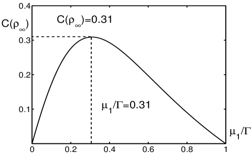
Figure 2: Plot of $C(\rho_{\infty})$ versus $\mu_{1}/\Gamma$.

The cumbersome proof of Eqs. (10) and (12) is shown in A. We adopt here an ideal model in which the two atoms have precise positions $\vec{r}^{(i)}$. In real systems, position fluctuations are always presented, i.e.,

$$\tilde{\vec{r}}^{(i)}=\vec{r}^{(i)}+\delta\vec{r}^{(i)},\,\,\,i=1,2,$$

where $\tilde{\vec{r}}^{(i)}$ is the actual position of the $i$-th atom and $\delta\vec{r}^{(i)}$ is the corresponding fluctuation. From Eq. (2), the actual coupling coefficients should be

$$\tilde{\mu}_{1}e^{i\tilde{\phi}_{1}}=e^{i\vec{k}\cdot(\delta\vec{r}^{(1)}+\delta\vec{r}^{(2)})}\mu_{1}e^{i\phi_{1}}=\mu_{1}e^{i(\phi_{1}+\vec{k}\cdot(\delta\vec{r}^{(1)}+\delta\vec{r}^{(2)}))},$$

which, consequently, fluctuates the phase by

$$\delta\phi_{1}=\tilde{\phi}_{1}-\phi_{1}=\vec{k}\cdot(\delta\vec{r}^{(1)}+\delta\vec{r}^{(2)})=\delta\phi^{(1)}+\delta\phi^{(2)}$$ (13)

for the pure maximally entangled state $\rho_{m}$ (which now it should be $\rho_{m}(\tilde{\phi}_{1})=\rho_{m}(\phi_{1}+\delta\phi_{1})$) due to the fluctuations of the positions of the atoms. Assume that $\delta\phi^{(1)}$ and $\delta\phi^{(2)}$ obey Gaussian distributions with means $0$ and variances $2\gamma_{1}$ and $2\gamma_{2}$, one can verify by averaging over the random fluctuations that the pure maximally entangled state $\rho_{m}$ is blurred into a mixed state:

$$\bar{\rho}_{m} = \int_{-\infty}^{+\infty}\frac{d\delta\phi^{(1)}}{\sqrt{4\pi\gamma_{1}}}e^{-(\delta\phi^{(1)})^{2}/4\gamma_{1}}\int_{-\infty}^{+\infty}\frac{d\delta\phi^{(2)}}{\sqrt{4\pi\gamma_{2}}}e^{-(\delta\phi^{(2)})^{2}/4\gamma_{2}}\rho_{m}(\tilde{\phi}_{1})$$

$$= \frac{1}{2}\left(\begin{array}[]{cccc}1&&&e^{-(\gamma_{1}+\gamma_{2})}e^{-i\left(\phi_{1}-\frac{\pi}{2}\right)}\\ &0&&\\ &&0&\\ e^{-(\gamma_{1}+\gamma_{2})}e^{i\left(\phi_{1}-\frac{\pi}{2}\right)}&&&1\\ \end{array}\right).$$

Apparently, the resulting entanglement is also reduced. In fact, in this case, the stationary state should be

$$\bar{\rho}_{\infty}=\frac{2\mu_{1}\Gamma}{4\mu_{1}^{2}+\Gamma^{2}}\bar{\rho}_{m}+\left(1-\frac{2\mu_{1}\Gamma}{4\mu_{1}^{2}+\Gamma^{2}}\right)\rho_{s},$$

with a modified stationary concurrence

$$C(\bar{\rho}_{\infty})=\left\{e^{-(\gamma_{1}+\gamma_{2})}\frac{2\mu_{1}\Gamma}{4\mu_{1}^{2}+\Gamma^{2}}-\frac{2\mu_{1}^{2}}{4\mu_{1}^{2}+\Gamma^{2}},\,0\right\}.$$

The corresponding maximum stationary concurrence can be further calculated as:

$$\bar{C}_{\rm max}=\frac{1}{4}\left(\sqrt{4e^{-(\gamma_{1}+\gamma_{2})}+1}-1\right).$$

Obviously, we have $\bar{C}_{\rm max}>0$, which means that our strategy is still valid compared with the case without the squeezed field.

However, the maximum stationary concurrence is reduced by the dephasing effects caused by the fluctuations of the positions of the atoms. In order to estimate the influence of the fluctuations on the stationary entanglement, it can be estimated from Eq. (13) that:

$$\gamma_{i}=\frac{1}{2}{\rm var}(\delta\phi^{(i)})\leq\frac{1}{2}|\vec{k}|^{2}{\rm var}\left(|\delta\vec{r}^{(i)}|\right)=2\pi^{2}\left(\frac{\delta r^{(i)}}{\lambda}\right)^{2},$$

where $\lambda$ is the wavelength of the field in the cavity; ${\rm var}(\delta\phi^{(i)})$ is the variance of $\delta\phi^{(i)}$ and $\delta{r}^{(i)}=\sqrt{{\rm var}(|\delta\vec{r}^{(i)}|)}$ represents the magnitude of the position fluctuation for the $i$-th atom. Therefore, if one is capable of trapping the atom in the cavity such that

$$\delta{r}^{(i)}\ll\lambda,$$ (15)

the dephasing coefficients $\gamma_{i}$ can be neglected. This is possible under the present atom trapping and cooling technique since the wavelength $\lambda$ is of the order of $\mu$m (see, e.g., Refs. [29, 30, 31, 32]). In this case, the perturbed maximum stationary concurrence $\bar{C}_{\rm max}$ is deviated slightly from the ideal maximum stationary concurrence $C_{\rm max}$ (e.g., $\bar{C}_{\rm max}/C_{\rm max}\approx 90\%$ when $\delta{r}^{(i)}/\lambda=0.05$ as assumed in Ref. [29]). We can also see the influence from the following example with parameters given in Ref. [30], in which the mass $m$ of the atom (Cs atom), the oscillating frequency $\omega$ of the external freedom of the atom (which is different from $\omega_{a}$), the effective temperature $T_{\rm eff}$ of the atom, and the wavelength $\lambda$ of the field in the cavity are given as:

$$m=133\times 1.66\times 10^{-27}{\rm kg}\approx 2.2\times 10^{-25}{\rm kg},$$

$$\omega=2\pi\times 0.53\times 10^{6}{\rm Hz}\approx 3.3\times 10^{6}{\rm Hz},$$

$$T_{\rm eff}=1.3\times 10^{-4}{\rm K},\,\,\,\lambda\approx 0.9\times 10^{-6}{\rm m}.$$

Here, we choose an effective temperature $T_{\rm eff}$ of the atom that is ten times greater than the lowest cooling temperature ($13\mu{\rm K}$) given in Ref. [30], under which the position of the atom can be taken as a classical parameter because

$$\hbar\omega\ll\frac{1}{2}k_{B}T_{\rm eff},$$

where $k_{B}$ is the Boltzmann constant. In this case, the position fluctuation of the atom can be estimated from

$$\frac{1}{2}m\omega^{2}(\delta{r}^{(i)})^{2}=\frac{1}{2}k_{B}T_{\rm eff},$$

which leads to

$$\delta{r}^{(i)}=\sqrt{\frac{k_{B}T_{\rm eff}}{m\omega^{2}}}=\sqrt{\frac{1.38\times 10^{-23}\times 1.3\times 10^{-4}}{2.2\times 10^{-25}\times 3.3^{2}\times 10^{12}}}\approx 2.7\times 10^{-8}{\rm m}.$$

Thus, we have

$$\frac{\delta{r}^{(i)}}{\lambda}\approx\frac{2.8\times 10^{-8}}{0.9\times 10^{-6}}=0.03,$$

from which it can be calculated that $\bar{C}_{\rm max}/C_{\rm max}\approx 97\%$.

Although the stationary concurrence may not be strong enough to be directly applied in quantum information processing and would be deteriorated by dephasing effects caused by noises such as the position fluctuations of the atoms, it is still hopeful to be used for entanglement protection. In fact, the fidelity between the stationary state $\bar{\rho}_{\infty}$ and the maximally entangled state $\rho_{m}$ can be calculated as:

$$F(\bar{\rho}_{\infty})={\rm tr}(\bar{\rho}_{\infty}\rho_{m})=\frac{e^{-(\gamma_{1}+\gamma_{2})}\mu_{1}\Gamma-\mu_{1}^{2}}{4\mu_{1}^{2}+\Gamma^{2}}+\frac{1}{2}.$$

Optimally, it should be

$$\bar{F}_{\rm max}=\frac{1}{8}\left(\sqrt{4e^{-(\gamma_{1}+\gamma_{2})}+1}-1\right)+\frac{1}{2}>\frac{1}{2}.$$ (16)

Since the maximum fidelity $\bar{F}_{\rm max}$ is always larger than $0.5$, we can, in principle, increase the stationary entanglement by introducing additional entanglement purification process [33, 34].

To illustrate our proposal, let us discuss their applications in some typical circumstances. Firstly, consider the initial states $\rho_{0}^{1}$ at the maximally entangled state

$$\rho_{0}^{1}=\frac{1}{2}\left(\begin{array}[]{cccc}1&&&1\\ &0&&\\ &&0&\\ 1&&&1\\ \end{array}\right),$$

and $\rho_{0}^{2}$ at the mixed entangled state

$$\rho_{0}^{2}=\left(\begin{array}[]{cccc}0.85&&&0.1\\ &0.03&&\\ &&0.07&\\ 0.1&&&0.05\\ \end{array}\right).$$

Moreover, let $\Gamma=1/\tau_{0}$, where $\tau_{0}$ is the relaxing time constant. Simulation results are shown in Fig. 3.

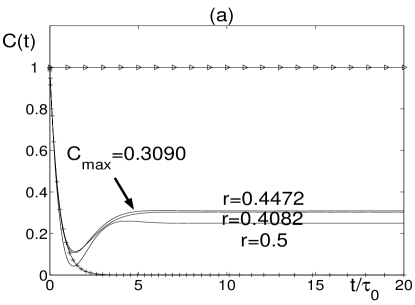
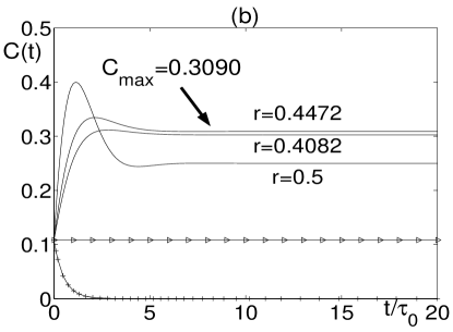
Figure 3: Plots of concurrence $C(t)$ where the initial states are chosen as (a) maximally entangled state $\rho_{0}^{1}$ and (b) mixed entangled state $\rho_{0}^{2}$. The plus-sign lines denote the uncontrolled trajectories; the triangle lines are for the free trajectories in absence of control and decoherence; the solid lines represent the controlled trajectories with chosen parameters $r=2\mu_{1}\Gamma/(4\mu_{1}^{2}+\Gamma^{2})$, which is the proportion of the maximally entangled state $\rho_{m}$ in Eq. (10).

It is shown in Fig. 3 that the entanglement of the quantum states always decays to zero without control as what is known in the literature [23]. The corresponding stationary state is the two-atom ground state:

$$\rho^{u}_{\infty}=|00\rangle\langle 00|=\left(\begin{array}[]{cccc}1&&&\\ &0&&\\ &&0&\\ &&&0\\ \end{array}\right),$$

which is at the boundary of the set of all separable states. The superscript “$u$” refers to the “uncontrolled” system. When our strategy is applied, the entanglement can be remarkably retrieved against decoherence, and the maximum concurrence of the stationary state is

$$C_{\max}=\frac{\sqrt{5}-1}{4}\approx 0.31,$$

when

$$r=\frac{2\mu_{1}\Gamma}{4\mu_{1}^{2}+\Gamma^{2}}=\frac{1}{\sqrt{5}}\approx 0.45.$$

It is also noted that our strategy can enhance the entanglement of the stationary state of the naked atoms (i.e., neither control nor decoherence exist).

4 Collective amplitude damping decoherence channel

When the distance between the atoms is far shorter than the resonant wavelength of the atom, i.e., $k_{0}r_{12}\rightarrow 0$, from Eqs. (6) and (7) we have:

$$\eta\rightarrow\eta_{0}=\frac{3\Gamma}{4k_{0}^{3}r_{12}^{3}}(1-3\cos^{2}\theta),\,\,\,\Gamma_{12}=\Gamma_{21}\rightarrow\Gamma,$$

which corresponds to a two-atom collective amplitude damping decoherence channel [35]. In this case, the master equation of the two atoms becomes:

$$\dot{\rho} = -i\left[H_{A}^{\rm eff}+\eta_{0}\left(\sigma_{+}^{(1)}\sigma_{-}^{(2)}+\sigma_{-}^{(1)}\sigma_{+}^{(2)}\right),\rho\right]+\Gamma\mathbb{D}[S_{-}]\rho,$$ (17)

where the two-atom operator $S_{-}=\sigma_{-}^{(1)}+\sigma_{-}^{(2)}$, and $\Gamma>0$ is the damping rate. Because the two atoms are very close to each other, from Eq. (2) the coupling strength between each atom and the cavity can be taken as identical, i.e., $\epsilon^{(1)}=\epsilon^{(2)}=\epsilon$, so that the interaction Hamiltonian $H_{A}^{\rm eff}$ can be expressed as:

$$H_{A}^{\rm eff}=\mu_{1}\left(e^{-i\phi_{1}}\sigma_{+}^{(1)}\sigma_{+}^{(2)}+e^{i\phi_{1}}\sigma_{-}^{(1)}\sigma_{-}^{(2)}\right)+\mu_{2}\left(\sigma_{+}^{(1)}\sigma_{-}^{(2)}+\sigma_{-}^{(1)}\sigma_{+}^{(2)}\right),$$

where

$$\mu_{1}e^{-i\phi_{1}}=2\xi\epsilon^{2}/\Delta^{2},\,\,\mu_{2}=|\epsilon|^{2}/\Delta.$$

In absence of the intermediate squeezed field, i.e., $\mu_{1}=\mu_{2}=0$, the stationary state of the two-atom system

$$\rho^{u}_{\infty}=(1-\kappa)\tilde{\rho}_{m}+\kappa\rho_{0}$$ (18)

is a convex combination of the maximally entangled state

$$\tilde{\rho}_{m}=\frac{1}{2}\left(\begin{array}[]{cccc}0&&&\\ &1&-1&\\ &-1&1&\\ &&&0\\ \end{array}\right),$$ (19)

and the two-atom ground state

$$\rho_{0}=\left(\begin{array}[]{cccc}1&&&\\ &0&&\\ &&0&\\ &&&0\\ \end{array}\right),$$

where the weight $\kappa\in[0,1]$ is determined by the initial density matrix:

$$\kappa={\rm tr}\left[\left(\frac{1}{4}\sigma_{z}^{(1)}\sigma_{z}^{(2)}\right)\rho(t_{0})\right]+\frac{\sqrt{2}}{2}{\rm tr}(\Omega_{23}^{x}\rho(t_{0}))+\frac{3}{4},$$

and

$$\Omega_{23}^{x}=\frac{1}{\sqrt{2}}\left(\begin{array}[]{cccc}&&&0\\ &&1&\\ &1&&\\ 0&&&\\ \end{array}\right).$$

The resulting stationary concurrence is

$$C(\rho^{u}_{\infty})=1-\kappa.$$

When the intermediate squeezed field is presented, the corresponding two-atom stationary state

$$\rho_{\infty}=s\tilde{\rho}_{m}+r\rho_{m}+(1-s-r)\tilde{\rho}_{s}$$ (20)

is a convex combination of the maximally entangled states $\tilde{\rho}_{m}$ and $\rho_{m}$ given in Eqs. (19) and (11) respectively, and a diagonal separable state

$$\tilde{\rho_{s}}={\rm diag}\left(\tilde{\beta}_{1}+\tilde{\beta}_{2},\frac{1}{2}-\tilde{\beta}_{2},\frac{1}{2}-\tilde{\beta}_{2},\tilde{\beta}_{2}-\tilde{\beta}_{1}\right),$$

where

$$\tilde{\beta}_{1}=\frac{\kappa\Gamma^{2}}{2(\Gamma^{2}+3\mu_{1}^{2})},\quad\tilde{\beta}_{2}=\frac{\kappa(\Gamma^{2}+2\mu_{1}^{2})}{2(\Gamma^{2}+3\mu_{1}^{2})}.$$

The weights $s$ and $r$ are, respectively,

$$s=1-\frac{7}{6}\kappa+\frac{\Gamma^{2}-3\mu_{1}^{2}}{\Gamma^{2}+3\mu_{1}^{2}}\kappa,\,\,\,r=\frac{2\Gamma\mu_{1}\kappa}{\Gamma^{2}+3\mu_{1}^{2}}.$$

It can be examined that when the parameter $\mu_{1}$ is in the range:

$$\frac{\kappa-\sqrt{-9\kappa^{2}+22\kappa-12}}{6-5\kappa}\leq\frac{\mu_{1}}{\Gamma}\leq\frac{\kappa+\sqrt{-9\kappa^{2}+22\kappa-12}}{6-5\kappa},$$ (21)

the resulting stationary concurrence $C(\rho_{\infty})$ is superior to $C(\rho^{u}_{\infty})$ without the intermediate squeezed field:

$$C(\rho_{\infty})=\frac{(\Gamma^{2}+2\mu_{1}^{2}+2\Gamma\mu_{1})\kappa}{\Gamma^{2}+3\mu_{1}^{2}}-1\geq C(\rho^{u}_{\infty})=1-\kappa.$$ (22)

The interval given in (21) is nonempty if and only if

$$\frac{11}{9}-\frac{1}{9}\sqrt{13}\leq\kappa\leq 1,$$ (23)

otherwise, our strategy is not capable of improving the stationary concurrence. Moreover, the maxima of $C(\rho_{\infty})$ is achieved when

$$\mu_{1}=\frac{2}{\sqrt{13}+1}\Gamma,$$

and the corresponding maximum value is

$$C_{\max}=\frac{\sqrt{13}+5}{6}\kappa-1.$$

The plots of the stationary concurrence versus the coupling strength for different $\kappa$ are shown in Fig. 4. In Fig. 4a, the controlled stationary concurrence is superior to the uncontrolled one only in the interval given by Eq. (21), while, in Fig. 4b, the controlled stationary concurrence is always better than the uncontrolled one.

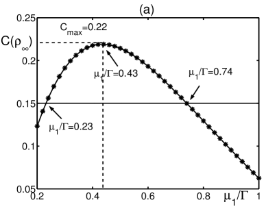
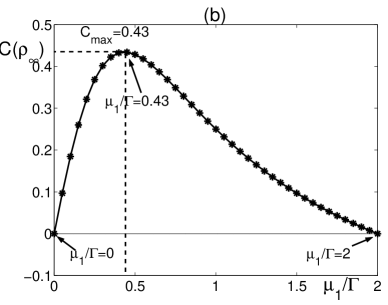
Figure 4: Plots of $C(\rho_{\infty})$ versus $\mu_{1}/\Gamma$ for (a) $\kappa=0.85$, (b) $\kappa=1$. The asterisk line is for the controlled stationary concurrence and the solid line is for the uncontrolled stationary concurrence.

The fact that our strategy is effective only when the parameter $\kappa$ is sufficiently large comes from the competition between $\tilde{\rho}_{m}$ and $\rho_{m}$ in Eq. (20), where $\tilde{\rho}_{m}$ comes from the dissipation effect and $\rho_{m}$ is induced by our proposal. When $\kappa$ is close to $0$, the dissipation dominates and hence the control fails, while, when $\kappa$ is close to $1$, the control becomes effective.

As has been indicated in Sec. 3, the fluctuations of the positions of the atoms would bring an uncertain phase shift for the maximally entangled state $\rho_{m}$, which may deteriorate the stationary concurrence. The calculations are like those in Sec. 3, so we omit them here.

Fig. 5 shows some numerical examples, where the initial states are, respectively,

$$\rho_{0}^{1}=\left(\begin{array}[]{cccc}3/8&&&3/8\\ &1/8&&\\ &&1/8&\\ 3/8&&&3/8\\ \end{array}\right),$$

and

$$\rho_{0}^{2}=\left(\begin{array}[]{cccc}0.85&&&0.1\\ &0.03&&\\ &&0.07&\\ 0.1&&&0.05\\ \end{array}\right).$$

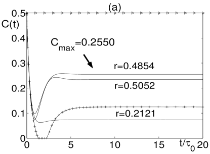
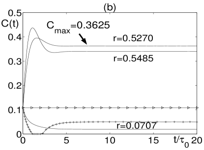
Figure 5: Plots of the concurrence $C(t)$ where the system state is initialized for (a) $\rho_{0}^{1}$ and (b) $\rho_{0}^{2}$. The plus-sign lines denote the uncontrolled trajectories; the triangle lines are for the free trajectories in absence of control and decoherence; the solid lines represent the controlled trajectories with different parameters $r=2\Gamma\mu_{1}\kappa/(\Gamma^{2}+3\mu_{1}^{2})$, which is the proportion of the squeezed field induced maximally entangled state $\rho_{m}$ in Eq. (20).

The simulation results show that the stationary state of the uncontrolled system under the collective amplitude damping decoherence may remain entangled which is quite different from the independent decoherence channel, and this feature has been utilized in the literature [15, 16, 17] to create entanglement between qubits. Our strategy may further increase the entanglement in the stationary entangled state, as shown in comparison between the plus-sign lines and the solid lines.

Another feature of the collective amplitude damping decoherence channel observed from Fig. 5 is that the maximum concurrence depends on the initial state. For certain values of $r$, our control strategy may have worse performance than that induced by the natural dissipation. Both Fig. 5a and 5b provide such a case where the solid line (controlled trajectory) goes below the plus-sign line (uncontrolled trajectory). The corresponding control parameter $\mu_{1}$ is outside the interval given in Eq. (21).

5 Mixed amplitude damping decoherence channel

In actual experiments, the decoherence channel is never perfectly collective, because it is hard to place the two atoms in an cavity close enough. The existing atom trapping and cooling techniques [36, 37] can only hold two atoms approximately at the distance of the same order of the resonant wavelength of the atom. Thus, it is more realistic to treat the resulting decoherence channel as a mixture of an independent amplitude damping decoherence channel and a collective amplitude damping decoherence channel, as shown in the following master equation:

$$\dot{\rho} = -i[H_{A}^{\rm eff},\rho]+\sum_{i=1}^{2}\Gamma\mathcal{D}[\sigma_{-}^{(i)}]\rho+\Gamma_{12}\left(\sigma_{-}^{(1)}\rho\sigma_{+}^{(2)}-\frac{1}{2}\{\sigma_{+}^{(2)}\sigma_{-}^{(1)},\rho\}\right)$$ (24)

$$+\Gamma_{12}\left(\sigma_{-}^{(2)}\rho\sigma_{+}^{(1)}-\frac{1}{2}\{\sigma_{+}^{(1)}\sigma_{-}^{(2)},\rho\}\right),$$

where $0<\Gamma_{12}<\Gamma$.

It can be verified that the stationary state of the uncontrolled system is nothing but the separable two-atom ground state $\rho^{u}_{\infty}=|00\rangle\langle 00|$ in which entanglement completely disappears, as well as in the case of the independent decoherence channel. By introducing the intermediate squeezed field, we can stabilize the system at the same stationary state given in Eq. (10).

6 Conclusions

In summary, we proposed a two-atom entanglement control strategy, via a controllable squeezed field coupled to the two atoms, to protect entanglement from the spontaneous emission process. The parameter amplification coefficient of the squeezed field can be tuned to generate a non-local Hamiltonian, which can be used to maintain entanglement of the two-atom states against decoherence. For the independent amplitude damping decoherence channel, we can partially recover the entanglement of the quantum state which otherwise will be completely lost. For the collective amplitude damping decoherence channel, our strategy can effectively enhance the entanglement of the stationary state compared with the dissipation-induced strategies provided that the uncontrolled stationary state is not tightly entangled.

The proposed entanglement control strategy is an open-loop control strategy, where no measurements are done during the course of control. Such control strategies require exact values of the system parameters, and can badly suffer from the uncertainty of these parameters, which may bring remarkable derivation of the stationary concurrence from the ideal values. This problem is hopefully solvable by quantum feedback controls.

Another direction of the succeeding research will be the application in solid state systems. In such systems, controllable coupling between qubits is easier to be achieved [38, 39] compared with the optical systems. However, interactions between the solid-state systems and their environments are more complicated, which may lead to non-Markovian noises [40]. To what extent the controllable non-local unitary operations can preserve entanglement against non-Markovian noises is an interesting problem to be explored, for which existing decoherence suppression strategies [41, 42, 43] may be helpful.

Appendix A Proof of the Equations (10) and (12)

Firstly, we transform the control model (8) from the complex matrix space into the real vector space, i.e., the so-called coherence vector picture [44, 45, 46, 47]. With respect to the inner product $\langle X,Y\rangle={\rm tr}(X^{\dagger}Y)$, we define the following orthonormal basis for all two-atom operators:

$$\left\{\frac{1}{2}I_{4\times 4},\,\Omega_{14}^{x},\,\Omega_{14}^{y},\,\Omega_{23}^{x},\,\Omega_{23}^{y},\,\frac{1}{2}\sigma_{x}^{(1)},\,\frac{1}{2}\sigma_{y}^{(1)},\,\frac{1}{2}\sigma_{x}^{(2)},\frac{1}{2}\sigma_{y}^{(2)},\,\frac{1}{2}\sigma_{x}^{(1)}\sigma_{z}^{(2)},\right.$$

$$\left.\frac{1}{2}\sigma_{z}^{(1)}\sigma_{x}^{(2)},\,\frac{1}{2}\sigma_{y}^{(1)}\sigma_{z}^{(2)},\,\frac{1}{2}\sigma_{z}^{(1)}\sigma_{y}^{(2)},\,\Omega_{14}^{z},\Omega_{23}^{z},\frac{1}{2}\sigma_{z}^{(1)}\sigma_{z}^{(2)}\right\},$$ (25)

where

$$\Omega_{14}^{x}=\frac{1}{\sqrt{2}}\left(\begin{array}[]{cccc}&&&1\\ &&0&\\ &0&&\\ 1&&&\\ \end{array}\right),\,\,\Omega_{14}^{y}=\frac{1}{\sqrt{2}}\left(\begin{array}[]{cccc}&&&-i\\ &&0&\\ &0&&\\ i&&&0\\ \end{array}\right),$$

$$\Omega_{23}^{x}=\frac{1}{\sqrt{2}}\left(\begin{array}[]{cccc}&&&0\\ &&1&\\ &1&&\\ 0&&&\\ \end{array}\right),\,\,\Omega_{23}^{y}=\frac{1}{\sqrt{2}}\left(\begin{array}[]{cccc}&&&0\\ &&-i&\\ &i&&\\ 0&&&\\ \end{array}\right),$$

$$\Omega_{14}^{z}=\frac{1}{\sqrt{2}}\left(\begin{array}[]{cccc}1&&&\\ &0&&\\ &&0&\\ &&&-1\\ \end{array}\right),\,\,\Omega_{23}^{z}=\frac{1}{\sqrt{2}}\left(\begin{array}[]{cccc}0&&&\\ &1&&\\ &&-1&\\ &&&0\\ \end{array}\right).$$

Under this basis, the system density matrix can be expressed as:

$$\rho=\frac{1}{4}I_{4\times 4}+\sum_{i=1}^{15}m_{i}\Omega_{i},$$

where $m_{i}={\rm tr}(\Omega_{i}\rho)$ and $\Omega_{i},\,i=1,\cdots,15$, are the basis matrices in Eq. (A) except $\frac{1}{2}I_{4\times 4}$. $m=(m_{1},\cdots,m_{15})^{T}$ is called the coherence vector of $\rho$.

In the coherence vector picture, the master equation (8) can be rewritten as [44, 45, 46, 47]:

$$\dot{m}=O_{A}m+Dm+g,$$ (26)

where the orthogonal matrix $O_{A}$ is the adjoint representation [45] of $-iH_{A}^{\rm eff}$. The affine term “$Dm+g$” is that of the Lindblad terms:

$$\Gamma\mathbb{D}[\sigma_{-}^{(1)}]\rho+\Gamma\mathbb{D}[\sigma_{-}^{(2)}]\rho,$$

where $D\leq 0$ and $g$ is a constant vector. Further, divide $m$ into the following sub-vectors:

$$m^{p} = (m_{14}^{x},m_{14}^{y},m_{23}^{x},m_{23}^{y})^{T},$$

$$m^{\eta} = (m_{14}^{z},m_{23}^{z},m_{zz})^{T},$$ (27)

$$m^{\epsilon} = (m_{x0},m_{y0},m_{0x},m_{0y},m_{xz},m_{zx},m_{yz},m_{zy})^{T},$$

where

$$m_{14}^{\alpha}={\rm tr}(\Omega_{14}^{\alpha}\rho),\,m_{23}^{\beta}={\rm tr}(\Omega_{23}^{\beta}\rho),\,\,\alpha,\beta=x,y,z,$$

$$m_{ij}={\rm tr}\left[\left(\frac{1}{2}\sigma_{i}^{(1)}\sigma_{j}^{(2)}\right)\rho\right],\,\,i,j=0,x,y,z,$$

and $\sigma_{0}^{(i)}=I_{2\times 2},\,i=1,2$ are the $2\times 2$ identity operators acting on the $i$-th atom. Then, (26) can be grouped into:

$$\dot{m}^{p} = \sum_{i=1}^{4}u_{i}O_{i}^{\eta}m^{\eta}+D^{p}m^{p},$$

$$\dot{m}^{\eta} = \sum_{i=1}^{4}u_{i}(-O_{i}^{\eta\,T})m^{p}+D^{\eta}m^{\eta}+g^{\eta},$$ (28)

$$\dot{m}^{\epsilon} = \sum_{i=1}^{4}u_{i}O_{i}^{\epsilon}m^{\epsilon}+D^{\epsilon}m^{\epsilon},$$

where

$$u_{1}=8\mu_{1}\cos\phi_{1},\,u_{2}=8\mu_{1}\sin\phi_{1},\,u_{3}=8\mu_{2}\cos\phi_{2},\,u_{4}=-8\mu_{2}\sin\phi_{2},$$

$$D^{p}=-4\Gamma\left(\begin{array}[]{cccc}1&&&\\ &1&&\\ &&1&\\ &&&1\\ \end{array}\right),\,\,O_{1}^{\eta}=\left(\begin{array}[]{ccc}0&0&0\\ -1&0&0\\ 0&0&0\\ 0&0&0\\ \end{array}\right),$$ (37)

$$O_{2}^{\eta}=\left(\begin{array}[]{ccc}1&0&0\\ 0&0&0\\ 0&0&0\\ 0&0&0\\ \end{array}\right),\,\,O_{3}^{\eta}=\left(\begin{array}[]{ccc}0&0&0\\ 0&0&0\\ 0&0&0\\ 0&-1&0\\ \end{array}\right),\,\,O_{4}^{\eta}=\left(\begin{array}[]{ccc}0&0&0\\ 0&0&0\\ 0&1&0\\ 0&0&0\\ \end{array}\right),$$ (50)

$$D^{\eta}=-4\Gamma\left(\begin{array}[]{ccc}1&0&0\\ 0&1&0\\ -\sqrt{2}&0&2\\ \end{array}\right),\,\,g^{\eta}=\left(\begin{array}[]{c}2\sqrt{2}\Gamma\\ 0\\ 0\\ \end{array}\right).$$ (57)

$O_{i}^{\epsilon}$ are all skew-symmetric matrices and $D^{\epsilon}<0$, thereby

$$\frac{d}{dt}((m^{\epsilon})^{T}m^{\epsilon})=(m^{\epsilon})^{T}D^{\epsilon}m^{\epsilon}<0,\quad\forall m^{\epsilon}\neq 0,$$

which implies that $m^{\epsilon}\rightarrow 0$ when $t\rightarrow\infty$.

With simple calculations, the following stationary solution can be obtained for Eq. (A):

$$m^{\epsilon}=0,\,m_{23}^{x}(\infty)=m_{23}^{y}(\infty)=m_{23}^{z}(\infty)=0,$$

$$m_{14}^{x}(\infty)=\frac{\sqrt{2}\mu_{1}\Gamma}{4\mu_{1}^{2}+\Gamma^{2}}\cos\left(\phi_{1}-\frac{\pi}{2}\right),$$

$$m_{14}^{y}(\infty)=\frac{\sqrt{2}\mu_{1}\Gamma}{4\mu_{1}^{2}+\Gamma^{2}}\sin\left(\phi_{1}-\frac{\pi}{2}\right),$$

$$m_{14}^{z}(\infty)=\sqrt{2}m_{zz}(\infty)=\frac{\sqrt{2}\Gamma^{2}}{8\mu_{1}^{2}+2\Gamma^{2}},$$

from which we can obtain the corresponding decomposition (10) of the stationary state $\rho_{\infty}$.

Going back to the density matrix, one can find that the stationary state has the following form:

$$\rho_{\infty}=\left(\begin{array}[]{cccc}a&&&w\\ &b&z&\\ &z^{*}&c&\\ w^{*}&&&d\\ \end{array}\right),$$ (58)

whose concurrence can be analytically solved to be [19, 20, 21]:

$$C(\rho_{\infty})=2\max\{|w|-\sqrt{bc},|z|-\sqrt{ad},0\}.$$ (59)

The above equation leads to the stationary concurrence $C(\rho_{\infty})$ given in Eq. (12).

Appendix B Proof of the Equations (18)–(22)

Similar to what we have done in A, the controlled master equation (17) can be grouped into the following control equations in the coherence vector picture:

$$\dot{m}_{14}^{x} = 8\mu_{1}\sin\theta_{1}m_{14}^{z}-4\Gamma m_{14}^{x},$$

$$\dot{m}_{14}^{y} = -8\mu_{1}\cos\theta_{1}m_{14}^{z}-4\Gamma m_{14}^{y},$$

$$\dot{m}_{14}^{z} = 8\mu_{1}\cos\theta_{1}m_{14}^{y}-8\mu_{1}\sin\theta_{1}m_{14}^{x}-4\Gamma m_{14}^{z}+2\sqrt{2}\Gamma+4\Gamma m_{23}^{x},$$

$$\dot{m}_{23}^{x} = -4\Gamma m_{23}^{x}-4\Gamma m_{14}^{z}+4\sqrt{2}\Gamma m_{zz},$$

$$\dot{m}_{23}^{y} = -8(\mu_{2}+\eta_{0})m_{23}^{z}-4\Gamma m_{23}^{y},$$

$$\dot{m}_{23}^{z} = 8(\mu_{2}+\eta_{0})m_{23}^{y}-4\Gamma m_{23}^{z},$$

$$\dot{m}_{zz} = 4\sqrt{2}\Gamma m_{14}^{z}-8\Gamma m_{zz}+4\sqrt{2}\Gamma m_{23}^{x}.$$ (60)

As well as the independent amplitude damping decoherence model, the sub-vector $m^{\epsilon}=(m_{x0},\cdots,m_{zy})^{T}$ always goes to zero when $t\rightarrow\infty$, and it will not affect $C(\rho_{\infty})$, so we will not discuss $m^{\epsilon}(t)$ here. The fourth and the last equations in Eq. (B) implies a conservation law:

$$m_{zz}(t)+\sqrt{2}m_{23}^{x}(t)\equiv m_{zz}(t_{0})+\sqrt{2}m_{23}^{x}(t_{0})\triangleq 2\kappa-\frac{3}{2}.$$

Substituting $\mu_{1}=\mu_{2}=0$ into Eq. (B), we have the following uncontrolled stationary solution:

$$m_{14}^{x}(\infty)=m_{14}^{y}(\infty)=m_{23}^{y}(\infty)=m_{23}^{z}(\infty)=0,$$

$$m_{14}^{z}(\infty)=\frac{\sqrt{2}}{2}\kappa,\,\,\,m_{23}^{x}(\infty)=\frac{\sqrt{2}}{2}(\kappa-1),\,\,\,m_{zz}(\infty)=\kappa-\frac{1}{2},$$

from which the decomposition (18) can be obtained and $C(\rho^{u}_{\infty})=1-\kappa$.

Further, we can obtain the controlled stationary solution of Eq. (B):

$$m_{14}^{x}(\infty)=\frac{\sqrt{2}\mu_{1}\Gamma\kappa}{\Gamma^{2}+3\mu_{1}^{2}}\cos\left(\phi_{1}-\frac{\pi}{2}\right),\,\,\,m_{14}^{y}(\infty)=\frac{\sqrt{2}\mu_{1}\Gamma\kappa}{\Gamma^{2}+3\mu_{1}^{2}}\sin\left(\phi_{1}-\frac{\pi}{2}\right),$$

$$m_{23}^{y}(\infty)=m_{23}^{z}(\infty)=0,\,\,\,m_{14}^{z}(\infty)=\frac{\sqrt{2}\kappa\Gamma^{2}}{2(\Gamma^{2}+3\mu_{1}^{2})},$$

$$m_{zz}(\infty)=\kappa-\frac{1}{2}-\frac{\mu_{1}^{2}\kappa}{\Gamma^{2}+3\mu_{1}^{2}},\,\,\,m_{23}^{x}(\infty)=\frac{\sqrt{2}}{2}\left(\kappa-1+\frac{\mu_{1}^{2}\kappa}{\Gamma^{2}+3\mu_{1}^{2}}\right),$$

which leads to the decomposition (20). Further, it can be calculated that

$$C(\rho_{\infty})=\max\left\{F_{1}(\mu_{1}),F_{2}(\mu_{2}),0\right\},$$

where

$$F_{1}(\mu_{1})=-\kappa+1+\frac{\mu_{1}^{2}}{\Gamma^{2}+3\mu_{1}^{2}}\kappa-\frac{2\mu_{1}\sqrt{\Gamma^{2}+\mu_{1}^{2}}}{\Gamma^{2}+3\mu_{1}^{2}}\kappa,$$

$$F_{2}(\mu_{1})=\frac{(\Gamma^{2}+2\mu_{1}^{2}+2\Gamma\mu_{1})}{\Gamma^{2}+3\mu_{1}^{2}}\kappa-1.$$

It is easy to verify that $F_{1}(\mu_{1})$ monotonically decreases when the control parameter $\mu_{1}$ increases, thereby

$$F_{1}(\mu_{1})\leq F_{1}(0)=1-\kappa=C(\rho^{u}_{\infty}).$$

Also, we can obtain that

$$F_{2}(\mu_{1})\geq 1-\kappa=C(\rho^{u}_{\infty})\geq 0,$$

when $\mu_{1}$ satisfies Eq. (21). In conclusion, we arrive at

$$C(\rho_{\infty})=F_{2}(\mu_{1})\geq 1-\kappa=C(\rho^{u}_{\infty}).$$

Acknowledgments

The authors would like to thank Dr. Yu-xi Liu for helpful discussions and valuable advice. This research was supported in part by the National Natural Science Foundation of China under Grant Nos. 60704017, 60433050, 60635040, 60674039 and China Postdoctoral Science Foundation. T. J. Tarn would also like to acknowledge partial support from the U.S. Army Research Office under Grant W911NF-04-1-0386.

References

References

• [1] Nielsen M A and Chuang I L 2000 Quantum Computation and Quantum Information (England: Cambridge University Press).
• [2] Einstein A, Podolsky B, and Rosen N 1935 Phys. Rev. 47 777.
• [3] Wootters W K 1998 Phys. Rev. Lett. 80 2245.
• [4] Ren X J, Zhou Z W, Zhou X X, and Guo G C 2008 Phys. Rev. A 77 054302.
• [5] de Vicente J I 2008 J. Phys. A: Math. Theor. 41 065309.
• [6] Hassan A S M and Joag P S 2008 Phys. Rev. A 77 062334.
• [7] Zheng S B and Guo G C 2000 Phys. Rev. Lett. 85 2392.
• [8] Oh S C and Kim J 2006 Phys. Rev. A 73 062306.
• [9] Li F L, Xiong H, and Zubairy M S 2005 Phys. Rev. A 72 010303(R).
• [10] Peskin U, Huang Z, and Kais S 2007 Phys. Rev. A 76 012102.
• [11] Sainz I, Klimov A B, and Roa L 2006 Phys. Rev. A 73 032303.
• [12] Wang J, Wiseman H M, and Milburn G J 2005 Phys. Rev. A 71 042309.
• [13] Carvalho A R R and Hope J J 2007 Phys. Rev. A 76 010301(R).
• [14] Mancini S and Wiseman H M 2007 Phys. Rev. A 75 012330.
• [15] Braun D 2002 Phys. Rev. Lett. 89 277901.
• [16] Plenio M B and Huelga S F 2002 Phys. Rev. Lett. 88 197901.
• [17] Benatti F, Floreanini R, and Piani M 2003 Phys. Rev. Lett. 91, 070402.
• [18] S. Nicolosi, A. Napoli, A. Messina, and F. Petruccione, Phys. Rev. A 70, 022511 (2004).
• [19] Yu T, Eberly J H 2004 Phys. Rev. Lett. 93 140404.
• [20] Yu T, Eberly J H 2006 Phys. Rev. Lett. 97 140403.
• [21] Yu T, Eberly J H 2006 Optics Communications 264 393.
• [22] Almeida M P, de Melo F, Hor-Meyll M, Salles A, Walborn S P, Souto Ribeiro P H, and Davidovich L 2007 Science 316 579.
• [23] Carvalho A R R, Mintert F, Palzer S, and Buchleitner A 2007 Eur. Phys. J. D 41 425.
• [24] Tanas R and Ficek Z 2004 J. Opt. B: Quantum Semiclass. Opt. 6, S610-S617.
• [25] Ficek Z and Tanas R 2002 Phys. Rep. 372, 369.
• [26] Villas-Boas C J, de Almeida N G, Serra R M, and Moussa M H Y 2003 Phys. Rev. A 68 061801(R).
• [27] de Almeida N G, Serra R M, Villas-Boas C J, and Moussa M H Y 2004 Phys. Rev. A 69 035802.
• [28] Blais A, Huang R S, Wallraff A, Girvin S M, and Schoelkopf R J 2004 Phys. Rev. A 69 062320.
• [29] Quadt R, Collett M, and Walls D F 1995 Phys. Rev. Lett. 74 351.
• [30] Boozer A D, Boca A, Miller R, Northup T E, and Kimble H J 2006 Phys. Rev. Lett. 97 083602.
• [31] Pinkse P W H, Fischer T, Maunz P, and Rempe G 2000 Nature 404 365.
• [32] Maunz P, Puppe T, Schuster I, Syassen N, Pinkse P W H, and Rempe G 2004 Nature 428 50.
• [33] Bennett C H, Brassard G, Popescu S, Schumacher B, Smolin J A, and Wootters W K 1996 Phys. Rev. Lett. 76 722.
• [34] Dür W and Briegel H J 2007 Rep. Prog. Phys. 70 1381.
• [35] Duan L M and Guo G C 1998 Phys. Rev. A 58 3491.
• [36] Eichmann U, Bergquist J C, Bollinger J J, Gilligan J M, Itano W M, Wineland D J, Raizen M G 1993 Phys. Rev. Lett. 70 2359.
• [37] DeVoe R G, Brewer R G 1996 Phys. Rev. Lett. 76 2049.
• [38] Liu Y X, You J Q, Wei L F, Sun C P, and Nori F 2005 Phys. Rev. Lett. 95 087001.
• [39] Liu Y X, Wei L F, Tsai J S, and Nori F 2006 Phys. Rev. Lett. 96 067003.
• [40] T. Yu 2004 Phys. Rev. A 69 062107.
• [41] Ganesan N and Tarn T J 2007 Phys. Rev. A 75 032323.
• [42] Zhang M, Dai H Y, Xi Z R, Xie H W, and Hu D W 2007 Phys. Rev. A 76 042335.
• [43] Cui W, Xi Z R, and Pan Y 2008 Phys. Rev. A 77 032117.
• [44] Alicki R and Lendi K 1985 Quantum Dynamical Semigroup and Applications (New York: Springer).
• [45] Altafini C 2003 J. Math. Phys. 44 2357.
• [46] Zhang J, Li C W, Wu R B, Tarn T J, and Liu X S 2005 J. Phys. A: Math. Gen. 38 6587.
• [47] Zhang J, Wu R B, Li C W, Tarn T J, and Wu J W 2007 Phys. Rev. A 75 022324.