On the interaction of the electromagnetic radiation with the breaking plasma waves

Abstract

An electromagnetic wave (EMW) interacting with the moving singularity of the charged particle flux undergoes the reflection and absorption as well as frequency change due to Doppler effect and nonlinearity. The singularity corresponding to a caustic in plasma flow with inhomogeneous velocity can arise during the breaking of the finite amplitude Langmuir waves due to nonlinear effects. A systematic analysis of the wave-breaking regimes and caustics formation is presented and the EMW reflection coefficients are calculated.

I Introduction

A strong interest has persisted in studying the electromagnetic wave (EMW) interaction with the relativistic electron structures represented by electron beams rel-beam , Langmuir waves Photon acceleration ; KrSoob ; Light intensification ; Kando-2007 ; Pirozhkov-2007 ionization fronts Ioniz , relativistic solitons and vortices RelSol in an underdense plasma, and by the oscillating electron layers at a solid target surface OscMir ; Cher ; Naumova .

The laser produced irradiance approaches 10²² W/cm² 1022 , which leads to ultrarelativistic plasma dynamics. By further increasing the irradiance we shall see novel physical regimes such as the radiation friction force dominated EMW-matter interaction RadF . At irradiances around  10²⁸ W/cm² H-E , the focused light becomes so strong that the nonlinear effects come into play, as predicted by quantum electrodynamics, including the vacuum polarization and the electron-positron pair creation from vacuum (see review articles MTB and the liteterature quoted therein). The studies of the EMW interaction with the relativistic structures pave a way towards achieving such the irradiance.

Here we pay the main attention to the “flying mirror” concept Light intensification (see its further development and discussion in Refs. BEKT ; MTB ; RCNP ). The electromagnetic radiation source suggested in this concept has unique advantages. It is robust since it is based on the fundamental process of wave breaking. It enables the control of the output pulse parameters such as frequency, duration, focusing, spectrum, etc., required by a wide range of applications. It allows so high up-shifting of the laser radiation frequency, followed by focusing to a spot whith size determined by the shortened wavelength, that the quantum electrodynamics critical field (Schwinger limit) can be achieved with present-day laser systems Light intensification .

In the “flying mirror” concept, extremely high density thin electron shells in the strongly nonlinear plasma wave, generated in the wake of an ultra-short laser pulse, act as semi-transparent mirrors flying with a velocity close to the speed of light, Fig. 1. The mirrors reflect a counter-propagating pulse, whose frequency is upshifted, duration is shortened and power is increased. The obtained pulse power is proportional to the Lorentz factor $\gamma_{ph}=(1-\beta_{ph}^{2})^{-1/2}$ corresponding to the velocity of the mirrors $v_{ph}=\beta_{ph}c$ while the frequency and the pulse compression are proportional to the square of the Lorentz factor.

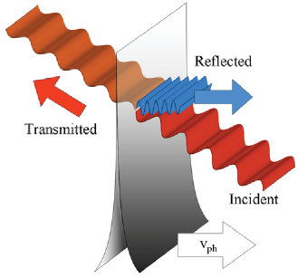
Figure 1: (color online) The “flying mirror” concept. The pulse incident on the moving density cusp is partially reflected. The reflected pulse frequency is upshifted.

A nonlinear wake wave with substantially large amplitude, at which the Lorentz factor of electrons, $\gamma_{e}$, is greater than that of the wake wave, $\gamma_{e}>\gamma_{ph}$, breaks and forms cusps in the electron density distribution Akhiezer-Polovin . It is the steepness of the cusps that affords the efficient reflection of a portion of the counter-propagating laser pulse. If the wake wave is far below the wave-breaking threshold, the reflection is exponentially small. The frequency of the reflected light is upshifted due to the double Doppler effect, as predicted by Einstein Einstein . In his paper, the problem of the reflection of light from a mirror moving with constant velocity, $v_{M}=c\beta_{M}$, close to the speed of light, is solved as an example of the use of relativistic transformations. The incident and the reflected wave frequencies, $\omega_{0}$ and $\omega_{r}$, are related to each other as

$$\omega_{r}=\omega_{0}\frac{1+\beta_{M}^{2}+2\beta_{M}\cos\theta_{0}}{1-\beta_{M}^{2}},$$ (1)

where $\theta_{0}$ is the wave incidence angle. The reflection angle, $\theta_{r}$, is defined by the expression

$$\cos\theta_{r}=\frac{(1+\beta_{M}^{2})\cos\theta_{0}+2\beta_{M}}{1+2\beta_{M}\cos\theta_{0}+\beta_{M}^{2}}.$$ (2)

The wave amplitude transforms according to

$$E_{r}=\mathsf{R}^{1/2}E_{0}\left(\frac{\omega_{r}}{\omega_{0}}\right),$$ (3)

where $\mathsf{R}$ is the reflection coefficient. The role of the moving mirror is played by a steep cusps of the electron density in the wake wave, therefore we write $\beta_{M}=\beta_{ph}=v_{ph}/c$ and $\gamma_{M}=\gamma_{ph}=1/\sqrt{1-\beta_{ph}^{2}}$. The wave propagates in a narrow angle $\Delta\theta\approx 1/\gamma_{M}$. As a result of the interaction with the moving mirror, the reflected electromagnetic pulse is compressed and its frequency is upshifted by a factor which in an ultrarelativistic limit, $\gamma_{ph}\gg 1$, is approximately equal to $4\gamma_{M}^{2}$. It is also conceivable that the interaction of the counter-propagating pulse with the thin relativistic electron shell leads to a higher order harmonic generation, according to a mechanism considered in details in Refs. OscMir ; MTB . The harmonics allow additional compression with the factor $\sim 4n\gamma_{M}^{2}$, where $n$ is a harmonic number.

It is important that the relativistic dependence of the Langmuir frequency on the wave amplitude results in the formation of wake waves with curved fronts that have a form close to a paraboloid D-shape . The paraboloidal mirror focuses the reflected pulse, which results in the intensification of the radiation. In the reference frame moving with the mirror velocity the reflected light has the wavelength equal to $\approx\lambda_{0}/2\gamma_{M}$. It can be focused into the spot with the transverse size $\lambda_{0}/2\gamma_{M}$ with the intensity in the focus given by

$$I_{r}=\mathsf{R}I_{0}\gamma_{M}^{6}\left(\frac{D}{\lambda_{0}}\right)^{2}.$$ (4)

Here $I_{0}$ is the incident wave intensity at the pulse waist $D$.

The flying mirror formed by an electron density modulations in the breaking wake wave can also transform the quasistationary electromagnetic field into a high-frequency short electromagnetic pulse RelSol , such as a low-frequency electromagnetic field of a relativistic electromagnetic sub-cycle soliton, quasistatic magnetic field of an electron vortex, and the quasistationary longitudinal electric field of a wake wave.

The “flying mirror” concept was demonstrated in the proof-of-principle experiments Kando-2007 ; Pirozhkov-2007 , where the narrow-band XUV generation was detected. This opens a way for developing a compact tunable coherent monochromatic X-ray source with the parameters required for various applications in biology, medicine, spectroscopy and material sciencesPirozhkov-2007 .

Reasoning from the principal importance of the nonlinear wake wave dynamics in the “flying mirror” concept, in the present paper we consider a variety of the wake wave breaking regimes. We find typical singularities of the electron density distribution in the breaking wave and calculate their reflection coefficients, $\mathsf{R}$. This provides a key for optimising an operation of the hard electromagnetic radiation source based on the ‘ ‘flying mirror” concept. We describe the EMW interaction with the multiple cusp structure and show the enhancement of the efficiency of the light reflection in this configuration.

II Generic properties of the Wake Wave Breaking

II.1 Gradient catastrophe

The wave breaking in collisionless plasmas provides an example of typical behaviour of the waves in nonlinear systems. The most fundamental properties of nonlinear waves can be represented by Riemann waves in gas dynamics (e.g. see Refs. Z-R ; BBK ), described by the equation

$$\partial_{t}u+w(u)\partial_{x}u=0,$$ (5)

where $u(x,t)$ is the gas velocity and $w(u)=u+c_{s}(u)$. The sound speed $c_{s}(u)$ is a given function of $u$, in a particular case of a cold gas of noninteracting particles it is equal to zero. The solution to Eq. (5) can be written in an implicit form

$$u=U_{0}(x-w(u)t)$$ (6)

with $U_{0}(x)$ being an atrbitrary function deternmined by the initial condition: $u(x)|_{t=0}=U_{0}(x)$. In a finite time the Riemann wave breaks at the location where the gradient of the function $u(x,t)$ becomes infinite. Taking the derivative of the expression (6) with respect to $x$, we obtain

$$\partial_{x}u=\frac{U_{0}^{\prime}(x-w(u))t)}{1+U_{0}^{\prime}(x-w(u)t)w^{\prime}(u)t}.$$ (7)

Here $U_{0}^{\prime}$ and $w^{\prime}$ stand for the derivatives of the functions $U_{0}$ and $w$ with respect to their arguments. For nontrivial dependences of $U_{0}(x)$ and $c_{s}(u)$, we find that the denominator in Eq. (7) vanishes at some point $x_{br}$, i. e. the gradient $u(x,t)$ tends to infinity, at time $t_{br}$ equal to $t_{br}=-1/U_{0}^{\prime}(x_{br}-w(u)t_{br})w^{\prime}(u)$ while the gas velocity $u_{br}=U_{0}(x_{br}-w^{\prime}(u_{br})t_{br})$ remains constant. This phenomenon is known as the “gradient catastrophe” or the “wave breaking”.

Another approach for description of the wave breaking uses a perturbation theory BBK to find the solution to the equation (5). We write

$$u=u^{(0)}+\varepsilon u^{(1)}+\varepsilon^{2}u^{(2)}+\ldots$$ (8)

with $\varepsilon\ll 1$. We assume that in zeroth order the wave amplitude is homogeneous with the velocity, $u^{(0)}$, constant in space and time. To the first order in the wave amplitude, we have

$$\partial_{t}u^{(1)}+w(u^{(0)})\partial_{x}u^{(1)}=0.$$ (9)

This is the simplest wave equation which describes the wave with the frequency and wavenumber related to each other via the dispersion equation $\omega=kw(u^{(0)})$. Thus we obtain the wave propagating in nondispersive media where both the phase velocity, $\omega/k$, and the group velocity, $\partial\omega/\partial k$, are equal to $w(u^{(0)})$. The solution to Eq. (9) is an arbitrary function of the variable $x-w_{0}t$, where $w_{0}=w(u^{(0)})$. We choose it in the form

$$u^{(1)}(X)=u_{m}\sin k(x-w_{0}t).$$ (10)

To the second order in the wave amplitude, we obtain

$$\partial_{t}u^{(2)}-w(u^{(0)})\partial_{x}u^{(2)}=-u^{(1)}w^{\prime}(u^{(0)})\partial_{x}u^{(1)}=$$

$$=-\frac{bk}{2}\sin\left(2k(x-w_{0}t)\right)$$ (11)

with $b=u_{m}^{2}w^{\prime}(u^{(0)})$. The solution to this equation,

$$u^{(2)}(x,t)=-\frac{bkt}{2}\sin\left(2k(x-w_{0}t)\right),$$ (12)

describes the second harmonic with the resonant growth of the amplitude in time.

To the third order in the wave amplitude, we can find that, in general, the amplitude of the the third harmonic grows with time as $t^{2}$, and so on. In the media without dispersion high harmonics are always in resonance with the first harmonic. The resonance between harmonics appears because of the fact that the velocity of propagation is the same for all harmonics; it does not depend on the wave number. This leads to the increase of the velocity gradient (the wave steepenning) linearly with time and to the break of even weak but finite amplitude wave.

The situation with the nonlinear Langmuir wave breaking is different. For simplicity we assume that the wave amplitude is nonrelativistic and the ions are immobile. We cast the equations of the electron fluid motion and the electric field induced in the plasma in the form

$$\partial_{t}v+v\partial_{x}v=-\frac{e}{m_{e}}E,$$ (13)

$$\partial_{t}E+v\partial_{x}E=4\pi en_{0}(\varepsilon x)v.$$ (14)

Here $n_{0}(\varepsilon x)$ with $\varepsilon\ll 1$ is the ion density which is assumed to be weakly inhomogeneous. Although with the use of the Lagrange coordinates a solution to Eqs. (13,14) can be reduced to quadratures, we use a perturbation approach in order to analyse whether or not the high harmonics are in resonance with the first harmonic in the case of nonlinear Langmuir waves. We expand $v(x,t)$, $E(x,t)$, and $n_{0}(\varepsilon x)$ into series:

$$v = \varepsilon v^{(1)}+\varepsilon^{2}v^{(2)}+\ldots,$$

$$E = \varepsilon E^{(1)}+\varepsilon^{2}E^{(2)}+\ldots\ .$$ (15)

In first order from Eqs (13,14) we obtain the equations

$$\partial_{t}v^{(1)}+\frac{e}{m_{e}}E^{(1)}=0,$$ (16)

$$\partial_{t}E^{(1)}-4\pi en_{0}(0)v^{(1)}=0$$ (17)

with the solution

$$v^{(1)}=v_{m}\sin(\omega_{pe}t-kx),$$ (18)

$$E^{(1)}=-\frac{m_{e}v_{m}\omega_{pe}}{e}\cos(\omega_{pe}t-kx),$$ (19)

where $\omega_{pe}=\sqrt{4\pi n_{0}(0)e^{2}/m_{e}}$ is the Langmuir frequency.

The second order in the wave amplitude yields

$$\partial_{t}v^{(2)}+\frac{e}{m_{e}}E^{(2)}=\frac{v_{m}^{2}k}{2}\sin\left(2(\omega_{pe}t-kx)\right),$$ (20)

∂_tE^(2)-4πe n_0(0)v^(2)= (21)

$$=\frac{m_{e}v_{m}^{2}\omega_{pe}k}{2e}\left[1-\cos\left(2(\omega_{pe}t-kx)\right)\right]$$

$$+4\pi en_{0}^{\prime}(0)xv_{m}\sin(\omega_{pe}t-kx).$$

We obtain for $v^{(2)}$ and $E^{(2)}$

$$v^{(2)}=-\frac{v_{m}^{2}k}{2\omega_{pe}}\left[1+\cos 2(\omega_{pe}t-kx)\right]+\frac{n_{0}^{\prime}(0)xv_{m}}{4n_{0}(0)}$$

$$\times\left[2\omega_{pe}t\cos(\omega_{pe}t-kx)-\sin(\omega_{pe}t-kx)\right],$$ (22)

$$E^{(2)}=-\frac{v_{m}^{2}km_{e}}{2e}\sin\left(2(\omega_{pe}t-kx)\right)+\frac{\pi en_{0}^{\prime}(0)xv_{m}}{\omega_{pe}}$$

$$\times\left[2\omega_{pe}t\sin(\omega_{pe}t-kx)-\cos(\omega_{pe}t-kx)\right].$$ (23)

As we see, in the homogeneous plasma, $n_{0}=\mathrm{const}$, there is no a resonance between the modes in the Langmuir wave, in contrast to the Riemann waves considered above. This is due to the difference between the group and the phase velocity of the Langmuir wave: its group velocity in the cold plasma is equal to zero while the phase velocity is finite and is given by the relation $\mathrm{v_{ph}}=\omega_{pe}/k$. The Langmuir wave break occurs if the wave is excited with such a strong amplitude, $v_{0}$, that $v_{0}>\mathrm{v_{ph}}$, out of the applicability of the approximation used in Eqs. (13,14). As seen in Eqs. (II.1,II.1), the breaking occurs also in inhomogeous plasma, where due to the phase mixing effect the wavenumber, $k$, grows with time PhMix .

II.2 Structure of the Breaking Relativistic Wake Wave

In the particular application for the light intensification Light intensification , the characteristic features of the electron density modulations play the key role in the calculating the EMW reflection coefficient.

II.2.1 Wake wave breaking in the relativistic electron beam

We start a discussion of the nonlinear wake wave from the consideration of nonlinear perturbations produced by the laser pulse in the relativistic electron beam. We neglect the space charge effect assuming that the laser pulse — beam interaction can be described in the test particle approximation. The equation for the electron momentum reads

$$\partial_{t}p+v\partial_{x}p=-\frac{m_{e}c^{2}}{2\gamma}\partial_{x}a^{2}.$$ (24)

Here the longitudinal component of the electron velocity, $v$, along the laser pulse propagation direction, is related to the longitudinal component of the electron momentum by $v=p/\gamma m_{e}$; $\gamma=\sqrt{1+a^{2}+\left({p}/{m_{e}c}\right)^{2}}$ is the Lorentz-factor and $a=eE_{0}/m_{e}\omega_{0}c$ is the normalized electric field of the EMW. We assume that the EMW is circularly polarized and depends on the coordinate and time as $a(x-\mathrm{v_{ph}}t)$. The phase velocity of the wake, $\mathrm{v_{ph}}$, equals the laser pulse group velocity, Liu-Ros ; T-D ; Esarey-IEEE . We note that the EMW group velocity, in general, is below the speed of light in vacuum if the laser pulse propagates inside a waveguide, in a plasma, or/and in the focus region (e.g. see Ref. Esarey ). Introducing a new variable

$$\mathrm{X}=x-\mathrm{v_{ph}}t,$$ (25)

we find the integral of Eq. (24)

$$\gamma-\frac{\mathrm{\beta_{ph}}p}{m_{e}c}=h$$ (26)

This integral plays a role of the Hamiltonian in terms of variables ${\rm X}$ and $p$, Fig. 2. with $h$ being a constant and $\mathrm{\beta_{ph}=v}_{ph}/c$. If the laser pulse is of a finite duration and the electron momentum is $p_{0}$ before the interaction with the laser pulse, then the constant $h$ is given by the expression $h=\sqrt{1+\left({p}_{0}/{m_{e}c}\right)^{2}}-\mathrm{\beta_{ph}}p_{0}/m_{e}c$. When the electron is interacting with the laser pulse its velocity is given by the expression

$$v=c\frac{h\mathrm{\beta_{ph}}-\sqrt{h^{2}-(1-\mathrm{\beta_{ph}^{2}})(1+a^{2}({\mathrm{X}}))}}{h-\mathrm{\beta_{ph}}\sqrt{h^{2}-(1-\mathrm{\beta_{ph}^{2}})(1+a^{2}({\mathrm{X}}))}}.$$ (27)

The solution of the continuity equation,

$$\partial_{t}n+\partial_{x}(nv)=0,$$ (28)

gives for the electron density $n=n_{0}(\mathrm{v_{ph}}-v_{0})/(\mathrm{v_{ph}}-v)$, which is equivalent to

$$n=n_{0}\frac{\sqrt{\tilde{h}^{2}-1}}{\tilde{h}-\mathrm{\beta_{ph}}\sqrt{\tilde{h}^{2}-1}}\frac{\tilde{h}-\mathrm{\beta_{ph}}\sqrt{\tilde{h}^{2}-1-a^{2}({\mathrm{X}})}}{\sqrt{\tilde{h}^{2}-1-a^{2}({\mathrm{X}})}}.$$ (29)

Here $v_{0}=cp_{0}/(m_{e}ch+\mathrm{\beta_{ph}}p_{0})$ and

$$\tilde{h}=\frac{h}{\sqrt{1-\mathrm{\beta_{ph}^{2}}}}.$$ (30)

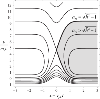
Figure 2: Contours of the Hamiltonian Eq. (26) in the $(x-{\rm v_{ph}}ct,p)$-plane for the Gaussian laser pulse $a({\rm X})=a_{\rm m}\exp(-{\rm X}^{2})$. Shaded region represents trajectories of particles whose initial velocity is in the interval $0\leq v\leq{\rm v_{ph}}$. If the trajectory with $h=1$ is the separatrix, then $a_{\rm m}=\sqrt{\tilde{h}^{2}-1}$, while an enclosed trajectory means $a_{\rm m}>\sqrt{\tilde{h}^{2}-1}$.

At the point $X=X_{br}$, where the denominator in Eq. (29) vanishes, i.e. the electron velocity becomes equal to the phase velocity $\mathrm{v_{ph}}$, the electron density tends to infinity. This corresponds to the breaking of the wave induced by the laser pulse in the electron beam. The threshold corresponding to the lowest amplitude of the laser pulse, at which the pulse piles up the particles towars the infinite density, is determined by the expression

$$a^{2}({\mathrm{X}}_{br})=\tilde{h}^{2}-1.$$ (31)

In the phase plane of the Hamiltonian system described by Eq. (26), the breaking corresponds to $X$-points and to vertical tangents of the contours of the Hamiltonian, Fig. 2.

First, we consider the case when the condition (31) is satisfied precisely at the maximum of the laser pulse amplitude, $a_{\mathrm{max}}=a({\mathrm{X}}_{br})$. In the vicinty of the maximum, the amplitude can be represented by the expansion

$$a({\mathrm{X}})=a({\mathrm{X}}_{br})-\frac{1}{2}a^{\prime\prime}({\mathrm{X}}_{br})\Delta{\mathrm{X}}^{2},$$ (32)

where $\Delta{\mathrm{X=X}}-{\mathrm{X}}_{br}\rightarrow 0$, thus for the electron density, velocity and momentum we obtain

$$n=\frac{\bar{n}_{1}}{|\Delta{\mathrm{X}}|},$$ (33)

$$v=\mathrm{v_{ph}}-\mathrm{\bar{v}_{1}}|\Delta{\mathrm{X}}|,$$ (34)

and

$$p=p_{m}-\bar{p}_{1}|\Delta{\mathrm{X}}|,$$ (35)

respectively. Here

$$\bar{n}_{1}=\frac{n_{0}\tilde{h}a({\mathrm{X}}_{br})}{(\tilde{h}-\mathrm{\beta_{ph}}a({\mathrm{X}}_{br}))\sqrt{a({\mathrm{X}}_{br})a^{\prime\prime}(X_{br})}},$$ (36)

$\mathrm{\bar{v}_{1}}={c(1-\mathrm{\beta_{ph}^{2}})\sqrt{a({\mathrm{X}}_{br})a^{\prime\prime}(X_{br})}}/{\tilde{h}}$,$\ p_{m}=\mathrm{\beta_{ph}}\tilde{h}/\sqrt{1-\mathrm{\beta_{ph}^{2}}}$ and $\bar{p}_{1}=\sqrt{a({\mathrm{X}}_{br})a^{\prime\prime}(X_{br})/\mathrm{(1-\mathrm{\beta_{ph}^{2}})}}$.

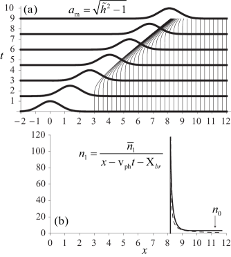
Figure 3: Formation of the density singularity in the beam of particles described by Eq. (24) for the Gaussian laser pulse $a({\rm X})=a_{\rm m}\exp(-{\rm X}^{2})$, $a_{\rm m}=\sqrt{\tilde{h}^{2}-1}$, and $\beta_{\rm ph}=0.9$. (a) Thin lines represent the particle trajectories in the $(x,t)$-plane corresponding to different initial locations of particles in the beam. Thick lines stand for the laser pulse envelope at the corresponding time. (b) The density of the particles at the last moment of time. The dashed line shows the theoretical limit Eq. (33).

The electron motion leading to a pile-up and their density increase is shown in Fig. 3. We note that the singularity in the electron density distribution (33) is not integrable. The integral $\int_{-\Delta{\mathrm{X}}}^{+\Delta{\mathrm{X}}}n(X)dX$ diverges. Formally it takes an infinite time in order to form the singularity. Behavior of the electron density in the vicinity of the breaking point can be described by using the continuity equation (28), the motion integral (26) and the expansion (32). The electron displacement is described by the equation

$$\Delta{\mathrm{\dot{X}}}=v-\mathrm{v}_{ph}=-\mathrm{\bar{v}_{1}}|\Delta\mathrm{X}|$$ (37)

where a dot stands for the total derivative with respect to time. For the initial condition $\Delta{\mathrm{X}}|_{t=0}=\Delta{\mathrm{X}}_{0}$ the solution is

$$\Delta{\mathrm{X}}=\Delta{\mathrm{X}}_{0}\exp(-t/\tau),$$ (38)

where $\tau={\tilde{h}}/{(1-\mathrm{\beta_{ph}^{2}})c\sqrt{a({\mathrm{X}}_{br})a^{\prime\prime}(X_{br})}}$ is the singularity pile-up time. The electron density $n=n_{0}\left|\Delta{\mathrm{X}}_{0}/\Delta{\mathrm{X}}\right|$ at the breaking point grows exponentially: $n=n_{0}\exp(t/\tau)$. Its growth saturates due to a finite number of the electrons in the beam or/and due to the space charge effect. The case when the space charge effect is taken into account is discussed in the next subsection. For a finite number of the particles, the density distribution asimptotically in time can be approximated by

$$n(\mathrm{X})=n_{0}l_{b}\delta({\mathrm{X}}),$$ (39)

where $\delta(x)$ is the Dirac delta function, and $l_{b}$ is the initial length of the bunch.

Apparently, no break occurs for the phase velocity equal to the speed of light in vacuum because the electron velocity is always less than $c$. In this limiting case, $\mathrm{\beta_{ph}=1}$, we have $h=\gamma_{0}-p_{0}/m_{e}c$. The electron Lorentz gamma factor, $\gamma_{0}$, the momentum, $p_{0}$, and the velocity, $v_{0}$, before the interaction with the laser pulse can be written via the constant $h$ as $\gamma_{0}=(1+h^{2})/2h$, $p_{0}=m_{e}c(1-h^{2})/2h$ and $v_{0}=c(1-h^{2})/(1+h^{2})$. Inside the laser pulse the electron acquires $\gamma=\gamma_{0}+a^{2}({\mathrm{X}})/2h$, $p=p_{0}+m_{e}c\ a^{2}({\mathrm{X}})/2h$, and the electron density becomes equal to

$$n=n_{0}\left[1+\frac{a^{2}({\mathrm{X}})}{1+h^{2}}\right].$$ (40)

We see that for the finite amplitude laser pulse the electron density remains to be finite.

Now we consider the case when the laser pulse amplitude is larger than the threshold determined by the condition (31), $a_{\mathrm{max}}>\tilde{h}^{2}-1$. In this case the breaking occurs at the slope of the laser pulse envelope, where the function $a({\mathrm{X}})$ has the expansion

$$a({\mathrm{X}})=a({\mathrm{X}}_{br})-a^{\prime}({\mathrm{X}}_{br})\Delta{\mathrm{X}}.$$ (41)

The local profile of the electron density in the vicinity of the point ${\mathrm{X=X}}_{br}$ is described by

$$n(\mathrm{X})=\bar{n}_{1/2}\frac{\chi({\mathrm{X}})}{\Delta{\mathrm{X}}^{1/2}}.$$ (42)

Here $\chi(x)$ is the unit-step Heviside function ($\chi(x)=0$ for $x<0$ and $\chi(x)=1$ for $x>0$ ) and

$$\bar{n}_{1/2}=\frac{n_{0}\tilde{h}a({\mathrm{X}}_{br})}{(\tilde{h}-\mathrm{\beta_{ph}}a({\mathrm{X}}_{br}))\sqrt{2a({\mathrm{X}}_{br})a^{\prime}(X_{br})}},$$ (43)

At the breaking point the electron momentum becomes equal to $p_{1/2}=\mathrm{\beta_{ph}}\tilde{h}/\sqrt{1-\mathrm{\beta_{ph}^{2}}}$. The particle bounces at this point, starting to move in the same direction as the laser pulse. Its velocity increases from $\mathrm{v}_{ph}$ at ${\mathrm{X=X}}_{br}$ to

$$v_{\infty}=c\left(\frac{\tilde{h}\mathrm{\beta_{ph}}+\sqrt{\tilde{h}^{2}-1}}{\tilde{h}+\mathrm{\beta_{ph}}\sqrt{\tilde{h}^{2}-1}}\right)$$ (44)

for ${\mathrm{X\rightarrow\infty}}$. Asymptotically, the electron density in the reflected beam tends to

$$n=n_{0}\frac{\tilde{h}+\mathrm{\beta_{ph}}\sqrt{\tilde{h}^{2}-1}}{\tilde{h}-\mathrm{\beta_{ph}}\sqrt{\tilde{h}^{2}-1}}.$$ (45)

If the particles are at the rest before interacting with the laser pulse, i.e. $h=1$ and $\tilde{h}=1/\sqrt{1-\mathrm{\beta_{ph}^{2}}}$, then the density in the reflected beam is equal to $n_{0}(1+\mathrm{\beta_{ph}^{2}})/(1-\mathrm{\beta_{ph}^{2}})$. The electron motion demonstrating a bounce of electrons in the ponderomotive potential of the laser pulse and the corresponding compression of the density, as well as the electron pile-up at the breaking point, is shown in Fig. 4.

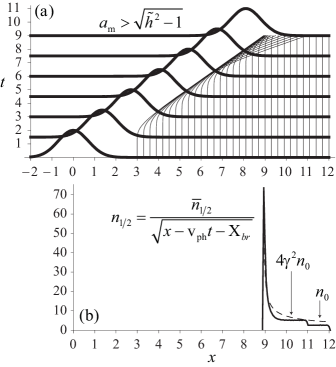
Figure 4: The same graphs as in Fig. 3, but for the two times greater amplitude of the laser pulse, $a_{\rm m}=2\sqrt{\tilde{h}^{2}-1}$. The dashed line in frame (b) shows the main term in the expansion of the density, Eq. (42).

According to Eq. (31) the breaking coordinate depends on the initial electron momentum. For the electron beam with some energy spread it results in a non-trivial electron density distribution in the vicinity of the singularity. We can easily obtain

$$n(\mathrm{X})=\bar{n}_{1/2}\int\limits_{-\infty}^{+\infty}\frac{\chi({\mathrm{X-X}}_{br}(p_{0}))f(p_{0})dp_{0}}{({\mathrm{X-X}}_{br}(p_{0}))^{1/2}}$$ (46)

with $f(p_{0})$ being the distribution function normalized on unity: $\int_{-\infty}^{+\infty}f(p)dp=1$. We assume that the distribution function is given by the ”water bag” model, i.e. $f(p_{0})=\chi(p_{0,T}-|p_{0}|)/2p_{0,T}$, with $p_{0,T}/m_{e}c\ll\mathrm{\beta_{ph}}$. Integration in the right hand-side of Eq. (46) yields

$$n(\mathrm{X})=\frac{\bar{n}_{1/2}}{p_{0,T}}\left[\chi({\mathrm{X-X}}_{br}(-p_{0,T}))\sqrt{{\mathrm{X-X}}_{br}(-p_{0})}\right.$$

$$\left.-\chi({\mathrm{X-X}}_{br}(p_{0,T}))\sqrt{{\mathrm{X-X}}_{br}(p_{0})}\right].$$ (47)

The above consideration is carried out within the framework of the test particle approximation, i.e. neglecting the space charge effect, applicable when the electron density is low enough. We note that the space charge effects are negligible in the electron-positron plasmas because the electron and positron has equal absolute walues of the charge and mass.

Another important case when one can neglect the space charge effects is the limit of extremely high EMW intensity in the so-called “radiation pressure dominated regime” (for details see Refs. RadF ; TZE ; FB ) briefly considered in Appendix A.

II.2.2 The plasma wake wave breaking

Here we discuss the generic properties of the breaking of the Langmuir waves in plasmas. We shall consider the case when the wake wave is excited by a high intensity laser pulse Liu-Ros ; T-D ; GK . This consideration is relevant to the breaking of the wake wave excited by the ultrarelativistic electron bunch Chen . Within the framework of one-dimensional approximation, the relativistic Langmuir wave excitation by the electromagnetic wave can be described by the equation for the electron momentum, $p$,

$$\partial_{t}p+v\partial_{x}p=-eE-\frac{m_{e}c^{2}}{2\gamma}\partial_{x}a^{2}.$$ (48)

In contrast to Eq. (24), it incorporates the space charge effects via the term with the electric field, $E$, for which we have the equation

$$\partial_{t}E+v\partial_{x}E=4\pi en_{0}ev.$$ (49)

Left in a plasma behind a finite width laser pulse, the Langmuir wave has the period $T_{wf}={2\pi}/{\omega_{pe}}=\sqrt{{m_{e}}/{2ne^{2}}}$, in the limit of small amplitude, ${p_{m}}/{m_{e}c}\rightarrow 0$. In the opposite limit of a large amplitude, ${p_{m}}/{m_{e}c}\gg 1$, the wake wave period is $T_{wf}=4\sqrt{2p_{m}/m_{e}c}/{\omega_{pe}}$. Here the maximum wave amplitude, $p_{m}$, is related to the laser pulse amplitude as $p_{m}=m_{e}c{a^{2}}/2$. Therefore, the wakefield wavelength $\lambda_{wf}\approx cT\propto a$ is proportional to the laser pulse amplitude.

For the laser pulse propagating with constant phase velocity $\mathrm{v_{ph}}$, we seek a solution of Eqs. (48,49) in the form of a progressive wave, when the solution depends on the variables $t$ and $x$ in the combination (25). As a result we obtain the ordinary differential equation

$$\left(\gamma-\frac{p}{m_{e}c^{2}}\mathrm{v_{ph}}\right)^{\prime\prime}=\frac{\omega_{pe}^{2}}{c^{2}}\frac{p}{\gamma m_{e}\mathrm{v_{ph}}-p},$$ (50)

where the prime denotes a derivative with respect to $\mathrm{X}$. For piecewise-constant profiles of $a({\mathrm{X}})$, a solution of Eq. (50) can be expressed in terms of elliptic integrals. Here we analyze the solutions of this equation in the vicinity of the singularity. The right hand side of Eq. (50) becomes singular when the denominator, $\gamma m_{e}\mathrm{v_{ph}}-p$, tends to zero, i.e when the electron velocity $v$ becomes equal to the pase velocity of the wake wave, $\mathrm{v_{ph}}$. In the stationary wake wave, the singularity is reached at the maximum value of the electron velocity, $v_{m}={p_{m}}/{\gamma_{m}m_{e}}$, at $\mathrm{X}=\mathrm{X}_{m}$. This singularity, called also the “gradient catastrophe”, corresponds to the wave breaking. In other words, the Langmuir wave breaks when the electric field $E_{wf}$ is above the Akhiezer-Polovin electric field $E_{A-P}=(m_{e}\omega_{pe}c/e)\sqrt{2(\gamma_{ph}-1)}$ with $\gamma_{ph}=1/\sqrt{1-\mathrm{\beta_{ph}^{2}}}$, which means that the electron displacement inside the wave becomes equal to or larger than the wavelength of the wake plasma wave (see Ref. Akhiezer-Polovin ).

In order to find the singularity structure we expand the electron momentum, $p$, and the Lorentz factor, $\gamma$, in the vicinity of their maximum, $\Delta\mathrm{X}=\mathrm{X}-\mathrm{X}_{m}\rightarrow 0$. The momentum is represented by

$$p=p_{m}+\delta p+O(\delta p^{2}),$$ (51)

with

$$p_{m}=m_{e}c\mathrm{\beta_{ph}}\sqrt{\frac{1+a_{m}^{2}}{1-\mathrm{\beta_{ph}^{2}}}}$$ (52)

and $|\delta p/p_{m}|\ll 1$. Here $a_{m}=a({\mathrm{X}_{m}})$. Keeping the main terms of expansions over $\delta p$ in both sides of Eq. (50), we obtain

$$\left(\delta p^{2}\right)^{\prime\prime}=-\varkappa^{2}\frac{1}{\delta p}$$ (53)

with $\varkappa^{2}=2\mathrm{\beta_{ph}}\gamma_{\mathrm{ph}}^{6}(1+a_{m}^{2})\omega_{pe}^{2}m_{e}^{3}c$. Multiplying the left- and right-hand sides of Eq. (53) on $(\delta p^{2})^{\prime}$ and integrating over ${\mathrm{X}}$, we obtain

$$\delta p\delta p^{\prime}=\sqrt{m_{e}^{2}c^{2}f^{2}-\varkappa^{2}\delta p},$$ (54)

where $f$ is an integration constant. We note that since Eq. (53) has singularity due to the initial condition $\left.\delta p\right|_{\Delta\mathrm{X}=0}=0$, in principle, one can choose different values for the integration constant in different intervals with boundary $\Delta\mathrm{X}=0$, i. e. $f=f^{-}$ in the interval $\Delta\mathrm{X}<0$ and $f=f^{+}\not=f^{-}$ for $\Delta\mathrm{X}>0$. The behavior of the function $\delta p({\mathrm{X}})$ at the singularity is different depending on the behaviour of the product $\delta p\delta p^{\prime}$ at $\delta p\rightarrow 0$.

If the product $\delta p\delta p^{\prime}$ is finite and nonzero for $\delta p\rightarrow 0$, then the main term in the expansion of the solution of Eq. (54) at $\Delta\mathrm{X}\rightarrow 0$ is

$$\delta p=-m_{e}c\sqrt{2f|\Delta{\mathrm{X}}|}.$$ (55)

Using this expression we find the electron velocity:

$$v\approx\mathrm{v_{ph}}-\frac{c}{\gamma_{ph}^{3}}\left(\frac{2f|\Delta{\mathrm{X}}|}{1+a_{m}^{2}}\right)^{1/2}$$ (56)

The electron density, $n(\mathrm{X})$, is given by the solution to the continuity equation (28). In the vicinity of the singularity it reads

$$n=\frac{n_{0}\mathrm{v_{ph}}}{\mathrm{v_{ph}}-v}\approx n_{0}\mathrm{\beta_{ph}}\gamma_{ph}^{3}\left(\frac{1+a_{m}^{2}}{2f|\Delta{\mathrm{X}}|}\right)^{1/2}.$$ (57)

If at $\delta p\rightarrow 0$, $\delta p\delta p^{\prime}\rightarrow 0$, which means $f=0,$ then the main term in the expansion of the solution of Eq. (54) at $\Delta\mathrm{X}\rightarrow 0$ reads

δp= -(32ϰΔX)^2/3 = (58)

$$=-m_{e}\mathrm{\beta_{ph}}\gamma_{ph}^{3}\left(\frac{3\omega_{pe}\sqrt{1+a_{m}^{2}}}{\sqrt{2}\mathrm{\beta_{ph}}}\Delta{\mathrm{X}}\right)^{2/3}$$

For the electron velocity we obtain

$$v\approx\mathrm{v_{ph}}-\frac{\mathrm{v_{ph}}}{\gamma_{ph}}\left(\frac{3\omega_{pe}(1+a_{m}^{2})^{1/4}}{\sqrt{2}\mathrm{\beta_{ph}}}\Delta{\mathrm{X}}\right)^{2/3}$$ (59)

In the vicinity of the singularity the electron density distribution is given by

$$n=\frac{n_{0}\mathrm{v_{ph}}}{\mathrm{v_{ph}}-v}\approx n_{0}\gamma_{ph}\left(\frac{\sqrt{2}(1+a_{m}^{2})^{1/4}\mathrm{\beta_{ph}}}{3\omega_{pe}\Delta{\mathrm{X}}}\right)^{2/3}$$ (60)

We found three types of the singularity which appears in the electron density due to wave breaking. In each case the singularity corresponds to the caustic in the plasma flow with inhomogeneous velocity. General description evoking geometric properties of the hydrodynamic flow, presented in Appendix B, shows that the electron density singularity can be approximated by the dependence $n({\mathrm{X}})\propto({\mathrm{X}-\mathrm{X}_{m}})^{-\alpha}$ with $1/2\leq\alpha<1$.

III Electromagnetic wave reflection at the crest of the breaking wake

As we discussed in Introduction, the “flying mirror” concept proposed in Ref. Light intensification makes use of the wave breaking occuring in wake waves generated in a subcritical plasma by an ultrashort laser pulse (further called “driver”). In a strongly nonlinear wake wave, the electron density is modulated in such a way that the electrons form relatively thin layers moving with the velocity $v_{ph}$. A counter-propagating laser pulse (called “signal”) interacts with the plasma, perturbed by the driver. Under certain conditions, the signal is partially reflected from the wake wave, which thereby plays the role of a relativistic mirror. As the wake wave amplitude approaches the threshold for wave breaking (i.e., when the electron velocity in the wave approaches its wave phase velocity), the electric field profile in the wave steepens and, correspondingly, the singularity is formed in the electron density profile. It is important that the singularity affords partial reflection of the signal with some reflection coefficient $\mathsf{R}$. As shown in Appendix B, in general, the singularity can be represented as $n({\mathrm{X}})\propto({\mathrm{X}-\mathrm{X}_{m}})^{-\alpha}$, $1/2\leq\alpha<1$. Although the singularity is integrable for $\alpha<1$, it breaks the geometric optics approximation and leads to the efficient reflection of a portion of the radiation accompanied by the upshifting of the frequency of the reflected pulse. When $\alpha\rightarrow 1$, the modulation of the electron density is so strong that the reflection coefficient becomes to be of the order of unity.

In order to calculate the reflection coefficient, we consider the interaction of an electromagnetic wave, representing the signal, with a singularity of the electron density formed in a breaking Langmuir wave. The electromagnetic wave, given by the $z$-component of the vector potential $A_{z}(x,y,t)$, is described by the wave equation

$$\partial_{tt}A_{z}-c^{2}(\partial_{xx}A_{z}+\partial_{yy}A_{z})+\omega_{pe}^{2}(x-\mathrm{v_{ph}}t)A_{z}=0,$$ (61)

where $\omega_{pe}^{2}({\mathrm{X}})=4\pi e^{2}n({\mathrm{X}})/m_{e}\gamma$ and the electron Lorentz factor, $\gamma$, is equal to $\gamma_{ph}$ at the point where the density, $n(X)$, is maximum.

III.1 The case $n({\mathrm{X}})\propto{\mathrm{X}}^{-\alpha}$ with $\alpha<1$

Here we consider the general case of the singularity formed in the electron density at the point of the wake wave breaking, which is defined by

$$n({\mathrm{X}})=\frac{n_{0}G_{\alpha}}{(k_{p}\mathrm{X})^{\alpha}},$$ (62)

where $G_{\alpha}=\mathrm{const}$ is the dimensionless constant, $1/2\leq\alpha<1$.

In the boosted reference frame, moving with the phase velocity of the Langmuir wave, the equation (61) takes the form

$$\frac{d^{2}a(\zeta)}{d\zeta^{2}}+\left(s^{2}-\frac{g_{\alpha}}{|\zeta|^{\alpha}}\right)a(\zeta)=0$$ (63)

with

$$a(\zeta)=\frac{eA_{z}(\zeta)}{m_{e}c^{2}}\exp(-i({\omega}^{\prime}{t}^{\prime}-{k}_{y}{y}))$$ (64)

and

$$g_{\alpha}=G_{\alpha}k_{p}^{2-\alpha}\gamma_{ph}^{\alpha-1}.$$ (65)

Here

$$s^{2}=(\omega^{\prime}/c)^{2}-k_{y}^{2}>0,$$ (66)

and $\zeta=(x-\mathrm{v_{ph}}t)\gamma_{\mathrm{ph}}$, ${t}^{\prime}$, ${k}^{\prime},{\omega}^{\prime}$ are the coordinates and time and the wave vector and frequency in the boosted frame. According to Eqs. (60), (65), the coefficient $g_{\alpha}$ for $\alpha=2/3$ is equal to

$$g_{2/3}\approx({2}/{9})^{1/3}(1+a_{m}^{2})^{1/6}k_{p}^{4/3}\gamma_{ph}^{2/3},$$ (67)

i.e. $G_{2/3}=({2}/{9})^{1/3}(1+a_{m}^{2})^{1/6}\gamma_{ph}$.

WKB-approximation gives asymptotic solutions of Eq. (63) for large $|s|$ and $|\zeta|$

$$a(\zeta) \approx W_{1}(\zeta)\left\{\tau\,e^{isW(\zeta)}+\rho\,e^{-isW(\zeta)}\right\},$$ (68)

$$W(\zeta) = \int\limits_{\zeta_{0}}^{\zeta}\sqrt{1-\frac{g_{\alpha}}{s^{2}|\zeta|^{\alpha}}}d\zeta,$$ (69)

$$W_{1}(\zeta) = \left(1-\frac{g_{\alpha}}{s^{2}|\zeta|^{\alpha}}\right)^{-1/4},$$ (70)

where $\tau$ and $\rho$ are constant.

We are interested in solutions such that for $\zeta\rightarrow+\infty$, $\tau$ represents the amplitude of the incident wave (assumed to be equal to 1) and $\rho$ is the reflected wave amplitude, while in the opposite limit, $\zeta\rightarrow-\infty$, $\tau$ stands for the transmitted wave and $\rho$ vanishes. Consequently, we write:

$$\tau(+\infty)=1,\quad|\rho(+\infty)|^{2}=\mathsf{R},$$ (71)

$$|\tau(-\infty)|^{2}=\mathsf{T},\quad\rho(-\infty)=0,$$ (72)

where we assume that the reflection is small,

$$\mathsf{R}\rightarrow 0\ \quad\mathrm{and}\quad\mathsf{T}\rightarrow 1\quad\mathrm{at}\quad s\rightarrow\infty.$$ (73)

We multiply Eq. (63) by $da(\zeta)/d\zeta$, integrate it over $\zeta$ and obtain

$$\left.\left[\left(\frac{da(\zeta)}{d\zeta}\right)^{2}+s^{2}a^{2}(\zeta)\right]\right|_{\zeta_{1}}^{\zeta_{2}}=\int\limits_{\zeta_{1}}^{\zeta_{2}}\frac{g_{\alpha}}{|\zeta|^{\alpha}}\frac{da^{2}(\zeta)}{d\zeta}d\zeta\,.$$ (74)

According to Eq. (68), at large $|s|$ and $|\zeta|$ we have

(da(ζ)dζ) ^2+s^2a^2(ζ)≈4s^2τρ (75)

$$+\frac{g_{\alpha}}{|\zeta|^{\alpha}}\left[\tau^{2}e^{2isW(\zeta)}+\rho^{2}e^{-2isW(\zeta)}\right].$$

Using Eq. (71), (72), we obtain

$$\mathsf{R}_{\alpha}=\frac{1}{4s^{2}}\left.\left[\left(\frac{da(\zeta)}{d\zeta}\right)^{2}+s^{2}a^{2}(\zeta)\right]\right|_{-\infty}^{\infty}=$$

$$\frac{g_{\alpha}}{4s^{2}}\int\limits_{-\infty}^{+\infty}\frac{1}{|\zeta|^{\alpha}}\frac{da^{2}(\zeta)}{d\zeta}d\zeta.$$ (76)

Where the main term in the integrand in the right hand side of Eq. (76) for large $s$ is

$$\frac{1}{|\zeta|^{\alpha}}\frac{da^{2}(\zeta)}{d\zeta}\approx\frac{2isW_{1}^{2}(\zeta)\exp(2isW(\zeta))}{|\zeta|^{\alpha}}\approx$$

$$\approx\frac{2is}{|\zeta|^{\alpha}}\exp\left(2is\zeta-\frac{ig_{\alpha}\zeta^{1-\alpha}}{(1-\alpha)s}\right).$$ (77)

This approximation fails in an interval around $\zeta=0$. The interval size decreases at large $s$ and small $g_{\alpha}$ thus the intergration over this interval yields negligibly small contribution to the reflection coefficient. Neglecting $s^{-1}$-term in the exponent in Eq. (77), we obtain

$$\mathsf{R}_{\alpha}=\frac{ig_{\alpha}\Gamma(1-\alpha)}{2^{1-\alpha}s^{2-\alpha}}\sin\left(\frac{\pi\alpha}{2}\right),$$ (78)

where $\Gamma$ is the Gamma function A-S . For $\alpha=1/2$, this coefficient is

$$\mathsf{R}_{1/2}=\frac{i\pi^{1/2}g_{1/2}}{2s^{3/2}}.$$ (79)

For $\alpha=2/3$, this coefficient is

$$\mathsf{R}_{2/3}=\frac{i3^{1/2}\Gamma(1/3)g_{2/3}}{(2s)^{4/3}}.$$ (80)

For $\alpha\rightarrow 1$ and fixed $s$ and $g_{\alpha}$, the main term in the expansion of the coefficient (78) over $(1-\alpha)$ is $\mathsf{R}_{\alpha}\approx ig_{\alpha}s^{-1}(1-\alpha)^{-1}$. The above used approximation implies a smallness of the relection coefficient compared to unity, i.e. the condition $s\gg(1-\alpha)^{-1}$ must be fulfilled. In the case $\alpha=1$, which requires special consideration, this condition can not be satisfied. The case $\alpha=1$ is analysed below.

III.2 The case $n({\mathrm{X}})\propto{\mathrm{X}}^{-1}$

Here we consider the problem of EMW reflection at the following electron density profile

$$n({\mathrm{X}})=\frac{n_{0}G_{1}}{k_{p}|\mathrm{X}|}.$$ (81)

Since this singularity is non-integrable, the thin layer approximation is not applicable. As stated above, this profile formally requires an infinite number of electrons and its formation takes an infinite time. We use the standard matching technique. Substituting $\alpha=1$ to Eq. (63) we obtain the equation

$$\frac{d^{2}a(\zeta)}{d\zeta^{2}}+\left(s^{2}-\frac{g_{1}}{|\zeta|}\right)a(\zeta)=0$$ (82)

where $\zeta$ is the coordinate in the boosted frame of reference and $g_{1}$ is defined by Eqs. (65. The solution to this equation can be expressed in terms of the confluent hypergeometric functions of the first, $M(a,b,z)$, and the second kind, $U(a,b,z)$, also known as the Kummer’s function of the first and second kind A-S :

$$a_{+}(\zeta) = ie^{-is\zeta}\left[\frac{-c_{1}^{+}}{g_{1}\Gamma\left({ig}_{1}/{2s}\right)}U\left(-\frac{ig_{1}}{2s},0,2is\zeta\right)\right.$$ (83)

$$\left.+c_{2}^{+}\zeta M\left(1-\frac{ig_{1}}{2s},2,2is\zeta\right)\right]$$

in the region $\zeta>0$ and

$$a_{-}(\zeta) = ie^{-is\zeta}\left[\frac{c_{1}^{-}}{g_{1}\Gamma\left({-ig}_{1}/{2s}\right)}U\left(\frac{ig_{1}}{2s},0,2is\zeta\right)\right.$$ (84)

$$\left.+c_{2}^{-}\zeta M\left(1+\frac{ig_{1}}{2s},2,2is\zeta\right)\right]$$

for the negative coordinate $\zeta<0$. These functions should be equal to each other at $\zeta=0$ for all $s$, i.e.

$$a_{+}(+0)-a_{-}(-0)=\frac{(c_{1}^{+}-c_{1}^{-})}{\pi g_{1}}\sinh\left(\frac{\pi g_{1}}{2s}\right)=0,$$ (85)

which entails $c_{1}^{-}=c_{1}^{+}$. The derivatives of $a_{+}(\zeta)$ and $a_{-}(t)$ with respect to $\zeta$ should differ at $\zeta=0$ for all $s$ by

$$a_{+}^{\prime}(+0)-a_{-}^{\prime}(-0) = V.P.\int\limits_{-\varepsilon}^{+\varepsilon}\frac{a(\zeta)}{|\zeta|}\,d\zeta=$$ (86)

$$= \frac{2c_{1}^{+}}{\pi}\ln(\varepsilon)\sinh\left(\frac{\pi g_{1}}{2s}\right).$$

It yields

$$c_{2}^{-}=c_{2}^{+}-c_{1}^{+}\sinh\left(\frac{\pi g_{1}}{2s}\right)\left[1+id(s)\right],$$

where

$$d(s)= \frac{1}{\pi}\Big{[}4\mathbf{\gamma}_{\mathrm{E-M}}+2\log\left({2s}\right)\Big{.}$$ (87)

$$\Big{.}+\psi\left(1-\frac{ig_{1}}{2s}\right)+\psi\left(1+\frac{ig_{1}}{2s}\right)\Big{]},$$

is real monotonously growing function for $g_{1}>0$ and $s>0$, $\mathbf{\gamma}_{\mathrm{E-M}}=0.577...$ is the Euler-Mascheroni constant and $\psi(z)$ is the digamma function A-S .

The series expansions of both the branches, (83) and (84), at $\zeta\rightarrow\pm\infty$ contain the terms proportional to $\exp{(is\zeta)}$ and $\exp{(-is\zeta)}$. The positive exponent corresponds to the incident and transmitted wave, while the negative exponent – to the reflected wave. Obviously there is no reflected wave behind the singularity at $\zeta\rightarrow-\infty$, i.e. the term in $a_{-}(\zeta)$ proportional to $\exp{(-is\zeta)}$ should vanish. As a result we find a relationship between $c_{2}^{+}$ and $c_{1}^{+}$:

$$c_{2}^{+}=c_{1}^{+}\!\left[\cosh\left(\frac{\pi g_{1}}{2s}\right)+i\sinh\left(\frac{\pi g_{1}}{2s}\right)d(s)\right].$$ (88)

Now we can find the amplitudes of the reflected, $\rho$, and transmitted, $\tau$, waves as the ratios of the reflected-to-incident and transmitted-to-incident waves, respectively:

ρ(s)=Γ(-ig1/2s)Γ(ig1/2s)( 2s)^i g_1/s (89)

$$\times\left[1-\frac{\exp(-\pi g_{1}/2s)}{\cosh(\pi g_{1}/2s)+i\sinh(\pi g_{1}/2s)d(s)}\right],$$

τ(s)=-Γ(-ig1/2s)Γ(ig1/2s)(2s)^i g_1/s (90)

$$\times\frac{\exp(-\pi g_{1}/s)}{\cosh(\pi g_{1}/2s)+i\sinh(\pi g_{1}/2s)d(s)}.$$

The reflection coefficient is

$$\mathsf{R}_{1}=|\rho|^{2}=1-\frac{1}{\cosh^{2}(\pi g_{1}/2s)+d(s)^{2}\sinh^{2}(\pi g_{1}/2s)},$$ (91)

the transmission coefficient is

$$\mathsf{T}_{1}=|\tau|^{2}=\frac{\exp(-2\pi g_{1}/s)}{\cosh^{2}(\pi g_{1}/2s)+d(s)^{2}\sinh^{2}(\pi g_{1}/2s)},$$ (92)

We note that for the density profile $n\propto|{\zeta}|^{-1}$ the sum of the reflection and transmission coefficients is less than one, $\mathsf{R}_{1}+\mathsf{T}_{1}=|\rho|^{2}+|\tau|^{2}<1$. This corresponds to a partial absorbtion of the wave energy in the region of the singularity, similarly to the case $n\propto{\zeta}^{-1}$ anylized in Refs. Budden and Stix . The dependence of the reflection, transmission and absorption, $\mathsf{A}_{1}=1-\mathsf{R}_{1}-\mathsf{T}_{1}$, coefficients on the wave number, $s$, is shown on Fig. 5.

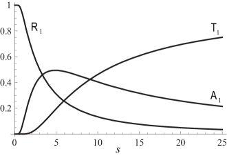
Figure 5: Coefficients of reflection ($\mathsf{R}_{1}=\rho^{2}$), transmission ($\mathsf{T}_{1}=\tau^{2}$), and absorbtion ($\mathsf{A}_{1}=1-\mathsf{R}_{1}-\mathsf{T}_{1}$) as functions of the wave number $s$ for the case $n(\mathrm{X})\propto\mathrm{X}^{-1}$ .

IV Laser pulse interaction with multiple relativistic mirrors

A number of the photons reflected at the semi-transparent mirror depends on the regime of nonlinear wake wave breaking. In Refs. KrSoob ; Pirozhkov-2007 ; BEKT ; MTB and above it is shown that although the reflection coefficient is small, it is not exponentially smal. For example, in the case of typical singularity with $n({\mathrm{X}})\propto{\mathrm{X}}^{-2/3}$ the reflection coefficient in the boosted frame of reference is $\mathsf{R}\approx 1/2\gamma_{M}^{3}$, i.e. a number of photons reflected at a single breaking wake is $\delta N_{ph}\approx N_{s,ph}/2\gamma_{M}^{3}$. Here $N_{s,ph}$ is a number of photons in the incident (signal) pulse.

There is a way to increase the number of reflected photons by using multiple wake wave periods with the electron density singularity in each period. Such the configuration is typically formed behind the ultrashort laser pulse in the underdense plasma. It is easy to show that when the pulse interacts with a train of wake waves, the number of reflected photons is given by the sum

$$N_{r,ph}=N_{s,ph}r\sum_{i=0}^{\mathcal{N}_{w}}(1-\mathsf{R})^{i}=N_{s,ph}\left[1-(1-\mathsf{R})^{\mathcal{N}_{w}}\right].$$ (93)

Here $\mathcal{N}_{w}$ is a number of the wake wave periods. Then the energy of the reflected electromagnetic radiation is

$$\mathcal{E}_{r}=\mathcal{E}_{s}\left(\frac{1+\beta_{M}}{1-\beta_{M}}\right)\left[1-(1-\mathsf{R})^{\mathcal{N}_{w}}\right].$$ (94)

In the limit $\mathsf{R}\mathcal{N}_{w}\ll 1$, we have $N_{r,ph}\approx N_{s,ph}\mathsf{R}\mathcal{N}_{w}$, with the reflected electromagnetic energy given by

$$\mathcal{E}_{r}\approx(4\mathsf{R}\mathcal{N}_{w}/\gamma_{M})\mathcal{E}_{s}.$$ (95)

In the limit $\mathcal{N}_{w}\rightarrow\infty$, the reflected back energy equals to

$$\mathcal{E}_{r}=4\gamma_{M}^{2}\mathcal{E}_{s}.$$ (96)

We see that the energy of the reflected pulse can be many times greater than that of the incident pulse. The energy gain is due to the momentum transfer from the wake wave to the reflected radiation.

Under conditions which are expected to be realized in a moderate intensity laser — gas target interaction, the plasma inhomogeneity can play an important role. If the driver pulse normalized amplitude, $a=eE/m_{e}\omega c$, is not large enough to excite the breaking wake wave, i.e. $a^{2}<2\gamma_{ph}$, the wave reaches the breaking threshold due to growth of its wave number. As well known, the Langmuir waves belong to a class of the waves with continuous frequiency spectrum. In inhomogeneous medium the wave vector, $\mathbf{k}_{p}$ , and wave frequency, $\omega_{p}$, are related to each other via the equation

$$\partial_{t}\mathbf{k}_{p}=-\nabla\omega_{p}.$$ (97)

The frequency dependence on the coordinates can also be due its dependence on the wave amplitude in the case of transversally inhomogeneous laser pulse driver, which is typical for the laser plasma interaction. As a result, the wake wave breaks when $\omega_{p}/|\mathbf{k}_{p}|\approx v_{e}$, i.e. when the wave phase velocity, $\omega_{p}/|\mathbf{k}_{p}|$, becomes equal to the electron quiver velocity $v_{e}$ (for details see Refs. PhMix ). In this regime the breaking wake wave gamma factor, $\gamma_{ph}$, is determined not by the plasma density, but by the driver laser pulse amplitude, and it is equal to $\gamma_{e}$.

V Conclusion

The plasma wave breaking leads to the formation of moving caustics in the plasma flow, which correspond to singularities of the particles distribution in the phase space. The singularity structure depends of the breaking conditions determined by the parameters of plasma and the driver laser pulse which excites the plasma wave. We found the structure of typical singularities appearing in the plasma particle density during the wave breaking. The singularity in the electron density, moving along with the wake wave, acts as a flying relativistic mirror for the counter-propagating electromagnetic radiation, reflecting the light and up-shifting its frequency. Such the reflection results in generation of an ultra-intense electromagnetic radiation. We found the coefficients of the reflection of an electromagnetic wave at the singularities (crests) of the electron density piled up in the most typical regimes of strongly nonlinear wave breaking in collisionless plasmas. Although the reflection coefficients are small, they are not exponentially small, as it is usual in the geometric-optic approximation of the over-barrier reflection from the electron density modulations, applicable for the wake wave far below the breaking threshold. The efficiency of the photon reflection can be substatially increased by using the regimes providing high order sigularity formation (see Eq. (78) or by realizing the laser pulse reflection from several subsequent density singularities, which can be naturally produced in the long enough wake wave. We show that in the multiple-mirror configuration, the energy of the counter-propagating laser pulse reflected back and pumped by the wake wave can be increased by the factor of $4\gamma_{M}^{2}$. This paves a way towards producing high efficiency compact sources of hard electromagnetic radiation.

Asknowledgments

This work was supported in part by the Japanese Ministry of Education, Science, Sports and Culture, Grant-in-Aid for Scientific Research (A), 20244065, 2008, and by the Special Coordination Fund (SCF) for Promoting Science and Technology commissioned by the Ministry of Education, Culture, Sports, Science and Technology (MEXT) of Japan. One of the authors (V. A. P.) gratefully acknowledges the hospitality of Kansai Photon Science Institute, JAEA.

Appendix A

Plasma flow breaking in the ponderomotive ion acceleration

Here we consider another important example when one can neglect the space charge effects. The quasineutral plasma dynamics is provided by the electromagnetic wave interaction with the electron-ion plasmas in the limit of extremely high light intensity in the so-called ”radiation pressure dominated regime” (for details see Refs. RadF ; TZE ; FB ). In the quasineutal plasma motion, the longitudinal components of the electron and ion velocities are equal to each other, i. e. the longitudinal component of the electron momentum is much less than the ion momentum. Due to conservation of the generalized momentum, the transverse components of the electron and ion momenta are determined by the interaction with the electromagnetic wave and are equal to $m_{e}ca({\mathrm{X}})$ and $m_{i}c\mu a({\mathrm{X}})$, respectively, where $\mu=m_{e}/m_{i}$ is the electron-to-ion mass ratio. It is easy to show that in this model instead of the integral (26) we have the following conservation law

$$\gamma_{i}+\mu\gamma_{e}-\left(\mu\frac{p_{e}}{m_{e}c}+\frac{p_{i}}{m_{i}c}\right)\mathrm{\beta_{ph}}=\mu h+H.$$ (A.1)

Here $p_{e}$, $\gamma_{e}$ and $p_{i}$, $\gamma_{i}=\sqrt{1+\left(\mu a({\mathrm{X}})\right)^{2}+\left(p_{i}/m_{i}c\right)^{2}}$ are momentum and the Lorentz factor for the electron and ion, respectively. In the right hand side part of Eq. (A.1) the constant $H$ is given by $H=\gamma_{i0}-\left(p_{i0}/m_{i}c\right)\mathrm{\beta_{ph}}$.

Using the quasineutrality condition, $p_{i}/m_{i}\gamma_{i}=p_{e}/m_{e}\gamma_{e}$, and smallness of the parameter $\mu$, we reduce Eq. (A.1) to

$$\sqrt{1+\left(\frac{p_{i}}{m_{i}c}\right)^{2}}-\frac{p_{i}}{m_{i}c}\mathrm{\beta_{ph}}=1+\mu\left(1-\sqrt{1+a^{2}({\mathrm{X}})}\right),$$ (A.2)

and find the ion momentum

$$p_{i}=m_{i}c\frac{\tilde{H}({\mathrm{X}})\mathrm{\beta_{ph}}-\sqrt{\tilde{H}^{2}({\mathrm{X}})-1}}{\sqrt{1-\mathrm{\beta_{ph}^{2}}}}.$$ (A.3)

Here $\tilde{H}({\mathrm{X}})$ is a function given by the expression

$$\tilde{H}({\mathrm{X}})=\frac{1+\mu\left(1-\sqrt{1+a^{2}({\mathrm{X}})}\right)}{\sqrt{1-\mathrm{\beta_{ph}^{2}}}}.$$ (A.4)

If the laser pulse amplitude is so large that $a>\mu^{-1}\sqrt{(1+\mu)^{2}-\mu^{2}}$, the function $\tilde{H}({\mathrm{X}})$ vanishes at ${\mathrm{X=X}}_{br}$ and the ion momentum and energy become equal to $m_{i}c\mathrm{\beta_{ph}}/\sqrt{1-\mathrm{\beta_{ph}^{2}}}$ and $m_{i}c^{2}/\sqrt{1-\mathrm{\beta_{ph}^{2}}}$. The plasma layer bounces at this point and then moves in the same direction as the electromagnetic pulse. Its momentum increases from $m_{i}c\mathrm{\beta_{ph}}/\sqrt{1-\mathrm{\beta_{ph}^{2}}}$ at ${\mathrm{X=X}}_{br}$ to $m_{i}c\sqrt{(1+\mathrm{\beta_{ph})}/(1-\mathrm{\beta_{ph}})}$ at ${\mathrm{X}}{\mathrm{\rightarrow\infty}}$. More detailed analysis of this regime of the ion acceleration will be presented elsewhere.

Appendix B

Geometric properties of caustics in plasma flows

We found above three kinds of the singularity formed due to the nonlinear wake wave breaking: the particle density depends on the coordinate as $n(\mathrm{X})\propto{{\mathrm{X}}}^{-\alpha}$, where the exponent $\alpha$ is equal to $1/2$, $2/3$, and $1$. This exponent represents the measure of the singularity strength. Here we present a generic description of nonlinear wave breaking, based on the geometric properties of caustics in the plasma flow. It is convenient to use the Lagrange variables, $(x_{0},t)$ , related to the Euler coordinates $(x,t)$ as

$$x=x_{0}+\xi(x_{0},t)$$ (B.1)

with $\xi(x_{0},t)$ being the electron displacement and $v=\partial_{t}\xi$ . As known, the solution to the continuity equation in the Lagrange coordinates is given by the expression

$$n(x_{0},t)=\frac{{n_{0}}}{{J(x_{0},t)}}$$ (B.2)

for the particle density, where

$$J(x_{0},t)=\left|\frac{{\partial(x,t)}}{{\partial(x_{0},t)}}\right|=\left|1+\partial_{x_{0}}\xi\right|$$ (B.3)

is the Jacobian of transformation from the Lagrange to the Euler coordinates. The transformation has a singularity at the point where the Jacobian vanishes, $J(x_{0},t)\rightarrow 0$ , which is equivalent to the condition $\partial_{x_{0}}\xi\rightarrow-1$ . This singularity corresponds to the wave breaking, when the electron density and the velocity (momentum) gradient become infinite.

In the vicinity of the singularity, where the Lagrange coordinate is equal to $x_{0}=x_{br}$ , i.e for $x_{0}=x_{br}+\delta x_{0}$ with $\delta x_{0}\ll 1$ , we can expand the dependence of the Euler coordinate on $x_{br}$ and $\delta x_{0}$ over $\delta x_{0}$

$$x=x_{br}+\delta x_{0}+\xi(x_{br}+\delta x_{0})=\vspace*{-3ex}$$

$$=x_{br}+\left(\frac{\xi_{br}^{\prime\prime}}{2}\right)\delta x_{0}^{2}+\ldots\left(\frac{\xi^{(j)}}{j!}\right)\delta x_{0}^{j}+\ldots$$ (B.4)

Here the subscript ’br’ means that the value of a function is taken at $x_{0}=x_{br}$ , the prime denotes differentiation with respect to $x_{0}$ , and we take into account that $1+\xi_{br}^{\prime}=0$ . Expanding the Jacobian $J(x_{0},t)$ in series of $\delta x_{0}$ we obtain

$$J=|\xi_{br}^{\prime\prime}|\delta x_{0}+\ldots+\left|\frac{\xi_{br}^{(j)}}{(j-1)!}\right|\delta x_{0}^{j-1}+\ldots$$ (B.5)

If the second derivative $\xi_{br}^{\prime\prime}$ does not vanish, we obtain the following relationship between the Lagrange and Euler coordinates: $\delta x_{0}\approx({2}(x-x_{br})/{\xi_{br}^{\prime\prime}})^{1/2}$. For the electron density we have

$$n\approx\frac{n_{0}}{\left(2\xi_{br}^{\prime\prime}\right)^{1/2}}(x-x_{br})^{-1/2}.$$ (B.6)

This case corresponds to the regime described by Eq. (57).

In the case when the second derivative of the displacement vanishes at the singularity, $\xi_{br}^{\prime\prime}=0$, and the third derivative is nonzero, $\xi_{br}^{\prime\prime\prime}\neq 0$, we find $\delta x_{0}\approx({6}(x-x_{br})/{\xi_{br}^{\prime\prime\prime}})^{1/3}$ and

$$n\approx n_{0}\left(\frac{2}{9\xi_{br}^{\prime\prime\prime}}\right)^{1/3}(x-x_{br})^{-2/3}.$$ (B.7)

In this case we recover the result obtained above: the singularity $n\propto{\Delta\mathrm{X}}^{-2/3}$ in the wake wave breaking described by Eqs. (59,60).

If all the derivatives of the displacement $\xi$ with respect to the variable $x_{0}$ of the order less than $m$ vanish, we obtain from Eq. (B.4) the relationship between $x$ and $\delta x_{0}$:

$$x=x_{br}+\frac{{\xi_{br}^{(m)}}}{{m!}}\delta x_{0}^{m}+\ldots.$$ (B.8)

It yields for the Jacobian

$$J=m\left(\frac{\xi_{br}^{(m)}}{m!}\right)^{1/m}(x-x_{br})^{\alpha_{m}}$$ (B.9)

and for the electron density

$$n=n_{0}\frac{1}{m}\left(\frac{m!}{\xi_{br}^{(m)}}\right)^{1/m}(x-x_{br})^{-\alpha_{m}},$$ (B.10)

where the exponent $\alpha_{m}$ is equal to

$$\alpha_{m}=\frac{m-1}{m}$$ (B.11)

with $m\geq 2$.

For $m\gg 1$ we use the Stirling formula for the factorial $m!=\sqrt{2\pi}m^{m+1/2}\exp(-m+r_{m})$ with $1/(12m+1)<r_{m}<1/12m$. Representing the derivative $\xi_{br}^{(m)}$ as $\xi_{br}^{(m)}=\mathrm{const}\lambda_{wf}^{-m}$, where $\lambda_{wf}$ is the wake field wavelength, we find from Eq. (B.10) that in the limit $m\rightarrow\infty$ the density distribution is described by

$$n={\boldsymbol{e}^{-1}}\frac{n_{0}\lambda_{wf}}{x-x_{br}}.$$ (B.12)

Here $\boldsymbol{e}=2.718...$ is base of the natural logarithm (the Napier constant). This dependence of the electron density on the coordinate $(x-x_{br})$ corresponds to Eq. (33).

References

- (1) K. Landecker, Phys. Rev. 86, 852 (1952); L. A. Ostrovskii, Sov. Phys. Usp. 18, 452 (1976); V. L. Granatstein, et al. Phys. Rev. A 14, 1194.(1967); J. A. Pasour, V. L. Granatstein, and R. K. Parker, Phys. Rev. A 16, 2441 (1977).
- (2) C. Wilks, et al. Phys. Rev. Lett. 62, 2600 (1989); S. V. Bulanov and A. S. Sakharov, JETP Lett. 54, 203(1991); C. W. Siders, et al. Phys. Rev. Lett. 76, 3570 (1996); J. M. Dias, et al. Phys. Rev. Lett. 78, 4773 (1997); J. T. Mendonca, Photon Acceleration in Plasmas (Inst. Phys. Publ., Bristol, 2001); C. D. Murphy, et al. Phys. Plasmas 13, 033108 (2006).
- (3) S. V. Bulanov, et al., Kratk. Soobshch. Fiz. ANSSSR 6, 9 (1991), in Russian; S. V. Bulanov, et al. in: Reviews of Plasma Physics. Volume: 22, edited by V. D. Shafranov, (Kluwer Academic / Plenum Publishers, New York, 2001), p. 227.
- (4) S. V. Bulanov, T. Zh. Esirkepov and T. Tajima, Phys. Rev. Lett. 91, 085001 (2003).
- (5) M. Kando, et al. Phys. Rev. Lett. 99, 135001 (2007).
- (6) A. S. Pirozhkov, et al. Plasma Phys. 14, 123106 (2007).
- (7) V. I. Semenova, Sov. Radiophys. Quantum Electron. 10, 599 (1967); M. Lampe, E. Ott and J.H. Walker. Phys. Fluids 21, 42(1978); W. B. Mori, Phys. Rev. A 44, 5118 (1991); R. L. Savage, Jr. et al., Phys. Rev. Lett. 68, 946 (1992); W. Yu, et al. J. Phys. D 26, 2093 (1993); X. Feng and S. Lee, Optics Communications 136, 385 (1997).
- (8) S. S. Bulanov, et al. Phys. Rev. E 73, 036408 (2006).
- (9) S. V. Bulanov, N. M. Naumova and F. Pegoraro, Phys. Plasmas 1, 745 (1994); R. Lichters, J. Meyer-ter-Vehn and A. M. Pukhov, Phys. Plasmas 3, 3425 (1996); V. A. Vshivkov, et al. Phys. Plasmas 5, 2727 (1998); A. S. Pirozhkov, et al. Phys. Plasmas 13, 013107 (2006).
- (10) V. V. Kulagin, et al. Phys. Plasmas 14, 113101 (2007).
- (11) N. M. Naumova, et al. Phys. Rev. Lett. 92, 063902 (2004); N. M. Naumova, J. Nees, and G. Mourou, Phys. Plasmas 12, 056707 (2005); N. M. Naumova, et al. New J. Phys. 10, 025022 (2008).
- (12) V. Yanovsky, et al. Optics Express 16, 2109 (2008).
- (13) Ya. B. Zel’dovich and A. F. Illarionov, Sov. Phys. JETP 34, 467 (1971); A. D. Steiger and C. H. Woods, Phys. Rev. E 5, 1467 (1972); Ya. B. Zel’dovich, Sov. Phys. Usp. 18, 79 (1975); A. G. Zhidkov, et al. Phys. Rev. Lett. 88, 185002 (2002); J. Koga, T. Zh. Esirkepov and S. V. Bulanov, Phys. Plasmas 12, 093106 (2005).
- (14) S. V. Bulanov, et al. Plasma Phys. Rep. 30, 221 (2004).
- (15) W. Heisenberg and H. Z. Euler, Z. Phys. 98, 714 (1936); J. Schwinger, Phys. Rev. 82, 664 (1951); E. Brezin and C. Itzykson, Phys. Rev. D 2, 1191 (1970); N. B. Narozhny and A. I. Nikishov, Sov. Phys. JETP 38, 427 (1973); V. S. Popov, JETP 94, 1057 (2002); N. B. Narozhny, et al. Phys. Lett. A 330, 1 (2004).
- (16) A. Mourou, T. Tajima and S. V. Bulanov, Rev. Mod. Phys. 78, 309 (2006); M. Marklund and P. K. Shukla, Rev. Mod. Phys. 78, 591 (2006); Y. I. Salamin, et al. Phys. Rep. 427, 41 (2006).
- (17) S. V. Bulanov, et al. in: ”Proceedings of the International Workshop on Quark Nuclear Physics”, Eds.: J. K. Ahn, M. Fujiwara, T. Hayakawa, et al. Pusan National Univesity Press, PUSAN, 2006, p.179.
- (18) S. V. Bulanov and A. S. Sakharov, JETP Lett., 54, 203 (1991); S. V. Bulanov, F. Pegoraro and A. M. Pukhov, Phys. Rev. Lett. 74, 710 (1995); Z.-M. Sheng, et al. Phys. Rev. E 62, 7258 (2000); N. H. Matlis, et al. Nature Phys. 2, 749 (2006); A. Maksimchuk et al. Phys. Plasmas 15, 056703 (2008).
- (19) A. I. Akhiezer and R. V. Polovin, Sov. Phys. JETP 3, 696 (1956); O. B. Shiryaev, Phys. Plasmas 15, 012308 (2008).
- (20) A. Einstein, Ann. Phys. (Leipzig) 17, 891 (1905).
- (21) Ya. B. Zel’dovich and Yu. P. Raizer, Physics of Shock Waves and High-Temperature Hydrodynamic Phenomena (Academic, New York, 1967).
- (22) B. B. Kadomtsev, in: Reviews of Plasma Physics. Volume: 22, Ed.: V. D. Shafranov, (Kluwer Academic / Plenum Publishers, New York, 2001), p. 1.
- (23) S. V. Bulanov, L. M. Kovrizhnykh and A. S. Sakharov, Physics Reports 186, 1 (1990); S. V. Bulanov, et al. Phys. Rev. E 58, R5257 (1998); G. Lehmann, E. W. Laedke and K. H. Spatschek, Phys. Plasmas 14, 103109 (2007); C. G. R. Geddes, et al. Phys. Rev. Lett. 100, 215004 (2008); A. V. Brantov, et al. Phys. Plasmas, in press (2008).
- (24) T. Esirkepov, et al. Phys. Rev. Lett. 92, 175003 (2004); F. Pegoraro and S. V. Bulanov, Phys. Rev. Lett. 99, 065002 (2007); O. Klimo, et al. Phys. Rev. STAB 11, 031301 (2008); X. Q. Yan, et al. Phys. Rev. Lett. 100, 135003 (2008).
- (25) D. Farina and S. V. Bulanov, Plasma Phys. Control. Fusion 47, A73 (2005).
- (26) M. N. Rosenbluth and C. S. Liu, Phys. Rev. Lett. 29, 701 (1972).
- (27) T. Tajima and J. Dawson, Phys. Rev. Lett. 43, 267 (1979).
- (28) L. M. Gorbunov and V. I. Kirsanov, Sov. Phys. JETP 66, 290 (1987).
- (29) E. Esarey, et al. IEEE Trans. Plasma Sci. 24, 252 (1996).
- (30) P. Sprangle, et al. Optics Communications 124, 69 (1996)
- (31) P. Chen, et al. Phys. Rev. Lett. 54, 693 (1985).
- (32) T. Esirkepov, et al. Phys. Rev. Lett. 96, 014803 (2006).
- (33) M. Abramowitz and I. A. Stegun, Handbook of Mathematical Functions with Formulas, Graphs, and Mathematical Tables (Dover, New York, 1964).
- (34) K. G. Budden, Propagation of Radio Waves (Cambridge University Press, Cambridge, 1988).
- (35) T. H. Stix, Waves in Plasmas (American Institute of Physics, New York, 1992).