Helix or Coil? Fate of a Melting Heteropolymer

Abstract

We determine the probability that a partially melted heteropolymer at the melting temperature will either melt completely or return to a helix state. This system is equivalent to the splitting probability for a diffusing particle on a finite interval that moves according to the Sinai model. When the initial fraction of melted polymer is $f$, the melting probability fluctuates between different realizations of monomer sequences on the polymer. For a fixed value of $f$, the melting probability distribution changes from unimodal to a bimodal as the strength of the disorder is increased.

Thermally-induced helix-coil transitions in biological heteropolymers exhibit intriguing thermodynamic and kinetic features melt1 ; melt2 ; melt3 ; melt4 that stem from, for example, different intrinsic melting temperatures of the monomeric constituents, say, $A$ and $B$, and quenched random distributions of monomers along the chain. Due to this randomness, an arbitrarily long $A$-rich helix region with a high local melting temperature can act as a barrier to hinder the melting of the entire chain into a random coil. As the temperature is raised, the nucleation of multiple coils may occur at distinct points along the condensed helical chain. Nevertheless, as considered in Ref. deG , the simplified situation in which there is a single coil portion starting at a free end of the chain (Fig. 1) highlights the essential physical role of randomness on melting kinetics.

Figure 1: Illustration of a partially melted heteropolymer with the interface between the melt (left) and helix (right) at $Y$.

Our primary result is that the probability that a partially melted heteropolymer returns to its native helical state (and the complementary probability that the chain denatures) exhibits huge sample-specific fluctuations. Consequently, the average and the typical behaviors are completely different, and neither is representative of the behavior of a single chain. Our analysis is based on making an analogy deG between the motion of the boundary point (Fig. 1) in a partially melted heteropolymer and a particle diffusing in the presence of random force—the Sinai model sinai .

Let $E_{+}(Y)$ be the melting probability for a heteropolymer of (contour) length $L$ with a partially melted segment of length $Y$, while $E_{-}(Y)=1-E_{+}(Y)$ is the probability that this heteropolymer condenses. The melting probability is equivalent to the splitting probability $E_{+}(Y)$ that the boundary point starts at $Y$ and reaches $L$ without ever reaching $0$ (and correspondingly for $E_{-}(Y)$). For a random potential that corresponds to a heteropolymer, the splitting probabilities are different for each sequence of monomers. Moreover, the resulting distribution of splitting probabilities changes from a single peak at its most probable value for weak disorder (with a delta-function peak in the absence of disorder), to double peaked with most probable values close to $0$ and $1$ for strong disorder. Thus much care is needed to interpret experimental data of heteropolymer melting kinetics.

Although the monomer sequence in a heteropolymer is typically correlated over a finite range, we make the simplifying assumption that such correlations are absent. The location of the equivalent boundary point between the coil and helix portions of the chain then diffuses in the interval $[0,L]$ in presence of a quenched and random position-dependent force $F(x)$, with

$$\langle F(x)\rangle=F_{0},$$

$$\langle F(x)F(x^{\prime})\rangle-F_{0}^{2}=\sigma^{2}_{F}\delta(x-x^{\prime}).$$ (1)

The mean force $F_{0}>0$ when the temperature $T$ exceeds the heteropolymer melting temperature $T_{m}$ (and $F_{0}<0$ for $T<T_{m}$), while $\sigma_{F}$ is proportional to the difference in melting temperatures for $A$ and $B$ homopolymers deG .

Following the analogy with splitting probabilities, the probability that a homopolymer (no random potential) ultimately melts when a length $Y$ is initially in a random coil state is fpp

$$E_{+}(Y)=\frac{1-e^{-vY/D}}{1-e^{-vL/D}}=\frac{1-z}{1-z^{1/f}}~{},$$ (2)

where, for later convenience, we define $z\equiv e^{-vY/D}$ and $f\equiv Y/L$. Here $D$ is the diffusion coefficient of the boundary point between the melt and helix (Fig. 1), and the velocity $v>0$ for $T>T_{m}$ and $v<0$ for $T<T_{m}$. For $T=T_{m}$, corresponding to $v=0$, these splitting probabilities simplify to $E_{+}(Y)=1-E_{-}(Y)=f$, the classical result for unbiased diffusion fpp . We now focus on the corresponding behavior for a heteropolymer at the melting temperature where the boundary point moves in the random potential defined by Eq. (Helix or Coil? Fate of a Melting Heteropolymer).

We first present an optimal fluctuation method lifshitz to describe the statistical features of $\mathcal{P}(E_{+}(Y))$ to describe the ultimate fate of a single chain. The basis of this approximation is to replace each realization of the Sinai model by an effective environment whose mean bias matches that of the Sinai model (Fig. 2). Then the distribution of bias velocities in the continuum limit is

$$P(v)=\frac{1}{\sqrt{2\pi\sigma_{v}^{2}}}\,\,e^{-v^{2}/2\sigma_{v}^{2}}~{}.$$ (3)

Since there is a one-to-one connection between the bias in the effective model and the splitting probability $E_{+}(Y)$, we may now convert the distribution of bias velocities to the distribution of splitting probabilities by

$$\mathcal{P}(E_{+})=P(v)\,\frac{dv}{dE_{+}}~{}.$$ (4)

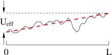
Figure 2: A typical realization of the potential in the continuum limit of the Sinai model (smooth curve) and the potential in the corresponding effective medium (dashed).

To perform this transformation, we use Eq. (2) to solve for $v$ as a function of $E_{+}$ for fixed $f$. This inversion is feasible only for $f=\frac{1}{2},\frac{1}{3},\frac{1}{4},\frac{1}{5}$, because solving a polynomial up to quartic order is involved. For the simplest case of a particle starting at the midpoint, $f=\frac{1}{2}$, then (2) becomes $E_{+}=1/(1+z)$. Inverting gives

$$v(E_{+})=\frac{2D}{L}\ln\frac{E_{+}}{E_{-}}\qquad\frac{dv}{dE_{+}}=\frac{2D}{LE_{+}E_{-}}~{}.$$ (5)

Substituting these results into Eq. (3) and using (4) gives,

$$\mathcal{P}(E_{+})\!=\!\frac{1}{\sqrt{2\pi\sigma_{v}^{2}}}\frac{2D}{LE_{+}E_{-}}\exp\left[-\frac{2D^{2}}{\sigma_{v}^{2}L^{2}}\ln^{2}\!\left(\frac{E_{+}}{E_{-}}\right)\right]\!.$$ (6)

We now relate the velocity variance $\sigma_{v}^{2}$ to the disorder in the Sinai model. For Sinai disorder, the mean-square potential difference between two points separated by a distance $L$ is (Fig. 2)

$$U_{\rm eff}^{2}\equiv\int_{0}^{L}\int_{0}^{L}\ \langle F(x^{\prime})F(x^{\prime\prime})\,\rangle dx^{\prime}dx^{\prime\prime}=\sigma^{2}_{F}\,L\,.$$

Thus there is a net force $F_{\rm eff}\sim U_{\rm eff}/L\sim\sigma_{F}/\sqrt{L}$, from which we infer the velocity scale $\sigma_{v}\sim\sigma_{F}/(\gamma\sqrt{L})$, where $\gamma$ is the viscosity coefficient. We then use the fluctuation-dissipation relation $D=kT/\gamma$ to rewrite Eq. (6) as

$$\mathcal{P}(E_{+})\!=\!\frac{1}{\sqrt{4\pi\alpha}}\frac{1}{E_{+}E_{-}}\exp\left[-\frac{1}{4\alpha}\ln^{2}\!\left(\!\frac{E_{+}}{E_{-}}\!\right)\right]\!,$$ (7)

with $\alpha=\sigma_{F}^{2}\,L/[8(kT)^{2}]$ a dimensionless measure of the strength of the Sinai potential relative to thermal fluctuations. The important feature of this splitting probability distribution is its change from unimodal to bimodal as the disorder parameter $\alpha$ increases past $\alpha_{c}=1$ (Fig. 3).

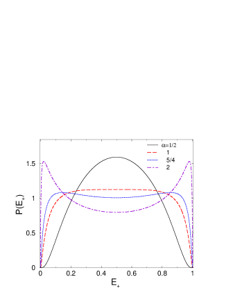
Figure 3: (color online) Optimal fluctuation prediction for the splitting probability distribution for the Sinai chain when the particle starts at $Y=L/2$ (top) and $Y=L/3$ (bottom, logarithmic scale).

In the critical case $\alpha=\alpha_{c}$ the maximum at $E_{+}=1/2$ is quartic and the distribution is close to uniform for $0.2\lesssim E_{+}\lesssim 0.8$. Thus any value of $E_{+}$ in this range is nearly equally probable. For $\alpha\gtrsim\alpha_{c}$, two maxima emerge continuously at $E_{+}=\frac{1}{2}[1\pm\sqrt{3(\alpha-\alpha_{c})}]$. Curiously, although the disorder-average value $\langle E_{+}\rangle=1/2$, for $\alpha>\alpha_{c}$ the probability distribution has a minimum at $E_{+}=1/2$. In this strong disorder limit, the underlying mechanism for the bimodality of the distribution is that a typical realization of the environment has a net bias (see Fig. 2) so that the splitting probability is either close to zero or to one.

For $f=\frac{1}{3}$, a similar calculation gives the splitting probability distribution shown in Fig. 3. For weak disorder, the splitting probability is peaked at a point close to the value $\frac{1}{3}$ that arises in the case of no disorder. When $\alpha$ is sufficiently large, the splitting probability has peaks near 0 and 1, corresponding to strong disorder where a typical configuration has an overall net bias. The intermediate regime of $\alpha$ gives the strange situation in which there is a peak at one extremum but not the other.

For a general starting point, the inversion $v=v(E_{+})$ and thus the form of $\mathcal{P}(E_{+})$ can be determined asymptotically in the limits $|vL/D|\to\infty$. For $vL/D\to-\infty$, $z\to+\infty$, and Eq. (2) becomes $E_{+}\sim z^{-(1-f)/f}$. Solving for $v(E_{+})$ and $\frac{dv}{dE_{+}}$ and using these results in Eq. (4), the splitting probability distribution starting from $Y=fL$ is

$$\mathcal{P}(E_{+})=\frac{1}{\sqrt{16\pi\alpha}}\frac{1}{(1\!-\!f)E_{+}}\,\exp\left[-\frac{\ln^{2}E_{+}}{16\alpha(1\!-\!f)^{2}}\right].$$ (8)

As $\alpha$ is varied, this distribution changes from having a peak at the most probable value of $E_{+}$ to a peak at $E_{+}=0$. In the complementary limit $vL/D\to+\infty$, corresponding to $z\to 0$ and $E_{+}\to 1$, the distribution is again (8), but with $f\to 1-f$ and $E_{+}\to 1-E_{+}$.

We now give an exact solution for the splitting probabilities that qualitatively substantiates the heuristic results given above. Consider the Fokker-Planck for the probability distribution for a particle that moves in the Sinai potential, $P_{t}=D\left[P_{xx}-\beta(F(x)P)_{x}\right]$, where $\beta=1/kT$ and $P(x,t)\,dx$ is the probability that the particle is in the range $[x,x+dx]$ at time $t$ and $F(x)$ is the force at $x$. Suppose that particles are injected at a constant rate at $Y$ to maintain a fixed concentration $P(Y)=1$ when absorbing boundary conditions at $x=0$ and $x=L$ are imposed. Then the stationary solution to the Fokker-Planck equation is

$$P(x)=\begin{cases}e^{\beta\mathcal{F}_{Y}(x)}\left[1-{\displaystyle\frac{\int_{Y}^{x}\exp[-\beta\mathcal{F}_{Y}(x)]\,dx}{\int_{Y}^{L}\exp[-\beta\mathcal{F}_{Y}(x)]\,dx}}\right]&x\geq Y\\ \\ e^{\beta\mathcal{F}_{Y}(x)}\left[1-{\displaystyle\frac{\int^{x}_{Y}\exp[-\beta\mathcal{F}_{Y}(x)]dx}{\int^{0}_{Y}\exp[-\beta\mathcal{F}_{Y}(x)]\,dx}}\right]&x\leq Y,\end{cases}$$ (9)

where $\mathcal{F}_{Y}(x)\equiv\int^{x}_{Y}dx^{\prime}F(x^{\prime})$.

From the steady current $J=-D[P_{x}-\beta(F(x)P)]$, the splitting probabilities $E_{\pm}(Y)$ are simply

$$E_{-}=\frac{\tau_{+}}{\tau_{-}+\tau_{+}}~{},\qquad E_{+}=\frac{\tau_{-}}{\tau_{-}+\tau_{+}}$$ (10)

where $\tau_{\pm}=1/J_{\pm}$, with $J_{\pm}$ being the flux to the boundaries at 0 and $L$, respectively. Thus $\tau_{\pm}$ define the “resistance” of a finite interval with respect to passage across the two boundaries and are given explicitly by

$$\tau_{-}=\int_{0}^{Y}e^{-\beta\mathcal{F}_{0}(x)}\,dx,\quad\tau_{+}=\int_{0}^{L-Y}e^{-\beta\mathcal{F}_{0}(x)}\,dx.$$ (11)

We emphasize that the force integrals $\mathcal{F}_{0}$ are independent variables in each integrand so that $\tau_{-}$ and $\tau_{+}$ are also independent random variables.

The quantities defined in (11) are the continuous-space counterparts of Kesten variables kesten that play an important role in many stochastic processes. For example, negative moments of $\tau$ describe the positive moments of a steady diffusive current in a finite Sinai chain bur1 ; osh1 ; osh2 ; comtet1 ; comtet2 . A surprising feature is that the disorder-average currents $J_{\pm}$ scale with system length $L$ as $L^{-1/2}$ and are much larger than Fickian which scale as $L^{-1}$ in homogeneous environments. Thus Sinai chains have an anomalously high conductance despite the fact that diffusion is logarithmically confined sinai and positive moments of $\tau$ grow as $e^{\sqrt{L}}$ bur1 ; osh1 ; osh2 ; comtet1 ; comtet2 .

Let $\Psi_{-}(\tau_{-})$ and $\Psi_{+}(\tau_{+})$ denote the distribution functions of the random variables $\tau_{-}$ and $\tau_{+}$, respectively. Then the moment generating function of the splitting probability $E_{+}$ can be written as:

$$\langle e^{-\lambda E_{+}}\rangle\!=\!\int_{0}^{\infty}\!\!\!\!\int_{0}^{\infty}\!\!\!\Psi_{-}(\tau_{-})\Psi_{+}(\tau_{+})\,e^{-\lambda\tau_{-}/(\tau_{-}+\tau_{+})}\,d\tau_{-}d\tau_{+}.$$ (12)

Integrating over $d\tau_{+}$, we formally change the integration variable from $\tau_{+}$ to $E_{+}$ to give

$$\langle e^{-\lambda E_{+}}\rangle=\int^{1}_{0}\frac{dE_{+}}{E_{+}^{2}}e^{-\lambda E_{+}}\!\!\!\int^{\infty}_{0}\!\!\!\!d\tau_{-}\,\tau_{-}\Psi_{-}(\tau_{-})\Psi_{+}(r\tau_{-}),$$

where $r=E_{-}/E_{+}$. From this expression we may read off the following form of the probability density $\mathcal{P}(E_{+})$ of the splitting probability $E_{+}$:

$$\mathcal{P}(E_{+})=\frac{1}{E_{+}^{2}}\int^{\infty}_{0}d\tau_{-}\,\tau_{-}\Psi_{-}(\tau_{-})\Psi_{+}(r\tau_{-}).$$ (13)

For a random potential without any bias, the distribution $\Psi_{-}(\tau_{-})$ is given by (see, e.g., Ref. comtet2 ):

$$\Psi_{-}(\tau_{-})\!\! = \!\!\frac{\sqrt{fL}}{2\pi\alpha_{-}\tau_{-}^{3/2}}\int_{-\infty}^{\infty}\!\!\!du\,{\rm ch}\,u\,\cos\left(\frac{\pi u}{2\alpha_{-}}\right)$$ (14)

$$\times \exp\left[\frac{\pi^{2}}{8\alpha_{-}}-\frac{u^{2}}{2\alpha_{-}}-\frac{2fL\,\,{\rm ch}^{2}u}{4\alpha_{-}\tau_{-}}\right],$$

where $\alpha_{-}=\beta^{2}\sigma_{F}^{2}fL/4$ and ${\rm ch}\,u$ denotes the hyperbolic cosine. Then $\Psi_{+}(\tau_{+})$ is obtained from (14) by replacing $\tau_{-}\to\tau_{+}$ and $\alpha_{-}\to\alpha_{+}=\beta^{2}\sigma_{F}^{2}(1-f)L/4$.

Substituting $\Psi_{-}(\tau_{-})$ and $\Psi_{+}(\tau_{+})$ into Eq. (13) and integrating over $d\tau_{-}$, we find

$$\mathcal{P}(E_{+}) = \frac{1}{\pi^{2}\sqrt{4\alpha_{-}\alpha_{+}E_{+}E_{-}}}\int_{-\infty}^{\infty}\!\int_{-\infty}^{\infty}du_{1}\,du_{2}$$ (15)

$$\times \frac{\,{\rm ch}\,u_{1}\,{\rm ch}\,u_{2}}{E_{-}{\rm ch}^{2}u_{1}+E_{+}{\rm ch}^{2}u_{2}}\cos\left(\frac{\pi u_{1}}{2\alpha_{-}}\right)\cos\left(\frac{\pi u_{2}}{2\alpha_{+}}\right)$$

$$\times \exp\left[\frac{\pi^{2}}{8\alpha_{-}}+\frac{\pi^{2}}{8\alpha_{+}}-\frac{u_{1}^{2}}{2\alpha_{-}}-\frac{u_{2}^{2}}{2\alpha_{+}}\right].$$

After cumbersome but straightforward manipulations, one of the integrals can be performed to recast the splitting probability distribution as:

$$\mathcal{P}(E_{+}) =\frac{1}{\pi\sqrt{4\alpha_{-}\alpha_{+}E_{+}E_{-}}}\frac{1}{E_{-}}\int_{-\infty}^{\infty}du\,\frac{{\rm ch}\,u}{{\rm ch}\,\eta}\cos\left(\frac{\pi u}{2\alpha_{+}}\right)$$ (16)

$$\times \exp\left[\frac{\pi^{2}}{8\alpha_{+}}-\frac{u^{2}}{2\alpha_{+}}-\frac{\eta^{2}}{2\alpha_{-}}\right],$$

where $\eta={\rm sh}^{-1}\left[({\rm ch}\,u)/\sqrt{r}\right]$. For the symmetric initial starting point, $\alpha_{+}=\alpha_{-}=\alpha$, the distribution changes from unimodal to bimodal as $\alpha$ increases beyond $\alpha_{c}\approx 0.815$ (Fig. 4).

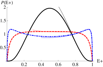
Figure 4: (color online) Exact distribution $\mathcal{P}(E_{+})$, Eq. (16). for $\alpha_{-}=\alpha_{+}=1/4$ (solid curve) $\alpha_{\pm}=0.815$ (dashed), and $\alpha_{\pm}=1.2$ (dash-dotted). Thin curves are the corresponding asymptotic results of Eq. (17).

To extract the asymptotic behavior of $\mathcal{P}(E_{+})$ in the limits $E_{+}\to 1$ and $E_{+}\to 0$ note that because the integrand in Eq. (16) contains an oscillating cosine term, only the behavior near $u=0$ should matter. Thus assuming ${\rm ch}\,u\approx 1$ and expanding $\eta^{2}$ in a Taylor series in $u$ up to second order, we find the following asymptotic representation for $E_{+}\to 1$:

$$\mathcal{P}(E_{+}) \sim\frac{\left(\alpha_{-}+\alpha_{+}\sqrt{E_{+}}\ln z_{+}\right)^{-1/2}}{\sqrt{2\pi E_{+}}\,\,E_{-}}$$ (17)

$$\times \!\!\!\!\!\!\!\!\!\exp\!\left[-\frac{\ln^{2}z_{+}}{2\alpha_{-}}\!+\!\frac{\pi^{2}\sqrt{E_{+}}\ln z_{+}}{8\left(\alpha_{-}+\alpha_{+}\sqrt{E_{+}}\ln z_{+}\right)}\right]\!,$$

where $z_{+}=(1+\sqrt{E_{+}})/\sqrt{E_{-}}$. This asymptotic form agrees quite well with the exact result in Eq. (16), not only when $E_{+}\to 1$, but also for moderate values of $E_{+}$ (Fig. 4). Similarly, we obtain the asymptotics of $\mathcal{P}(E_{+})$ for $E_{+}\to 0$ merely by interchanging all subscripts $\pm$ to $\mp$ in (17), and $z_{-}$ is obtained from $z_{+}$ by interchanging the subscripts $\pm$ to $\mp$ in the latter. When $E_{+}\ll 1$ or $1-E_{+}\ll 1$ respectively, Eq. (17) reduces to

$$\mathcal{P}(E_{+})\sim\sqrt{\frac{1}{\pi\alpha_{\pm}\ln\left(1/E_{\mp}\right)}}\frac{1}{E_{\mp}}e^{-\frac{1}{8\alpha_{\mp}}\ln^{2}\left(\frac{1}{E_{\mp}}\right)}~{}.$$ (18)

Our optimal fluctuation result (7) resembles the above form apart from logarithmic and numerical factors.

In summary, by making an analogy to first passage on a Sinai chain, we find that the evolution of a partially melted random heteropolymer at the melting temperature is controlled by the sequencing of monomers. Each heteropolymer realization has a unique kinetics and final fate that is not representative of the average behavior of an ensemble of such polymers. A related lack of self averaging was recently found in anomalous diffusion LSK .

Acknowledgments. We gratefully acknowledge helpful discussions with O. Bénichou. GO is partially supported by Agence Nationale de la Recherche (ANR) under grant “DYOPTRI - Dynamique et Optimisation des Processus de Transport Intermittents” while SR is partially supported by NSF grant DMR0535503 and the University of Paris VI.

References

(1) R. M. Wartell and E. W. Montroll, Adv. Chem. Phys. 22,
129 (1972).
(2) D. Poland and H. R. Scheraga, Theory of Helix Coil
Transition in Biopolymers (Academic, New York, 1970).
(3) M. Ya. Azbel, Phys. Rev. A 20, 1671 (1979).
(4) H. A. Scheraga, J. A. Vila and D. R. Ripoll,
Biophys. Chem. 101-102, 255 (2002)
(5) P. G. de Gennes, J. Stat. Phys. 12, 463 (1975).
(6) Ya. G. Sinai, Theor. Probab. Appl. 27, 256 (1982).
(7) S. Redner, A Guide to First-Passage Processes, (Cambridge
University Press, New York, 2001).
(8) I. M. Lifshitz, S. A. Gredescul, and L. A. Pastur, An
Introduction to the theory of disordered systems (Wiley, New York,
1988).
(9) H. Kesten, Acta Math. 131, 207 (1973)
(10) S. F. Burlatsky, G. Oshanin, M. Mogutov and M. Moreau, Phys. Rev. A 45, 6955 (1992)
(11) G. Oshanin, M. Mogutov and M. Moreau, J. Stat. Phys. 73, 379 (1993)
(12) G. Oshanin, S. F. Burlatsky, M. Moreau and B. Gaveau, Chem. Phys. 177, 803 (1993)
(13) C. Monthus and A. Comtet, J. Phys. I France 4, 635 (1994)
(14) C. Monthus, A. Comtet and M. Yor, J. Appl. Prob. 35, 255 (1998)
(15) A. Lubelski, I. M. Sokolov, and J. Klafter, Phys. Rev. Lett. 100 250602 (2008).