Stochastic resonance and the trade arrival rate of stocks

Abstract

We studied non-dynamical stochastic resonance for the number of trades in the stock market. The trade arrival rate presents a deterministic pattern that can be modeled by a cosine function perturbed by noise. Due to the nonlinear relationship between the rate and the observed number of trades, the noise can either enhance or suppress the detection of the deterministic pattern. By finding the parameters of our model with intra-day data, we describe the trading environment and illustrate the presence of SR in the trade arrival rate of stocks in the U.S. market.

1 Introduction

It can be very useful to model and understand market microstructure. For instance, it has been shown that the number of trades and volume can help explain volatility fluctuations and therefore help model asset returns [2, 10, 28]. More importantly, these studies link market activity (and therefore market microstructure) to the large class of asset allocation and pricing models based on time changed Brownian motion [9, 23, 27]. More practically, we also point to the increase of intra-day trading that some claim should account for more than $50\%$ of the trading volume by 2010. High-frequency trading will increasingly require market microstructure for risk control and trading.

In this paper, we use the doubly stochastic Poisson process to model the number of trades inside of a trading day. Using this model, we focus on the interaction between noise and the trade rate ”U”-shaped pattern (higher average arrival rate at the open and close of the trading day). We report an interesting feature of such model: stochastic resonance (SR). The presence of stochastic resonance indicates that a correct amount of noise is, in fact, beneficial to increase the detection of the ”U”-shaped pattern. That is, random trading (represented by random arrival rates) can constructively contribute to the existence of such periodic patterns.

1.1 ”U”-shaped pattern

Finance and economics show a variety of well documented periodic patterns [14]. In particular, there is the intra-day ”U”-shaped pattern (or patterns). That is, the average intra-day volatility, the trading volume, bid-ask spreads, trading activity (number of trades), and even returns are significantly higher near the open and close of the trading day [7, 20, 21, 24, 30]. These quantities form on average an ”U” shape; hence, the name ”’U’-shaped pattern”. In fact, it has been shown that there need not be a official exchange halt. Studies using 24-hour markets (such as currency markets) find that ”U”-shaped patterns are also present within the normal business hours [11].

There is a large literature that explains the different ”U”-shaped patterns. In general the literature has been grouped into two lines: The first line suggests that asymmetric information is a necessary condition for the ”U” shape to exist. By asymmetric information, it is meant that some traders have private information about the future asset returns [1] or payoffs [18]. It is the interplay between informed traders and uniformed traders together with market stops that will lead to the observed pattern both in returns and volumes [18].

The second line contests the importance of asymmetric information by pointing out to the presence of the same patterns in markets with no asymmetric information [11, 12]. They argue that the presence of market stops could be enough. This line emphasizes the exchange of risk close to market stops [16]. The argument is that information accumulated overnight will generate an increase of the trading activity at market open because portfolio managers will want to bring their portfolio to a particular risk target as soon as possible. The same will happen at the end of a trading day, when traders will want to prepare themselves for the next overnight period. Therefore, the pattern could be just due to the timing of transaction decisions by institutional investors and long-term investors with short term investors representing the other side of the trade [6].

In this paper we do not address the micro-economical origin of such patterns as, for instance, in Hong and Wang [18]. We take an empirical approach to the problem. We start with a plausible statistical model which describes the data well. Since our model presents stochastic resonance, we conjecture that such a phenomenon can be important to the ”U” pattern. The presence of SR could indicate that noise traders can, in fact, magnify such pattern. However, in the present paper we will not be able to reach such level of description, leaving such questions for future studies.

From a practical point of view, our work still presents useful results. For instance, one can also think on a possible algorithm where random trading (hence undetected to other traders) can enhance even further such a pattern. Of course, the benefit of enhancing such a pattern is, a priori, not clear. But in a similar fashion there could be other patterns where similar analysis will lead to undetected (and beneficial to the trader) market manipulation. We also point to the analogy drawn recently by Dempster et al. [13] as a possible starting point to generalize SR to asset allocation, for instance.

1.2 Stochastic resonance

Stochastic resonance (SR) has been successfully used to explain signal transmission and detection in a wide variety of systems in diverse areas such as physics, geology, neural science, engineering, and biology [15]. SR is briefly defined as noise-enhanced signal detection. Typically there is a threshold below which the signal cannot be detected. Adding noise to the signal can increase the number of events that cross such a threshold, hence increasing the detection of such signal. Imagine a sine wave of amplitude less than the detection barrier. Noise added to the sine wave will increase the events that cross the detection barrier. However, if the noise intensity is too high, it will corrupt the signal beyond recognition.

In finance, stochastic resonance has been suggested to explain market crash and high-frequency patterns in the exchange rate [19, 25]. Different from previous work, our paper employs non-dynamical, threshold-free stochastic resonance [4, 5]. Non-dynamical SR is purely stochastic in nature and, therefore, it does not require a microscopic model (such as Newton’s equations of motion). Consequently, it can be more general because it dissociates a specific microscopic model from the SR phenomenon. To the best of our knowledge, this is the first time this particular SR class has been applied to financial data.

2 Non-dynamical stochastic resonance

In direct analogy to non-dynamical SR in other disciplines, we assume that trade arrivals follow a time-dependent Poisson process. We take the point of view of a market participant and observer. We observe signals in the market that are being transmitted to all market participants. Our goal is to describe the present state of the trading environment and therefore detect the presence of SR.

Non-dynamical and threshold-free stochastic resonance was originally discovered for systems that can be modeled with a doubly stochastic Poisson process (or time-dependent Poisson process) [5]. Such a process is constructed out of Poisson process $N(t)$ with the probability distribution of $n$ events during time interval $T$ given by

$$p_{N}(n)=\frac{e^{-rT}(rT)^{n}}{n!},$$ (1)

where the event arrival rate $r$ is itself a time dependent random process independent of $N(t)$ [3]. Bezrukov and Vodyanoy have shown that the following arrival rate $r(t)$ of a doubly stochastic Poisson process exhibits SR:

$$r(t)=r(0)\exp(A(t)),$$ (2)

with $A(t)$ as

$$A(t)=W(t)+A_{s}\cos(2\pi f_{s}t).$$ (3)

That is, $A(t)$ is the sum of zero mean Gaussian noise $W(t)$ with root mean square $\sigma$; and a weak periodic signal with amplitude $A_{s}$ and frequency $f_{s}$ [5].

In the case of Equation (3), the slow cosine-wave $A_{s}\cos(2\pi f_{s}t)$ can be better detected, due to SR, by analyzing the final Poisson generated time series $N(t)$ if there is a correctly tuned noise $W(t)$. However, excessive noise might corrupt the signal.

2.1 Signal-to-noise ratio

For a quantitative analysis of the synchronized process, signal-to-noise ratio (SNR) is introduced to measure stochastic resonance. SNR is defined as the height of the signal divided by the height of the noise background of the power spectrum at the signal frequency $f_{s}$ [15]. We speak of SR if there is a maximum in the output SNR as a function of noise intensity $\sigma$. That is, there is an optimal value of the noise that concurs with the periodic signal.

Bezrukov and Vodyanoy derived the output SNR for the doubly stochastic Poisson process with the rate given by Equation (2) and Equation (3) via power spectral density for $A_{s}\ll\sigma$ and $f_{s}$ much smaller than all other characteristic frequencies. The output SNR is given by

$$SNR=\frac{(A_{s}^{2}r(0)/2)\exp(\sigma^{2}/2)}{2+(2r(0)/\pi f_{c})\exp(\sigma^{2}/2)\sum_{n=1}^{\infty}(1/n)(\sigma^{2n}/n!)},$$ (4)

where $f_{c}$ is the noise corner frequency [4, 5]. We also have $f_{c}=(2\pi\tau_{c})^{-1}$, where $\tau_{c}$ is the noise $W(t)$ correlation time. The noise has a Lorentzian power spectrum with exponential autocorrelation function. We have also verified Equation (4) by Monte Carlo (MC) simulating Equation (1) with rate given by Equations (2) and (3) [8]. Using our MC simulations, we remark that Equation (4) is still a very good approximation outside the range of parameters for which it has been derived [5].

The maximum SNR as a function of $\sigma$ in Equation (4) is the result of a competition between the exponential in the numerator and the exponential times a linear term (to first order approximation) in the denominator. The constant $A_{s}^{2}r(0)/2$ is a general scale of the amplitude of the maximum. The location of the maximum is given by $r(0)/f_{c}$. $r(0)/f_{c}$ is the number of events that occur over the correlation time. If $r(0)/f_{c}$ is large, the maximum moves to small $\sigma$; if $r(0)/f_{c}$ is small the maximum moves to large $\sigma$. Therefore, the existence of the maximum depends entirely on $r(0)/f_{c}$: SR is more important for a random variable where the statistics is poor; that is, the equilibrium arrival rate $r(0)$ is small. SR is also more important when the noise present (or added) to the system is uncorrelated. Furthermore, it also shows that no matter how good $r(0)$ is, the output signal detection could be further improved if $f_{c}$ is big enough. Equation (4) shows that if the condition $f_{c}>2r(0)\pi$ [$\tau_{c}r(0)<0.25$] holds, the process demonstrates SR.

3 Numerical experiments

We cannot always perform controlled experiments in economics; therefore, we need to extract all the needed information from the data we observe. We first parameterize the time dependent rate $r(t)$ defined by Equations (2) and (3) without the Gaussian noise $W(t)$ by assuming that parameters for the rate are constant for at least $1$ month. We have

$$r(t)=r(0)e^{A_{s}\cos(2\pi f_{s}t)},$$ (5)

where $f_{s}$ is one over the trading day, $f_{s}=1/23400$ seconds. Notice that once we have detected the periodic signal $A_{s}\cos(2\pi f_{s}t)$, we have bypassed one of the potential benefits of SR: increasing statistics to help the signal detection. Therefore, we cannot infer if our signal reconstruction was helped by SR. However, we can still say that a system can potentially present SR by identifying all the parameters.

In our numerical experiments, we obtained tick-by-tick financial data (smallest time resolution is $1$ second) for $12$ trading stocks (AA,AEP, AES, AMG, AOL, ATI, EK, F, JPM, PFE, PG, and S) during $21$ trading days (January 2001). First, we analyze the daily pattern by constructing a proxy for the trade arrival rate inside of the $6.5$ hours composing the trading day. We bin the data in $2$-minute ($120$-second) intervals using $1$-second resolution from the first day to the last day (total of $21$ days). We assume that the rate in each of the $2$-minute bin is constant. We remove the first $5$ minutes at the beginning of the trading day due to data inaccuracy. We end up with a total of 192 $2$-minute intervals in a day.

We then calculate the arrival rate for every $2$ minutes by counting the number of trades in every interval and dividing by $120$ seconds; that is, the average number of trades in each of the $192$ bins during $21$ days. This is equivalent to fitting a constant rate Poisson process since the maximum likelihood estimate for the rate is simply the average number of events per unit of time. Once we have the empirical daily rate pattern, we fit the daily rate pattern to Equation (5) to estimate $r(0)$ and $A_{s}$.

FIG. 1 shows the arrival rate averaged over $21$ days and all $12$ stocks. In order to average over all stocks, we subtract $\ln(r(0))$ from the natural logarithm of the empirical rate of each stock and then multiple by $1/A_{s}$ to obtain $\cos(2\pi f_{s}t)$. Thus, we are able to recover the parameter independent $\exp(\cos(2\pi f_{s}t))$. Equation (5) is a very simple periodic function and hence the most simple example one can choose. However, FIG. 1 shows that it gives a good approximation to the empirical daily rate pattern especially for the second half of the day. The first half is on average systematically higher indicating that a skewed function could be better. Nonetheless, since $r(0)$ measures the vertical shift of the whole curve, the value of $r(0)$ will not change very much even if asymmetry is taken into account. The quality of our approximation will suffice for defining SR.

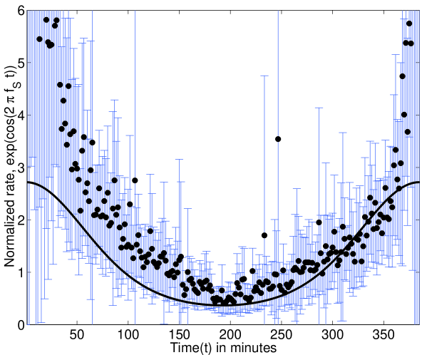
Figure 1: Normalized average intra-day arrival rate pattern for 12 stocks. The number of trades per unit of time (2-minute bins are used here) are chosen as a good proxy for the arrival rate of trades. The symbols are the average over 21 days and 12 stocks. The error bars represent 1 standard deviation of the empirical data. The solid line is the theoretical model in Equation (5).

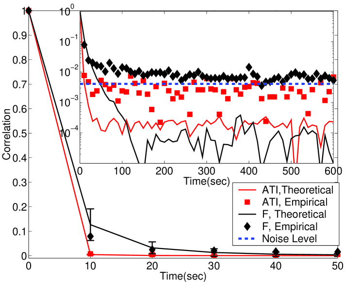
Figure 2: Autocorrelation of the number of trades for $2$ stocks (ATI and F). The symbols represent the empirical autocorrelation for the data, and the solid lines represent the theoretical autocorrelation constructed via MC simulation. The inset presents the behavior of the tails in log-linear scale.

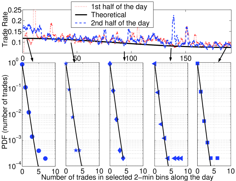
Figure 3: The top panel of the graph shows the daily trading rate pattern [Eq. (5)] for F. The bottom graphs are the selected PDFs of 2-minute intervals along the trading day for F; the symbols are data points, and the lines are the theoretical PDF. Once the daily pattern is found (top panel), we fit all 2-minute empirical PDFs along the day with one single parameter $\sigma$ (lower panel).

After $r(0)$ and $A_{s}$ have been estimated, the remaining fluctuation are assumed to be generated from the random process $W(t)$ with intensity $\sigma$ [Eq. (3)]. At this stage, we only need to find $\tau_{c}$ (or $f_{c}$) [Eq. (4)] to demonstrate the presence of SR for a given stock.

We find $\tau_{c}$ indirectly through the autocorrelation function of the number of trades $N(t)$. Notice that $\tau_{c}$ measures the characteristic memory of the Gaussian noise $W(t)$ in Equation (3). However, we cannot measure the autocorrelation of $W(t)$ since $W(t)$ cannot be observed from the data directly. Furthermore, we can achieve a 1-second resolution by using the autocorrelation $N(t)$, since $N(t)$ is directly observed from the market.

We find the autocorrelation of the number of trades for our model by Monte Carlo (MC) simulating Equations (1), (2), and (3). We simulate a time series of the number of trades $N(t)$ with a band-limited white noise $W(t)$ of corner frequency $f_{c}$. For every $f_{c}$ (or $\tau_{c}$) there will be a time series of the number of trades. For every such time series, we have an autocorrelation function. The correlation time $\tau_{c}$ for a given stock is the one which minimizes the mean square error between the simulated autocorrelation and the empirical autocorrelation function.

FIG. 2 presents the autocorrelation of the number of trades $N(t)$ for two stocks, ATI and F. We calculate the autocorrelation function using all $21$ days of tick-by-tick data (a total of $\approx 530000$ data points). These stocks represent the typical autocorrelation for our $12$ stocks. We are able to model autocorrelation function up to correlations of the order of $1\%$. However, in agreement with the literature, some stocks clearly present a slow decaying autocorrelation. Notice that F has a slow decaying tail above the autocorrelation noise level ($\approx 3/\sqrt{(}530000)=0.0041$). ATI, however, decays faster and has no significant autocorrelation.

The presence of a persistent tail for F shows that the autocorrelation could better modeled either by 2 exponentials (two different $\tau_{c}$) or by a power law. The exponential autocorrelation function with a single $\tau_{c}$ is, therefore, a first order approximation. However, such first order approximation will suffice to define SR. We note that is highly unlikely that $\tau_{c}$ will be small enough for a stock to present a maximum in SNR and still have a large and significant autocorrelation tail. That is, most of the autocorrelation ($>99\%$) is generally explained by a single exponential function. If a stock has a large autocorrelation tail, it will have a large $\tau_{c}$ as happens with F (and not with ATI).

The noise intensity $\sigma$ defines the present trading environment in the SNR graph [FIG. (4)]. We find $\sigma$ by fitting the theoretical probability density function (PDF) of the doubly stochastic Poisson process to the empirical PDF [26]. Note that $r(0)$ and $A_{s}$ were estimated previously via Equation (5). We replace the previously estimated $r(0)$ and $A_{s}$ into Equation (2). We continue with the approximation that every 2-minute interval is described by doubly stochastic Poisson process with constant arrival rate $r(0)\exp(A_{s}\cos(2\pi f_{s}t))$ perturbed by noise. Thus, within each 2-minute interval, the noise can be described by the log-normal distribution $\exp(W(t))$. We apply numerical integration to calculate the integral of the log-normal (which defines the random rate) and the Poisson (which takes this random rate) to find the PDF of number of arrivals in every 2-minute interval. Since the number of arrivals in 2-minute intervals are small, we compensate the small number of arrivals by fitting all the 2-minute intervals in a trading day at once to obtain $\sigma$ by the mean square method.

FIG. 3 shows the daily trading pattern by binning a trading day into $2$-minute intervals for F (other stocks present similar results). The top part of the figure is the daily trading pattern. For a cosine function, the first half of the day is the mirror image of the second half. We put both halves on top of each other. The solid thick line is obtained from our model. After finding the parameterized mean, all the data points are fitted at once to estimate the noise volatility $\sigma$. The bottom part of the figure shows selected PDFs for few 2-min intervals along the trading day. For instance, the first PDF represents the first and the last 2-minute intervals of the trading day. FIG. 3 shows that our simple model with a single $\sigma$ can fit the empirical PDF up to $4$ orders of magnitude. This remarkable agreement is found for all stocks studied along the entire trading day.

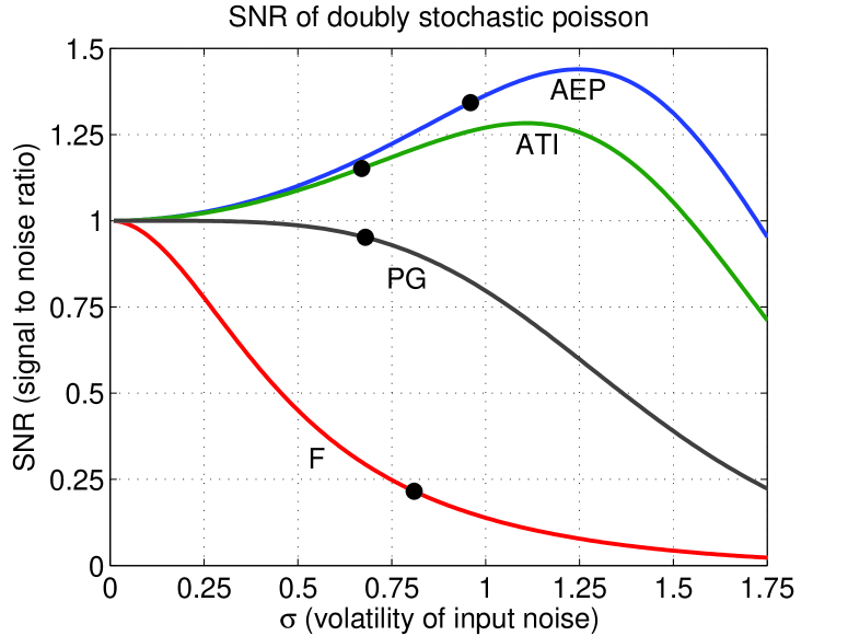
Figure 4: Output signal to noise ratio (SNR) of 4 trading stocks (AEP, ATI, PG, F) using Eq. (4). The circles are the current value of $\sigma$. The figure shows that SR occurs at different levels in AEP and AIT, but not in F and PG.

Once $\sigma$ is obtained by our scheme, we have described the trading environment using our model; thus, stocks that present SR can be identified. FIG. 4 shows the SNR as a function of noise intensity. We have normalized all SNR curves such that the SNR for $\sigma=0$ is equal to $1$ for all stocks. Table 1 has the recovered values for the parameters of our model. We can see that, in fact, stocks that satisfy $r(0)\tau_{c}<0.25$ such as AEP and ATI present a maximum on the SNR (and, hence, show SR). From our sample of $12$ stocks, $1/2$ show SR. The largest $r(0)$ for the stocks that present SR is $\approx 4$ trades per minute, whereas, theoretically, we need to have $r(0)<15$ per minute (assuming that $\tau_{c}=1$ sec is the lowest possible value). These results indicate that the less-traded stocks are more likely to present SR. Usually the less-traded stocks are stocks with smaller market capitalization. Therefore, SR should be more important for small cap stocks.

	$r(0)(1/sec)$	$A_{s}$	$\sigma$	$\tau_{c}(sec)$	$\tau_{c}r(0)$
AEP	0.0283	0.2880	0.9554	1.7000	0.05
ATI	0.0146	0.1253	0.6688	4.7000	0.05
PG	0.0946	0.2856	0.6839	2.6000	0.26
F	0.0947	0.2194	0.8118	26.5000	2.60

Table 1: Parameter values for FIG. 4.

The values in Table 1 together with FIG. 4 describe the statistical trading environment. From the point of view of a market observer, the signal of interest ($A_{S}\cos(2\pi f_{c}t)$) is being transmitted more efficiently (ATI and AEP) or less efficiently (F and PG) with the help of noise present in the trading environment. From a point of view of a market participant, both AEP and ATI are not at the SNR maximum. Therefore, adding noise by adding trades with a random arrival rate should increase the detection of the arrival rate ”U”-shaped pattern. In the case of AEP, for instance, a $25\%$ increase in the noise intensity is beneficial to the periodic pattern.

4 Conclusion

We have proposed to model the number of stock trades inside of the trading day with a doubly stochastic Poisson process. With a doubly stochastic Poisson process, we are able to model both the deterministic periodic trend (”U”-shaped pattern) in the trade arrival rate as well as deviations from it due to noise. We show that such model describes well the empirical data and that non-dynamical stochastic resonance can be a relevant phenomena for the ”U”-shaped pattern detection. SR as presented in this paper is defined as a weak regular oscillation that may be amplified by adding noise to the input signal. That means that the increase of noise trading (represented here with an increase in the random trade rate) can, in fact, augment the relevance of the exiting ”U”-shaped pattern.

We envision that extensions of the model presented in this work could be possible for different economical time series. In our theoretical framework, the presence of a periodic pattern is a necessary condition for SR to be relevant. We know that such periodic patterns are, in fact, present in economics in general (see [14, 17, 22, 29] for additional examples), therefore making SR a potentially important phenomena.

Acknowledgments. We are grateful to Peter Carr and Lee Deville for enlightening discussions. We thank Samir Garzon for suggestions to improve our work as well as detailed discussions. We thank Sergey Bezrukov for pointing us to useful references, and Robert H. Smith School of Business at UMCP for providing tick-by-tick data. We thank also Professor Jonathan Goodman of the Courant Institute of Mathematical Sciences at New York University for his encouragement and support.

References

- [1] Anat R. Admati and Paul Pfleiderer. Divide and conquer: A theory of intraday and day-of-the-week mean effects. The Review of Financial Studies, 2(2):189–223, 1989.
- [2] Thierry Ané and Hélyette Geman. Order flow, transaction clock, and normality of asset returns. The Journal of Finance, 55(5):2259–2284, 2000.
- [3] Vladimir E. Bening and Victor Yu Korolev. Generalized Poisson Models and their Applications in Insurance and Finance. VSP, 2002.
- [4] Sergey M. Bezrukov and Igor Vodyanoy. Stochastic resonance in non-dynamical systems without response thresholds. Nature, 385:319–321, 1997.
- [5] Sergey M. Bezrukov and Igor Vodyanoy. Stochastic resonance in thermally activated reactions: application to biological ion channels. Chaos, 8(3):557–566, 1998.
- [6] Stanley B. Block, Dan W. French, and Edwin D. Maberly. The pattern of intraday portfolio management decisions: A case study of intraday security return patterns. Journal of Business Research, 50:321–326, 2000.
- [7] Philip Brown, Nathanial Thomson, and David Walsh. Characteristics of the order flow through an electronic open limit order book. Journal of International Financial Markets Institutions and Money, 9:335–357, 1999.
- [8] K. Burnecki, W. Härdle, and R . Weron. Simulation of risk processes. Encyclopedia of Actuarial Science. Wiley, 2004.
- [9] Peter Carr, Hélyette Geman, Dilip B. Madan, and Marc Yor. The fine structure of assets returns: an empirical investigation. Journal of Business, 75:305, 2002.
- [10] Peter K. Clark. A subordinated stochastic process model with finite variance for speculative prices. Econometrica, 41(1):135–155, Jan 1973.
- [11] Ken B. Cyree, Mark D. Griffiths, and Drew B. Winters. An empirical examination of the intraday volatility in euro–dollar rates. The Quarterly Review of Economics and Finance, 44:44–57, 2004.
- [12] Ken B. Cyree and Drew B. Winters. An intraday examination of the federal funds market: Implications for the theories of the reverse-j pattern. Journal of Business, 74(4):535–556, 2001.
- [13] M. A. H. Dempster, Igor V. Evstigneev, and Klaus Reiner Schenk-Hoppe. Financial markets. the joy of volatility. Quantitative Finance, 8(1):1–3, 2008.
- [14] Philip Hans Franses. Periodicity and Stochastic Trends in Economic Time Series. Oxford University Press, 1996.
- [15] Luca Gammaitoni, Peter Hanggi, Peter Jung, and Fabio Marchesoni. Stochastic resonance. Reviews of Modern Physics, 70(1):223, 1998.
- [16] Mason S. Gerety and J. Harold Mulherin. Trading halts and market activity: An analysis of volume at the open and the close. The Journal of Finance, 47(5):1765–1784, 1992.
- [17] Steven L. Heston and Ronnie Sadka. Seasonality in the cross-section of stock returns. Journal of Financial Economics, 87(2):418–445, 2008.
- [18] Harrison Hong and Jiang Wang. Trading and returns under periodic market closures. The Journal of Finance, 55(1):297–354, 2000.
- [19] A. Krawiecki and J. A. Holyst. Stochastic resonance as a model for financial market crashes and bubbles. Physica A, 317:597–608, 2003.
- [20] Yu-Jane Liu, Robert C. W. Fok, and Yi-Tsung Lee. Explaining intraday pattern of trading volume from the order flow data. Journal of Business Finance and Accounting, 28(1 and 2):199–230, 2001.
- [21] Larry J. Lockwood and Scott C. Linn. An examination of stock market return volatility during overnight and intraday periods, 1964-1989. The Journal of Finance, 45(2):591–601, 1990.
- [22] Yi Lu and José Garrido. Doubly periodic non-homogeneous poisson models for hurricane data. Statistical Methodology, 2(1):17–35, 2005.
- [23] D. Madan and J.-Y. Yen. Asset allocation with multivariate non-gaussian returns. Handbooks in Operations Research and Management Science:Financial Engineering, 15:949–968, 2008.
- [24] M. F. M. Osborne. Periodic structure in the brownian motion of stock prices. Operations Research, 10:345, 1962.
- [25] A.-H. Sato. Characteristic time scales of tick quotes on foreign currency markets: an empirical study and agent-based model. The European Physics Journal B, 50:137–140, 2006.
- [26] Philipp J. Schönbucher. A tree implementation of a credit spread model for credit derivatives. Journal of Computational Finance, 6(2):1–38, 2002.
- [27] Wim Schoutens. Levy Processes in Finance. Wiley, 2003.
- [28] A. Christian Silva and Victor M. Yakovenko. Stochastic volatility of financial markets as the fluctuating rate of trading: An empirical study. Physica A, 382(1):278–285, August 2007.
- [29] I. Tsiakas. Periodic stochastic volatility and fat tails. Journal of Financial Econometrics, 4(1):90–135, 2006.
- [30] Robert A. Wood, Thomas H. McInish, and J. Keith Ord. An investigation of transactions data for nyse stocks. The Journal of Finance, 40(3):723–739, 1985.