Sixth Annual Boole Lecture in Informatics
 
The Correspondence Analysis Platform for Uncovering Deep Structure in Data and Information

Abstract

We study two aspects of information semantics: (i) the collection of all relationships, (ii) tracking and spotting anomaly and change. The first is implemented by endowing all relevant information spaces with a Euclidean metric in a common projected space. The second is modelled by an induced ultrametric. A very general way to achieve a Euclidean embedding of different information spaces based on cross-tabulation counts (and from other input data formats) is provided by Correspondence Analysis. From there, the induced ultrametric that we are particularly interested in takes a sequential – e.g. temporal – ordering of the data into account. We employ such a perspective to look at narrative, “the flow of thought and the flow of language” (Chafe). In application to policy decision making, we show how we can focus analysis in a small number of dimensions.

PHOTO NOT AVAILABLE IN THIS VERSION

Figure 1: Photo shows from left to right: Prof. John Morrison (Director BCRI), Prof. Patrick Fitzpatrick (Director BCRI), Prof. Fionn Murtagh, Dr. James Grannell, Chairman, School of Mathematical Sciences, Prof. Eugene Freuder (Director Cork Constraint Computation Centre). The Annual Boole Lecture was established and is sponsored by the Boole Centre for Research in Informatics, the Cork Constraint Computation Centre, the Department of Computer Science, and the School of Mathematical Sciences, at University College Cork. The series in named in honour of George Boole, the first professor of Mathematics at UCC, whose seminal work on logic in the mid-1800s is central to modern digital computing.

1 Analysis of Narrative

1.1 Introduction

The data mining and data analysis challenges addressed are the following.

• Great masses of data, textual and otherwise, need to be exploited and decisions need to be made. Correspondence Analysis handles multivariate numerical and symbolic data with ease.

• Structures and interrelationships evolve in time.

• We must consider a complex web of relationships.

• We need to address all these issues from data sets and data flows.

Various aspects of how we respond to these challenges will be discussed in this article, complemented by the Appendix. We will look at how this works, using the Casablanca film script. Then we return to the data mining approach used, to propose that various issues in policy analysis can be addressed by such techniques also.

1.2 The Changing Nature of Movie and Drama

McKee [4] bears out the great importance of the film script: “50% of what we understand comes from watching it being said.” And: “A screenplay waits for the camera. … Ninety percent of all verbal expression has no filmic equivalent.”

An episode of a television series costs $2–3 million per one hour of television, or £600k–800k for a similar series in the UK. Generally screenplays are written speculatively or commissioned, and then prototyped by the full production of a pilot episode. Increasingly, and especially availed of by the young, television series are delivered via the Internet.

Originating in one medium – cinema, television, game, online – film and drama series are increasingly migrated to another. So scriptwriting must take account of digital multimedia platforms. This has been referred to in computer networking parlance as “multiplay” and in the television media sector as a “360 degree” environment.

Cross-platform delivery motivates interactivity in drama. So-called reality TV has a considerable degree of interactivity, as well as being largely unscripted.

There is a burgeoning need for us to be in a position to model the semantics of film script, – its most revealing structures, patterns and layers. With the drive towards interactivity, we also want to leverage this work towards more general scenario analysis. Potential applications are to business strategy and planning; education and training; and science, technology and economic development policy. We will discuss initial work on the application to policy decision making in section 3 below.

1.3 Correspondence Analysis as a Semantic Analysis Platform

For McKee [4], film script text is the “sensory surface of a work of art” and reflects the underlying emotion or perception. Our data mining approach models and tracks these underlying aspects in the data. Our approach to textual data mining has a range of novel elements.

Firstly, a novelty is our focus on the orientation of narrative through Correspondence Analysis [1, 7] which maps scenes (and subscenes), and words used, in a near fully automated way, into a Euclidean space representing all pairwise interrelationships. Such a space is ideal for visualization. Interrelationships between scenes are captured and displayed, as well as interrelationships between words, and mutually between scenes and words.

The starting point for analysis is frequency of occurrence data, typically the ordered scenes crossed by all words used in the script.

If the totality of inter-relationships is one facet of semantics, then another is anomaly or change as modelled by a clustering hierarchy. If, therefore, a scene is quite different from immediately previous scenes, then it will be incorporated into the hierarchy at a high level. This novel view of hierarchy will be discussed further in section 1.5 below.

We draw on these two vantage points on semantics – viz. totality of inter-relationships, and using a hierarchy to express change.

Among further work that we report on in [8] is the following. We devise a Monte Carlo approach to test statistical significance of the given script’s patterns and structures as opposed to randomized alternatives (i.e. randomized realizations of the scenes). Alternatively we examine caesuras and breakpoints in the film script, by taking the Euclidean embedding further and inducing an ultrametric on the sequence of scenes.

1.4 Casablanca Narrative: Illustrative Analysis

The well known Casablanca movie serves as an example for us. Film scripts, such as for Casablanca, are partially structured texts. Each scene has metadata and the body of the scene contains dialogue and possibly other descriptive data. The Casablanca script was half completed when production began in 1942. The dialogue for some scenes was written while shooting was in progress. Casablanca was based on an unpublished 1940 screenplay [2]. It was scripted by J.J. Epstein, P.G. Epstein and H. Koch. The film was directed by M. Curtiz and produced by H.B. Wallis and J.L. Warner. It was shot by Warner Bros. between May and August 1942.

As an illustrative first example we use the following. A data set was constructed from the 77 successive scenes crossed by attributes – Int[erior], Ext[erior], Day, Night, Rick, Ilsa, Renault, Strasser, Laszlo, Other (i.e. minor character), and 29 locations. Many locations were met with just once; and Rick’s Café was the location of 36 scenes. In scenes based in Rick’s Café we did not distinguish between “Main room”, “Office”, “Balcony”, etc. Because of the plethora of scenes other than Rick’s Café we assimilate these to just one, “other than Rick’s Café”, scene.

In Figure 2, 12 attributes are displayed; 77 scenes are displayed as dots (to avoid over-crowding of labels). Approximately 34% (for factor 1) + 15% (for factor 2) = 49% of all information, expressed as inertia explained, is displayed here. We can study interrelationships between characters, other attributes, scenes, for instance closeness of Rick’s Café with Night and Int (obviously enough).

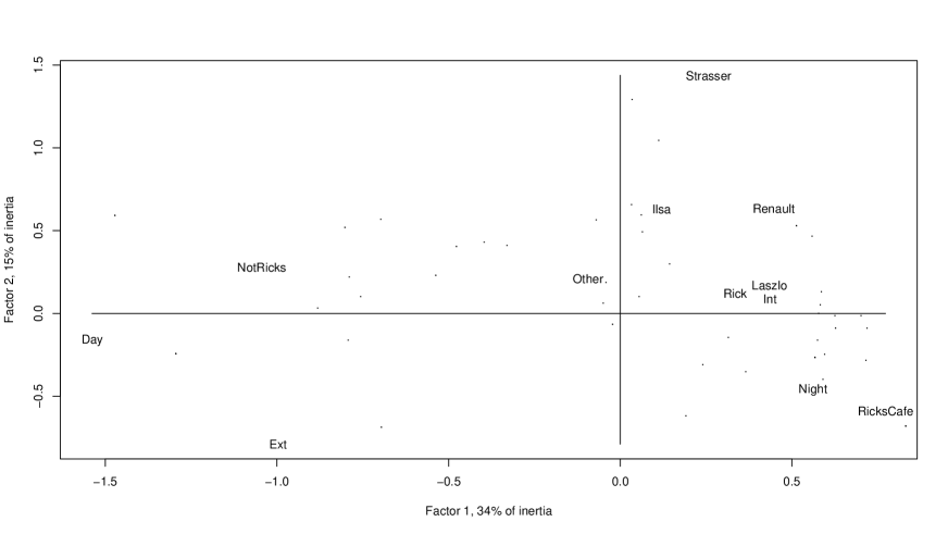
Figure 2: Correspondence Analysis of the Casablanca data derived from the script. The input data is presences/absences for 77 scenes crossed by 12 attributes. The 77 scenes are located at the dots, which are not labelled here for clarity. For a short review of the analysis methodology, see Appendix.

1.5 Modelling Semantics via the Geometry and Topology of Information

Some underlying principles are as follows. We start with the cross-tabulation data, scenes $\times$ attributes. Scenes and attributes are embedded in a metric space. This is how we are probing the geometry of information, which is a term and viewpoint used by [10].

Underpinning the display in Figure 2 is a Euclidean embedding. The triangular inequality holds for metrics. An example of a metric is the Euclidean distance, exemplified in Figure 3, where each and every triplet of points satisfies the relationship: $d(x,z)\leq d(x,y)+d(y,z)$ for distance $d$. Two other relationships also must hold. These are symmetry and positive definiteness, respectively: $d(x,y)=d(y,x)$, and $d(x,y)>0$ if $x\neq y$, $d(x,y)=0$ if $x=y$.

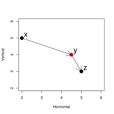
Figure 3: The triangular inequality defines a metric: every triplet of points satisfies the relationship: $d(x,z)\leq d(x,y)+d(y,z)$ for distance $d$.

Further underlying principles used in Figure 2 are as follows. The axes are the principal axes of momentum. Identical principles are used as in classical mechanics. The scenes are located as weighted averages of all associated attributes; and vice versa.

Figure 4: Depiction of Christiaan Huyghens, 1629–1695, from [1]. Towards the bottom on the right there is a depiction of the decomposition of the inertia of a hyperellipsoid cloud.

Huyghens’ theorem (cf. Figure 4) relates to decomposition of inertia of a cloud of points. This is the basis of Correspondence Analysis.

We come now to a different principle: that of the topology of information. The particular topology used is that of hierarchy. Euclidean embedding provides a very good starting point to look at hierarchical relationships. An innovation in our work is as follows: the hierarchy takes sequence, e.g. timeline, into account. This captures, in a more easily understood way, the notions of novelty, anomaly or change.

Let us take an informal case study to see how this works. Consider the situation of seeking documents based on titles. If the target population has at least one document that is close to the query, then this is (let us assume) clearcut. However if all documents in the target population are very unlike the query, does it make any sense to choose the closest? Whatever the answer here we are focusing on the inherent ambiguity, which we will note or record in an appropriate way. Figure 5 illustrates this situation, where the query is the point to the right.

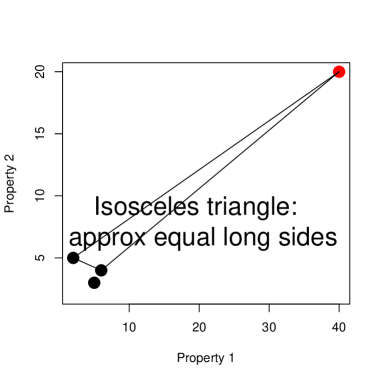
Figure 5: The query is on the far right. While we can easily determine the closest target (among the three objects represented by the dots on the left), is the closest really that much different from the alternatives?

By using approximate similarity this situation can be modelled as an isosceles triangle with small base, as illustrated in Figure 5. An ultrametric space has properties that are very unlike a metric space, and one such property is that the only triangles allowed are either (i) equilateral, or (ii) isosceles with small base. So Figure 5 can be taken as representing a case of ultrametricity. What this means is that the query can be viewed as having a particular sort of dominance or hierarchical relationship vis-à-vis any pair of target documents. Hence any triplet of points here, one of which is the query (defining the apex of the isosceles, with small base, triangle), defines local hierarchical or ultrametric structure. (See [6] for case studies.)

It is clear from Figure 5 that we should use approximate equality of the long sides of the triangle. The further away the query is from the other data then the better is this approximation [6].

What sort of explanation does this provide for our conundrum? It means that the query is a novel, or anomalous, or unusual “document”. It is up to us to decide how to treat such new, innovative cases. It raises though the interesting perspective that here we have a way to model and subsequently handle the semantics of anomaly or innocuousness.

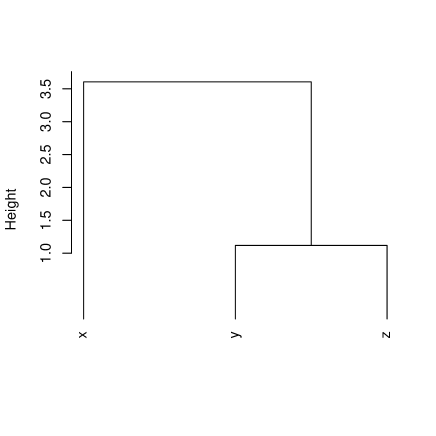
Figure 6: The strong triangular inequality defines an ultrametric: every triplet of points satisfies the relationship: $d(x,z)\leq\mbox{max}\{d(x,y),d(y,z)\}$ for distance $d$. Cf. by reading off the hierarchy, how this is verified for all $x,y,z$: $d(x,z)=3.5;d(x,y)=3.5;d(y,z)=1.0$. In addition the symmetry and positive definiteness conditions hold for any pair of points.

The strong triangular inequality, or ultrametric inequality, holds for tree distances: see Figure 6. The closest common ancestor distance is such an ultrametric.

1.6 Casablanca Narrative: Illustrative Analysis Continued

Figure 7 uses a sequence-constrained complete link agglomerative algorithm. It shows up scenes 9 to 10, and progressing from 39, to 40 and 41, as major changes. The sequence constrained algorithm, i.e. agglomerations are permitted between adjacent segments of scenes only, is described in an Appendix to this article, and in greater detail in [7]. The agglomerative criterion used, that is subject to this sequence constraint, is a complete link one.

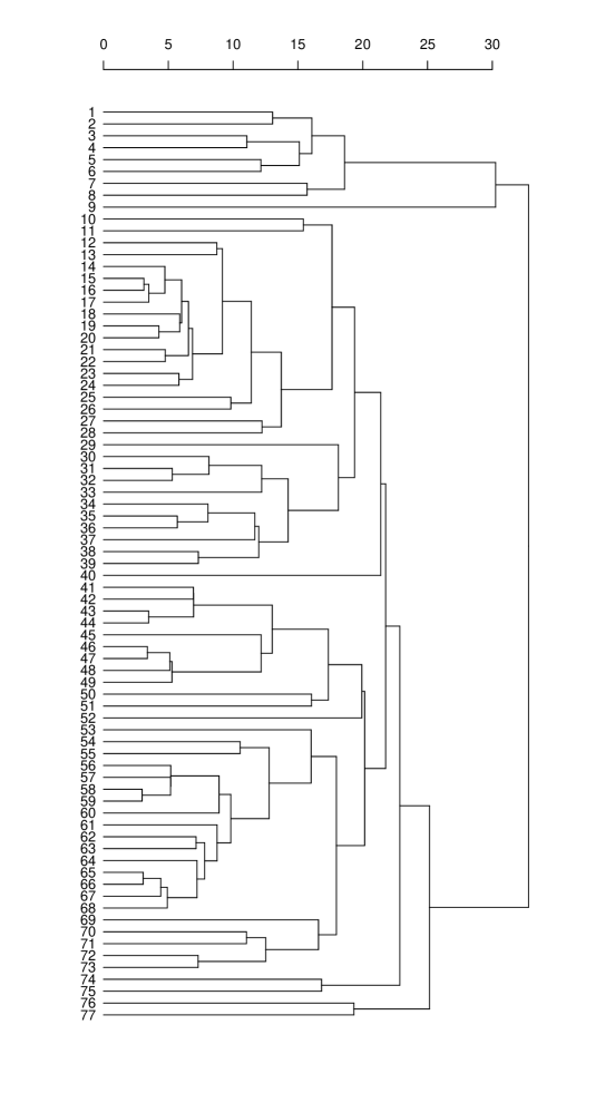
Figure 7: 77 scenes clustered. These scenes are in sequence: a sequence-constrained agglomerative criterion is used for this. The agglomerative criterion itself is a complete link one. See [5] for properties of this algorithm.

1.7 Our Platform for Analysis of Semantics

Correspondence analysis supports the following:

• analysis of multivariate, mixed numerical/symbolic data

• web of interrelationships

• evolution of relationships over time

Correspondence Analysis is in practice a tale of three metrics [7]. The analysis is based on embedding a cloud of points from a space governed by one metric into another. Furthermore the cloud offers vantage points of both observables and their characterizations, so – in the case of film script – for any one of the metrics we can effortlessly pass between the space of filmscript scenes and attribute set. The three metrics are as follows.

• Chi squared, $\chi^{2}$, metric – appropriate for profiles of frequencies of occurrence.

• Euclidean metric, for visualization, and for static context.

• Ultrametric, for hierarchic relations and, as we use it in this work, for dynamic context.

In the analysis of semantics, we distinguish two separate aspects.

1. Context – the collection of all interrelationships.

   • The Euclidean distance makes a lot of sense when the population is homogeneous.

   • All interrelationships together provide context, relativities – and hence meaning.

2. Hierarchy tracks anomaly.

   • Ultrametric distance makes a lot of sense when the observables are heterogeneous, discontinuous.

   • The latter is especially useful for determining: anomalous, atypical, innovative cases.

2 Deeper Look at Semantics of Casablanca

2.1 Text Data Mining

The Casablanca script has 77 successive scenes. In total there are 6710 words in these scenes. We define words as consisting of at least two letters. Punctuation is first removed. All upper case is set to lower case. We use from now on all words. We analyze frequencies of occurrence of words in scenes, so the input is a matrix crossing scenes by words.

2.2 Analysis of a Pivotal Scene, Scene 43

As a basis for a deeper look at Casablanca we have taken comprehensive but qualitative discussion by McKee [4] and sought quantitative and algorithmic implementation.

Casablanca is based on a range of miniplots. For McKee its composition is “virtually perfect”.

Following McKee [4] we will carry out an analysis of Casablanca’s “Mid-Act Climax”, Scene 43, subdivided into 11 “beats”. McKee divides this scene, relating to Ilsa and Rick seeking black market exit visas, into 11 “beats”.

1. Beat 1 is Rick finding Ilsa in the market.

2. Beats 2, 3, 4 are rejections of him by Ilsa.

3. Beats 5, 6 express rapprochement by both.

4. Beat 7 is guilt-tripping by each in turn.

5. Beat 8 is a jump in content: Ilsa says she will leave Casablanca soon.

6. In beat 9, Rick calls her a coward, and Ilsa calls him a fool.

7. In beat 10, Rick propositions her.

8. In beat 11, the climax, all goes to rack and ruin: Ilsa says she was married to Laszlo all along. Rick is stunned.

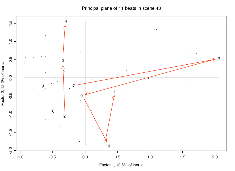
Figure 8: Correspondence Analysis principal plane – best Euclidean embedding in two dimensions – of scene 43. This scene is a central and indeed a pivotal one in the movie Casablanca. It consists of eleven sub-scenes, which McKee terms “beats”. We discuss in the text the evolution over sub-scenes 2, 3 and 4; and again over sub-scenes 7, 8, 9, 10, and 11.

Figure 8 shows the evolution from beat to beat rather well. 210 words are used in these 11 “beats” or subscenes. Beat 8 is a dramatic development. Moving upwards on the ordinate (factor 2) indicates distance between Rick and Ilsa. Moving downwards indicates rapprochement.

In the full-dimensional space we can check some other of McKee’s guidelines. Lengths of beat get shorter leading up to climax: word counts of final five beats in scene 43 are: 50 – 44 – 38 – 30 — 46. A style analysis of scene 43 based on McKee can be Monte Carlo tested against 999 uniformly randomized sets of the beats. In the great majority of cases (against 83% and more of the randomized alternatives) we find the style in scene 43 to be characterized by: small variability of movement from one beat to the next; greater tempo of beats; and high mean rhythm.

The planar representation in Figure 8 accounts for approximately 12.6% + 12.2% = 24.8% of the inertia, and hence the total information. We will look at the evolution of this scene, scene 43, using hierarchical clustering of the full-dimensional data – but based on the relative orientations, or correlations with factors. This is because of what we have found in Figure 8, viz. change of direction is most important.

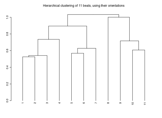
Figure 9: Hierarchical clustering of sequence of beats in scene 43 of Casablanca. Again, a sequence-constrained complete link agglomerative clustering algorithm is used. The input data is based on the full dimensionality Euclidean embedding provided by the Correspondence Analysis. The relative orientations (defined by correlations with the factors) are used as input data.

Figure 9 shows the hierarchical clustering, based on the sequence of beats. Input data are of full dimensionality so there is no approximation involved. Note the caesura in moving from beat 7 to 8, and back to 9. There is less of a caesura in moving from 4 to 5 but it is still quite pronounced.

Further discussion of these results can be found in [8].

3 Application of Narrative Analysis to Science and Engineering Policy

Our way of analyzing semantics is sketched out as follows:

• We discern story semantics arising out of the orientation of narrative.

• This is based on the web of interrelationships.

• We examine caesuras and breakpoints in the flow of narrative.

Let us look at the implications of this for data mining with decision policy support in view.

Consider a fairly typical funded project, and its phases up to and beyond the funding decision. Different research funding agencies differ in their procedures. But a narrative can always be strung together. All stages of the proposal and successful project life cycle, including external evaluation and internal decision making, are highly document – and as a consequence narrative – based. It is precisely the analysis of such a narrative that is our longer term goal.

As a first step towards much fuller analysis of these many and varied narratives involved in funded projects, let us look at the very general role of narrative in national research development. We will look at:

• Overall view – overall synthesis of information

• Orientation of strands of development

• Their tempo, rhythm

Through such an analysis of narrative, among the issues to be addressed are:

• Strategy and its implementation in terms of themes and subthemes represented

• Thematic focus and coverage

• Organisational clustering

• Evaluation of outputs in a global context

• All the above over time

Our aim is to understand the “big picture”. It is not to replace the varied measures of success that are applied, such as publications, patents, licences, numbers of PhDs completed, company start-ups, and so on. It is instead to appreciate the broader configuration and orientation, and to determine the most salient aspects underlying the data.

3.1 Assessing Coverage and Completeness

SFI Centres for Science, Engineering and Technology (CSETs) are campus-industry partnerships typically funded at up to €20 million over 5 years. Strategic Research Clusters (SRCs) are also research consortia, with industrial partners and over 5 years are typically funded at up to €7.5 million.

We cross-tabulated 8 CSETs and 12 SRCs by a range of terms derived from title and summary information; together with budget, numbers of PIs (Principal Investigators), Co-Is (Co-Investigators), and PhDs.

We can display any or all of this information on a common map, for visual convenience a planar display, using Correspondence Analysis.

In mapping SFI CSETs and SRCs, we will now show how Correspondence Analysis is based on the upper (near root) part of an ontology or concept hierarchy. This we view as information focusing. Correspondence Analysis provides simultaneous representation of observations and attributes. Retrospectively, we can project other observations or attributes into the factor space: these are supplementary observations or attributes. A 2-dimensional or planar view is likely to be a gross approximation of the full cloud of observations or of attributes. We may accept such an approximation as rewarding and informative. Another way to address this same issue is as follows. We define a small number of aggregates of either observations or attributes, and carry out the analysis on them. We then project the full set of observations and attributes into the factor space. For mapping of SFI CSETs and SRCs a simple algebra of themes as set out in the next paragraph achieves this goal. The upshot is that the 2-dimensional or planar view is a better fit to the full cloud of observations or of attributes.

From CSET or SRC characterization as: Physical Systems (Phys), Logical Systems (Log), Body/Individual, Health/Collective, and Data & Information (Data), the following thematic areas were defined.

1. eSciences = Logical Systems, Data & Information

2. Biosciences = Body/Individual, Health/Collective

3. Medical = Body/Individual, Health/Collective, Physical Systems

4. ICT = Physical Systems, Logical Systems, Data & Information

5. eMedical = Body/Individual, Health/Collective, Logical Systems

6. eBiosciences = Body/Individual, Health/Collective, Data & Information

This categorization scheme can be viewed as the upper level of a concept hierarchy. It can be contrasted with the somewhat more detailed scheme that we used for analysis of articles in the Computer Journal, [9].

CSETs labelled in the Figures are: APC, Alimentary Pharmabiotic Centre; BDI, Biomedical Diagnostics Institute; CRANN, Centre for Research on Adaptive Nanostructures and Nanodevices; CTVR, Centre for Telecommunications Value-Chain Research; DERI, Digital Enterprise Research Institute; LERO, Irish Software Engineering Research Centre; NGL, Centre for Next Generation Localization; and REMEDI, Regenerative Medicine Institute.

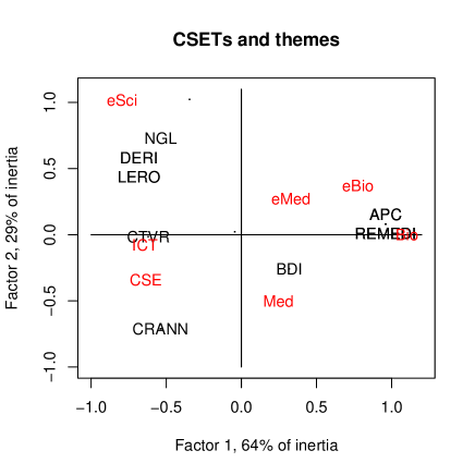
Figure 10: CSETs, labelled, with themes located on a planar display, which is nearly complete in terms of information content.

In Figure 10 eight CSETs and major themes are shown. Factor 1 counterposes computer engineering (left) to biosciences (right). Factor 2 counterposes software on the positive end to hardware on the negative end. This 2-dimensional map encapsulates 64% (for factor 1) + 29% (for factor 2) = 93% of all information, i.e. inertia, in the dual clouds of points. CSETs are positioned relative to the thematic areas used. In Figure 11, sub-themes are additionally projected into the display. This is done by taking the sub-themes as supplementary elements following the analysis as such: see Appendix for a short introduction to this. From Figure 11 we might wish to label additionally factor 2 as a polarity of data and physics, associated with the extremes of software and hardware.

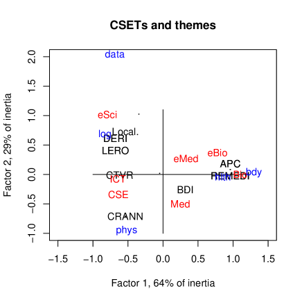
Figure 11: As Figure 10 but with sub-themes projected into the display. Note that, through use of supplementary elements, the axes and scales are identical to Figures 10, 12, and 13. Axes and scales are just displayed differently in this figure so that sub-themes appear in our field of view.

In Figure 12 CSET budgets are shown, as € million over 5 years, and themes are also displayed. In this way we use the map to show characteristics of the CSETs, in this case budgets.

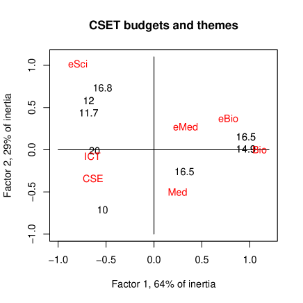
Figure 12: Similar to Figure 10, but here we show CSET budgets.

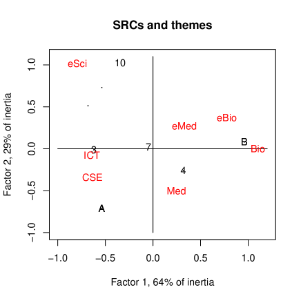
Figure 13: Using the same themes, the SRCs are projected. The properties of the planar display are the same as for Figures 10–12. SRCs 3, 4, 7, 10 are shown; and overlapping groups of 4 each are at A, B. A represents four bioscience or pharmaceutical SRCs. B represents four materials, biomaterials, or photonics SRCs. CSETs are displayed as dots (to avoid overcrowding of labels).

Figure 13 shows 12 SRCs (Strategic Research Clusters) that started at the end of 2007. The planar space into which the SRCs are projected is identical to Figures 10–12. This projection is accomplished by supplementary elements (see Appendix).

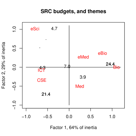
Figure 14: As Figure 13, now displaying combined budgets.

Figure 14 shows one property of the SRCs, their budgets in € million over 5 years.

3.2 Change Over Time

We take another funding programme, the Research Frontiers Programme, to show how changes over time can be mapped.

This programme follows an annual call, and includes all fields of science, mathematics and engineering. There are approximately 750 submissions annually. There was a 24% success rate (168 awards) in 2007, and 19% (143 awards) in 2008. The average award was €155k in 2007, and €161k in 2008. An award runs for three years of funding, and this is moving to four years in 2009 to accommodate a 4-year PhD duration.

We will look at the Computer Science panel results only, over 2005, 2006, 2007 and 2008.

Grants awarded in these years, respectively, were: 14, 11, 15, 17. The breakdown by institutes concerned was: UCD – 13; TCD – 10; DCU – 14; UCC – 6; UL – 3; DIT – 3; NUIM – 3; WIT – 1. These institutes are as follows: UCD, University College Dublin; DCU, Dublin City University; UCC, University College Cork; UL, University of Limerick; NUIM, National University of Ireland, Maynooth; DIT, Dublin Institute of Technology; and WIT, Waterford Institute of Technology.

One theme was used to characterize each proposal from among the following: bioinformatics, imaging/video, software, networks, data processing & information retrieval, speech & language processing, virtual spaces, language & text, information security, and e-learning. Again this categorization of computer science can be contrasted with one derived for articles in recent years in the Computer Journal [9].

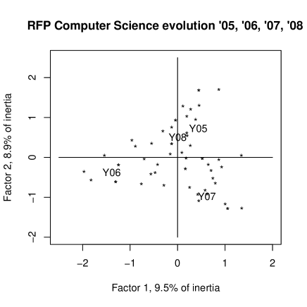
Figure 15: Research Frontiers Programme over four years. Successful proposals are shown as asterisks. The years are located as the average of successful projects.

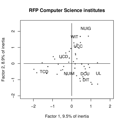
Figure 16: As Figure 15, displaying host institutes of the awardees.

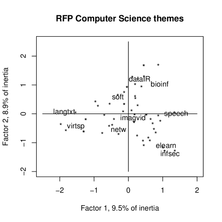
Figure 17: As Figures 15 and 16, displaying themes.

Figures 15, 16 and 17 show different facets of the Computer Science outcomes. By keeping the displays separate, we focus on one aspect at a time. All displays however are based on the same list of themes, and so allow mutual comparisons. Note that the principal plane shown accounts for 9.5% + 8.9% of the inertia, hence 18.4% of the overall inertia, that in turn expresses information here. Although small, it is the best planar view of the data (arising from the $\chi^{2}$ or chi squared metric, see Appendix, followed by the Euclidean embedding that the figures show). Ten themes were used, and what the 18.4% information content tells us is that there is importance attached to most if not all of the ten. We are not prevented though in studying usefully the planar displays. That they can be used to display lots of supplementary data is a major benefit of their use.

What our analyses demonstrate is that the categories used are of crucial importance. Indeed, in Figures 10–14 and then in Figures 15–17, we see how we can “engineer” the impact of the categories by assimilating their importance to moments of inertia of the clouds of associated points.

3.3 Conclusion on the Policy Case Studies

The aims and objectives in our use of the Correspondence Analysis and clustering platform is to drive strategy and its implementation in policy.

What we are targeting is to study highly multivariate, evolving data flows. This is in terms of the semantics of the data – principally, complex webs of interrelationships and evolution of relationships over time. This is the narrative of process that lies behind raw statistics and funding decisions.

We have been concerned especially with information focusing in section 3.1, and this over time in section 3.2.

4 Conclusions

Data collected on processes or configurations can tell us a lot about what is going on. When backed up with probabilistic models, we can test one hypothesis against another. This leads to data mining “in the small”. Pairwise plots are often sufficient because as visualizations they remain close and hence faithful to the original data. Such data mining “in the small” is well served by statistics as a discipline.

Separately from such data mining “in the small”, there is a need for data mining “in the large”. We need to unravel the broad brush strokes of narrative expressing a story. Indeed as discussed in [3], narrative expresses not just a story but human thinking. A broad brush view of science and engineering research, and their linkages with the economy, is a similar type of situation. Pairwise plots are not always sufficient now, because they tie us down in unnecessary detail. We use them since we need the more important patterns, trends, details to be brought out in order of priority. Strategy is of the same class as narrative.

For data mining “in the large” the choice of data and categorization used are crucial. This we have exemplified well in this article. So our data mining “in the large” is tightly coupled to the data. This is how we can make data speak. The modelling involved in analysis “in the small” comes later.

Appendix: the Correspondence Analysis and Hierarchical Clustering Platform

This Appendix introduces important aspects of Correspondence Analysis and hierarchical clustering. Further reading is to be found in [1] and [7].

Analysis Chain

1. Starting point: a matrix that cross-tabulates the dependencies, e.g. frequencies of joint occurrence, of an observations crossed by attributes matrix.

2. By endowing the cross-tabulation matrix with the $\chi^{2}$ metric on both observation set (rows) and attribute set (columns), we can map observations and attributes into the same space, endowed with the Euclidean metric.

3. A hierarchical clustering is induced on the Euclidean space, the factor space.

4. Interpretation is through projections of observations, attributes or clusters onto factors. The factors are ordered by decreasing importance.

Various aspects of Correspondence Analysis follow on from this, such as Multiple Correspondence Analysis, different ways that one can encode input data, and mutual description of clusters in terms of factors and vice versa. In the following we use elements of the Einstein tensor notation of [1]. This often reduces to common vector notation.

Correspondence Analysis: Mapping $\chi^{2}$ Distances into Euclidean Distances

• The given contingency table (or numbers of occurrence) data is denoted $k_{IJ}=\{k_{IJ}(i,j)=k(i,j);i\in I,j\in J\}$.

• $I$ is the set of observation indexes, and $J$ is the set of attribute indexes. We have $k(i)=\sum_{j\in J}k(i,j)$. Analogously $k(j)$ is defined, and $k=\sum_{i\in I,j\in J}k(i,j)$.

• Relative frequencies: $f_{IJ}=\{f_{ij}=k(i,j)/k;i\in I,j\in J\}\subset\mathbb{R}_{I\times J}$, similarly $f_{I}$ is defined as $\{f_{i}=k(i)/k;i\in I,j\in J\}\subset\mathbb{R}_{I}$, and $f_{J}$ analogously.

• The conditional distribution of $f_{J}$ knowing $i\in I$, also termed the $j$th profile with coordinates indexed by the elements of $I$, is:

  $$f^{i}_{J}=\{f^{i}_{j}=f_{ij}/f_{i}=(k_{ij}/k)/(k_{i}/k);f_{i}>0;j\in J\}$$

  and likewise for $f^{j}_{I}$.

• What is discussed in terms of information focusing in the text is underpinned by the principle of distributional equivalence. This means that if two or more profiles are aggregated by simple element-wise summation, then the $\chi^{2}$ distances relating to other profiles are not effected.

Input: Cloud of Points Endowed with the Chi Squared Metric

• The cloud of points consists of the couples: (multidimensional) profile coordinate and (scalar) mass. We have $N_{J}(I)=$ $\{(f^{i}_{J},f_{i});i\in I\}\subset\mathbb{R}_{J}$, and again similarly for $N_{I}(J)$.

• Included in this expression is the fact that the cloud of observations, $N_{J}(I)$, is a subset of the real space of dimensionality $|J|$ where $|.|$ denotes cardinality of the attribute set, $J$.

• The overall inertia is as follows:

  $$M^{2}(N_{J}(I))=M^{2}(N_{I}(J))=\|f_{IJ}-f_{I}f_{J}\|^{2}_{f_{I}f_{J}}$$

  $$=\sum_{i\in I,j\in J}(f_{ij}-f_{i}f_{j})^{2}/f_{i}f_{j}$$

• The term $\|f_{IJ}-f_{I}f_{J}\|^{2}_{f_{I}f_{J}}$ is the $\chi^{2}$ metric between the probability distribution $f_{IJ}$ and the product of marginal distributions $f_{I}f_{J}$, with as centre of the metric the product $f_{I}f_{J}$.

• Decomposing the moment of inertia of the cloud $N_{J}(I)$ – or of $N_{I}(J)$ since both analyses are inherently related – furnishes the principal axes of inertia, defined from a singular value decomposition.

Output: Cloud of Points Endowed with the Euclidean Metric in Factor Space

• The $\chi^{2}$ distance with centre $f_{J}$ between observations $i$ and $i^{\prime}$ is written as follows in two different notations:

  $$d(i,i^{\prime})=\|f^{i}_{J}-f^{i^{\prime}}_{J}\|^{2}_{f_{J}}=\sum_{j}\frac{1}{f_{j}}\left(\frac{f_{ij}}{f_{i}}-\frac{f_{i^{\prime}j}}{f_{i^{\prime}}}\right)^{2}$$

• In the factor space this pairwise distance is identical. The coordinate system and the metric change.

• For factors indexed by $\alpha$ and for total dimensionality $N$ ($N=\mbox{ min }\{|I|-1,|J|-1\}$; the subtraction of 1 is since the $\chi^{2}$ distance is centred and hence there is a linear dependency which reduces the inherent dimensionality by 1) we have the projection of observation $i$ on the $\alpha$th factor, $F_{\alpha}$, given by $F_{\alpha}(i)$:

  $$d(i,i^{\prime})=\sum_{\alpha=1..N}\left(F_{\alpha}(i)-F_{\alpha}(i^{\prime})\right)^{2}$$ (1)

• In Correspondence Analysis the factors are ordered by decreasing moments of inertia.

• The factors are closely related, mathematically, in the decomposition of the overall cloud, $N_{J}(I)$ and $N_{I}(J)$, inertias.

• The eigenvalues associated with the factors, identically in the space of observations indexed by set $I$, and in the space of attributes indexed by set $J$, are given by the eigenvalues associated with the decomposition of the inertia.

• The decomposition of the inertia is a principal axis decomposition, which is arrived at through a singular value decomposition.

Supplementary Elements: Information Space Fusion

Dual Spaces and Transition Formulas

• $$F_{\alpha}(i)=\lambda^{-\frac{1}{2}}_{\alpha}\sum_{j\in J}f^{i}_{j}G_{\alpha}(j)\mbox{ for }\alpha=1,2,\dots N;i\in I$$

  $$G_{\alpha}(j)=\lambda^{-\frac{1}{2}}_{\alpha}\sum_{i\in I}f^{j}_{i}F_{\alpha}(i)\mbox{ for }\alpha=1,2,\dots N;j\in J$$

• Transition formulas: The coordinate of element $i\in I$ is the barycentre of the coordinates of the elements $j\in J$, with associated masses of value given by the coordinates of $f^{i}_{j}$ of the profile $f^{i}_{J}$. This is all to within the $\lambda^{-\frac{1}{2}}_{\alpha}$ constant.

• In the output display, the barycentric principle comes into play: this allows us to simultaneously view and interpret observations and attributes.

Supplementary Elements

Overly-preponderant elements (i.e. row or column profiles), or exceptional elements (e.g. a sex attribute, given other performance or behavioural attributes) may be placed as supplementary elements. This means that they are given zero mass in the analysis, and their projections are determined using the transition formulas. This amounts to carrying out a Correspondence Analysis first, without these elements, and then projecting them into the factor space following the determination of all properties of this space.

Here too we have a new approach to fusion of information spaces focusing the projection.

Hierarchical Clustering

Background on hierarchical clustering in general, and the particular algorithm used here, can be found in [5].

Consider the projection of observation $i$ onto the set of all factors indexed by $\alpha$, $\{F_{\alpha}(i)\}$ for all $\alpha$, which defines the observation $i$ in the new coordinate frame. This new factor space is endowed with the (unweighted) Euclidean distance, $d$. We seek a hierarchical clustering that takes into account the observation sequence, i.e. observation $i$ precedes observation $i^{\prime}$ for all $i,i^{\prime}\in I$. We use the linear order on the observation set.

Agglomerative hierarchical clustering algorithm:

1. Consider each observation in the sequence as constituting a singleton cluster. Determine the closest pair of adjacent observations, and define a cluster from them.

2. Determine and merge the closest pair of adjacent clusters, $c_{1}$ and $c_{2}$, where closeness is defined by $d(c_{1},c_{2})=\mbox{ max }\{d_{ii^{\prime}}$ $\mbox{ such that }i\in c_{1},i^{\prime}\in c_{2}\}$.

3. Repeat the second step until only one cluster remains.

This is a sequence-constrained complete link agglomeration criterion. The cluster proximity at each agglomeration is strictly non-decreasing.

References

- [1] J.-P. Benzécri, L’Analyse des Données, Tome I Taxinomie, Tome II Correspondances, 2nd ed. Dunod, Paris, 1979.
- [2] M. Burnett and J. Allison, Everybody Comes to Rick’s, screenplay, 1940.
- [3] W.L. Chafe, The flow of thought and the flow of language, In Syntax and Semantics: Discourse and Syntax, ed. by Talmy Givón, vol. 12, 159–181, Academic Press, 1979.
- [4] R. McKee, Story: Substance, Structure, Style, and the Principles of Screenwriting, Methuen, 1999.
- [5] F. Murtagh, Multidimensional Clustering Algorithms, Physica-Verlag, Würzburg, 1985.
- [6] F. Murtagh, On ultrametricity, data coding, and computation, Journal of Classification, 21, 167-184, 2004.
- [7] F. Murtagh, Correspondence Analysis and Data Coding with R and Java, Chapman & Hall/CRC, 2005.
- [8] F. Murtagh, A. Ganz and S. McKie, The structure of narrative: the case of film scripts, Pattern Recognition, in press, 2008. http://dx.doi.org/10.1016/j.patcog.2008.05.026 (Discussed in: Z. Merali, Here’s looking at you, kid. Software promises to identify blockbuster scripts, Nature, 453, 708, 4 June 2008.)
- [9] F. Murtagh, Editorial, Computer Journal, in press, 2008. doi:10.1093/comjnl/bxn008
- [10] C.J. van Rijsbergen, The Geometry of Information Retrieval, Cambridge University Press, 2004.