Semi-flexible hydrogen-bonded and non-hydrogen bonded lattice polymers

Abstract

We investigate the addition of stiffness to the lattice model of hydrogen-bonded polymers in two and three dimensions. We find that, in contrast to polymers that interact via a homogeneous short-range interaction, the collapse transition is unchanged by any amount of stiffness: this supports the physical argument that hydrogen bonding already introduces an effective stiffness. Contrary to possible physical arguments, favouring bends in the polymer does not return the model’s behaviour to that comparable to the semi-flexible homogeneous interaction model, where the canonical $\theta$-point occurs for a range of parameter values. In fact, for sufficiently large bending energies the crystal phase disappears altogether, and no phase transition of any type occurs. We also compare the order-disorder transition from the globule phase to crystalline phase in the semi-flexible homogeneous interaction model to that for the fully-flexible hybrid model with both hydrogen and non-hydrogen like interactions. We show that these phase transitions are of the same type and are a novel polymer critical phenomena in two dimensions. That is, it is confirmed that in two dimensions this transition is second-order, unlike in three dimensions where it is known to be first order. We also estimate the crossover exponent and show that there is a divergent specific heat, finding $\phi=0.7(1)$ or equivalently $\alpha=0.6(2)$. This is therefore different from the $\theta$ transition, for which $\alpha=-1/3$.

1 Introduction

When modelling a single polymer in dilute solution by a lattice self-avoiding walk [1, 2, 3] the effects of solvent mediated intra-polymer interaction are often included by assigning an energy to each non-consecutive pair of monomers lying on the neighbouring lattice sites: the interaction is homogeneous in that in doesn’t depend on shape of the two parts of the polymer containing the interacting monomers. This is the well-studied Interacting self-avoiding walk (ISAW) model which is the standard model of polymer collapse using self-avoiding walks. If the energy is repulsive the polymer behaves as a swollen chain (the so-called excluded-volume state) regardless of temperature and one says that it is in a good solvent. When the energy is attractive, and the temperature is low enough, the chain becomes a rather more compact globule [2, 4], reminiscent of a liquid droplet: this is also known as the poor solvent situation. The transition point between these two phases is called the $\theta$-point; it is a well studied continuous phase transition (see [5] and references therein). However, the mapping of monomers onto lattice sites ignores the natural rigidity of real polymers. An energy for bends in the self-avoiding walk can be introduced to take account of this feature. The model of semi-flexible polymers has been investigated mostly in three dimensions [6, 7, 8]. In particular, Bastolla and Grassberger [6] investigated semi-flexible interacting self-avoiding walks (semiflexible ISAW) on the cubic lattice, which interact via all nearest-neighbours, as in the $\theta$-point model, and included the bending energy. They showed that when there is a strong energetic preference for straight segments, this model undergoes a single first-order transition from the excluded-volume high-temperature state to a crystalline state. Intriguingly, if there is only a weak preference for straight segments, the polymer undergoes two phase transitions: on lowering the temperature the polymers undergoes the $\theta$-point transition to the liquid globule followed at a lower temperature by a first-order transition to the frozen crystalline phase. In two dimensions the transition between the globule and the frozen state has been studied in Hamiltonian walks, and there it seems to be a continuous one [9].

The modelling of polymers in solution changes as soon as we want to describe any biological system (e.g. proteins), in which the hydrogen bonding plays an important role [10]. One of the main features of the bonding is that the interacting residua lie on a partially straight segments of the chain. Hydrogen-like bonding was first modelled on the cubic and square lattices using Hamiltonian paths by Bascle et al. [11]. A monomer acquires a hydrogen-like bond with its (non-consecutive) nearest neighbour if both of them lie on straight sections of the chain. Note that the identification of a single contact of this type with a single hydrogen bond is only valid if fully-flexible polymers are considered; otherwise the contact represents an agglomeration of such bonds. The interacting self-avoiding walk modified to have only such interactions will be referred to as the hydrogen-like bonding model, or rather IHB model. The IHB model was studied in mean-field approximation [11] and a first-order transition from a high-temperature excluded-volume (swollen) phase to a quasi-frozen solid-like phase was found in both two and three dimensions. Hence this would indicate that it is a different type of transition from the $\theta$-point. Note also that the low temperature phase was found to be anisotropic whereas the collapsed globule of the standard $\theta$-point model is isotropic. The IHB model on the square lattice was studied directly by Foster and Seno by means of the transfer matrix method [12] and by Krawczyk et al. [13] on both the square and cubic lattice using a Monte Carlo method. In both of these studies a first-order transition was found between an excluded-volume (swollen-coil) state and an anisotropic ordered compact phase in two and in three dimensions, again in opposition to the $\theta$-point [2].

However, the IHB model was recently extended [14] to a hybrid model (IHB–INH) that includes both the hydrogen-like bond interactions and non-hydrogen like bond interactions, with separate energy parameters. When the non-hydrogen bonding energy is set to zero the IHB model is recovered. If both energies are set to be the same then the ISAW without stiffness is recovered. For large values of the ratio of the interaction strength of hydrogen-bonds to non-hydrogen bonds, a polymer will undergo a single first-order phase transition from a swollen coil at high temperatures to a folded crystalline state at low temperatures. On the other hand, for any ratio of these interaction energies less than or equal to one there is a single $\theta$-like transition from a swollen coil to a liquid droplet-like globular phase. Importantly, for intermediate ratios two transitions can occur, so that the polymer first undergoes a $\theta$-like transition on lowering the temperature, followed by a second transition to the crystalline state. In three dimensions it was found that this second transition is first order, while in two dimensions it is probably second order with a divergent specific heat. In other words, at least in three dimensions, by adding an energy to both the hydrogen-like and non-hydrogen like interactions a phase diagram similar to the one for the semi-flexible ISAW is obtained.

Various issues then arise. Firstly it is worth studying the addition of stiffness to the IHB model since stiffness clearly affects the type of phases that occur in the ISAW model. Moreover, one could argue that since in the IHB model interactions occur only between straight segments of the walk, an effective stiffness has already been introduced: one could then go further and argue that favouring bends may result in behaviour like that in the ISAW model. Secondly, it is worth investigating the semi-flexible ISAW model in two dimensions to check if the similarity of the IHB–INH phase diagram to the semi-flexible ISAW extends to that dimension. In particular, given the existence of the same three phases (as we shall find) whether the globule-crystal transition is of the same second order type as in the IHB–INH model. Finally the more general relationship between these three potentials (nearest-neighbour interaction, hydrogen-like bonding and stiffness) on the phase structure of the model polymers is worth pursuing. Hence, in this paper we investigate via Monte Carlo simulations the effect of adding stiffness to the interacting hydrogen bonding model and compare this to adding stiffness to the canonical ISAW model. Intriguingly we find that favouring stiffness does not change the single transition found in the IHB model without stiffness. However, for a sufficiently large bending energy favouring bends the transition temperature is found to go to zero, and for larger ratios of bending energy to hydrogen bonding energy no phase transition occurs. We then compare the globule-crystal phase transition in the semi-flexible ISAW model on the square lattice (on the cubic lattice they are both first-order) to that of the IHB–INH model and show that the exponents are most likely the same: we also estimate these exponents.

In general we have considered various restrictions of a model of three parameters where stiffness is added to the hydrogen-bond interactions and non-hydrogen-bond interactions. In our conclusions we argue that only three phases exist in the larger parameter space: an excluded-volume dominated state (where the polymer is ‘swollen’), a disordered globular state where the polymer is in a condensed liquid-like drop and a crystalline state.

The paper is organised as follows. In Section 2 we explain more carefully details of the models considered. In Section 3 we consider the semi-flexible interacting hydrogen bond model. In Section 4 we consider the semi-flexible version of the canonical interacting SAW model and we compare our results to those from a model that has different energies for hydrogen and non-hydrogen nearest-neighbour interactions. In Section 5 we investigate a semi-flexible interacting polymer where there are no hydrogen bonds. We end with some conclusions about the most general model defined in Section 2.

2 Definitions

Let us define a general model that contains each of the models considered as sub-cases via restricting parameters.

We begin with a self-avoiding walk on the square and simple cubic lattices. The walk consists of a sequence of occupied lattice sites joined by steps of the walk. A walk of $n$ steps occupies $n+1$ sites. Consider the sites of the lattice occupied by the walk. When two sites of the walk are adjacent on the lattice and not consecutive along the walk, so as not to be joined by a step of the walk, we refer to this pair of sites as a nearest-neighbour contact. Additionally, let us refer to two consecutive steps that follow the same lattice direction as a stiff step-pair, so that there are three consecutive occupied sites along a line on the lattice, and the site in the centre of this trio to be a stiffness site (see Figure 1).

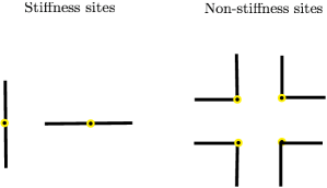
Figure 1: Stiffness sites and non stiffness sites on the square lattice

Now partition the possible types of contact into two classes: when they occur between stiffness sites then we refer to these as hydrogen-bond contacts, and all others are non-hydrogen-bond contacts. In Figure 2 the partition of the types of nearest-neighbour contacts for the square lattice is shown. In Figure 3 the hydrogen-bond contacts (only) are shown for the cubic lattice.

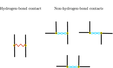
Figure 2: The partition of the types of nearest-neighbour contacts into hydrogen-bonds and non-hydrogen-bonds for the square lattice is shown. Rotations of these are also possible.

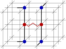
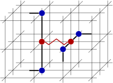
Figure 3: Hydrogen-bond contacts for the simple cubic lattices.

We now add an energy to the self-avoiding which consists of three contributions: an energy for each hydrogen-bond contact $-\varepsilon_{hb}$, an energy of non-hydrogen-bond contact $-\varepsilon_{nh}$ and an energy for stiff step-pairs $-\varepsilon_{ss}$. The total energy of a walk configuration $\varphi_{n}$ of $n$ steps is

$$E_{n}(\varphi_{n})=-m_{hb}(\varphi_{n})\ \varepsilon_{hb}-m_{nh}(\varphi_{n})\ \varepsilon_{nh}-m_{ss}(\varphi_{n})\ \varepsilon_{ss},$$ (2.1)

where $m_{hb}$ denotes the number of of hydrogen-bond contacts, $m_{nh}$ denotes the the number of non-hydrogen-bond contacts, and $m_{ss}$ denotes the number of stiffness sites in the walk configuration (see Figure 4).

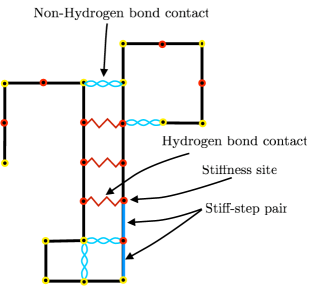
Figure 4: A sample walk configuration with the various type of interaction highlighted for the square lattice.

We will denote the total number of all nearest-neighbours interactions as $m_{is}$, where it is equal to the sum of the number of the two types of interaction considered in our full model, that is $m_{is}=m_{nh}+m_{hb}$.

The inverse temperature is denoted as $\beta=1/k_{B}T$, where $k_{B}$ is the Boltzmann constant and $T$ the absolute temperature. We define for convenience $\beta_{hb}=\beta\varepsilon_{hb}$, $\beta_{nh}=\beta\varepsilon_{nh}$ and $\beta_{ss}=\beta\varepsilon_{ss}$. The partition function is then given by

$$Z_{n}(\beta_{hb},\beta_{nh},\beta_{ss})=\sum_{m_{hb},m_{nh},m_{s}}C_{n,m_{hb},m_{nh},m_{ss}}\;e^{\beta_{hb}m_{hb}+\beta_{nh}m_{nh}+\beta_{ss}m_{ss}}$$ (2.2)

with $C_{n,m_{hb},m_{nh},m_{ss}}$ the density of states. Canonical averages are calculated with respect to this density of states.

Our results are for the following models:

• the semi-flexible interacting hydrogen-bonding model (semi-flexible IHB model) where $\beta_{nh}=0$,

• the semi-flexible interacting non-hydrogen-bonding model (semi-flexible INH model) where $\beta_{hb}=0$,

• and the semi-flexible interacting self-avoiding walk model (semi-flexible ISAW model) where $\beta_{hb}=\beta_{nh}$.

We remind the reader that the semi-flexible ISAW model on the simple cubic lattice has previously been studied by Bastolla and Grassberger [6].

We compare our results to those concerning the previously studied [14] model where different energies are assigned to hydrogen-bond contacts and non-hydrogen-bond contacts, though not to stiffness sites, namely

• the Interacting hydrogen-bonding – Interacting non-hydrogen-bonding model (IHB–INH model) where $\beta_{ss}=0$.

All the simulations in this paper use a Monte Carlo technique, known as FlatPERM [15], which is well suited to the study of self-avoiding walks on the simple cubic and square lattices with interactions. This technique allows for the estimation of quantities at all values of an interaction parameter by the estimation of the appropriate ‘density of states’: e.g. from equation (2.2) the estimation of $C_{n,m_{hb},m_{nh},m_{ss}}$ would allow the calculation of canonical averages for any value of the parameters $\beta_{hb}$, $\beta_{nh}$ and $\beta_{ss}$. On the other hand each new parameter increases the computational cost by at least a factor of $n$ (being the range of the variable — e.g. $m_{hb}$ when including $\beta_{hb}$). Therefore so as to obtain data for reasonable length walks it is necessary to restrict simulations to one or two interaction parameters.

3 Semi-flexible IHB model ($\beta_{nh}=0$)

We have simulated the semi-flexible IHB model on the square and simple cubic lattice, estimating an appropriate density of states $C_{n,m_{hb},m_{ss}}$, so that averages can be performed for all values of the parameters $\beta_{hb}$ and $\beta_{ss}$. We have estimated $\langle m_{hb}\rangle$ and $\langle m_{ss}\rangle$, which are directly related to the internal energy, and the variances in these averages which are related to the specific heat of the model. These ‘two parameter’ simulations were completed up to $n=128$ steps.

Let us start by considering the square lattice data. As has been previously found [12, 13] at $\beta_{ss}=0$, we find that for any fixed value of $\beta_{ss}$ there is strongly growing peak in the variance of $m_{hb}$ at a single value of $\beta_{hb}$. This is indicative of a phase transition at some position $\beta_{hb}^{(c)}(\beta_{ss})$ and as the normalised peak of the variance is growing close to linearly with $n$ irrespective of $\beta_{ss}$ it is indicative of a first order phase transition. To confirm this we considered the distribution of $m_{hb}$ at the finite-size transition point $\beta_{hb}^{(c)}(\beta_{ss};n)$. In Figure 5 we show this distribution at $\beta_{hb}^{(c)}(0.5;128)$, $\beta_{hb}^{(c)}(0.5;64)$ and $\beta_{hb}^{(c)}(-0.5;128)$, $\beta_{hb}^{(c)}(-0.5;64)$. The deepening bimodal distributions reinforce our conclusion that the transition is first order regardless of $\beta_{ss}$.

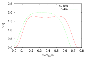
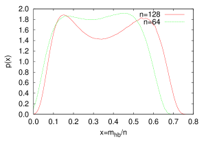
Figure 5: Distribution of internal energy for the square lattice semi-flexible IHB model at the estimated transition point $\beta_{hb}^{(c)}(\beta_{ss};n)$ when $\beta_{ss}=0.5$ (left), and $\beta_{ss}=-0.5$ (right), using $n=128$ and $n=64$.

By considering the scaling of the end-to-end distance and the anisotropy parameter (see [14]) we have verified that for $\beta_{hb}<<\beta_{hb}^{(c)}(\beta_{ss},n)$ the extended phase exists while for $\beta_{hb}>>\beta_{hb}^{(c)}(\beta_{ss},n)$ the anisotropic crystal phase is observed.

In Figure 6 a plot of $\beta_{hb}^{(c)}(\beta_{ss};128)$ is given in the two-dimensional space of $\beta_{hb}$, and $\beta_{ss}$. Next to that in Figure 6 the same curve is plotted in the three-dimensional space of $\beta_{hb}$, $\beta_{nh}$ and $\beta_{ss}$.

The results for the cubic lattice are completely analogous and the finite size phase diagram is given in Figure 7.

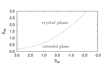
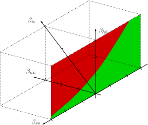
Figure 6: Plot of the finite size phase boundary for the semi-flexible IHB model on the square lattice (left). The plane of the parameters of the semi-flexible IHB model in the more general three parameter space: the two phases are denoted by a dark (red) shading for the crystalline phase and a mid-density (green) shading for the extended swollen polymer phase. (right)

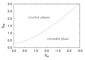
Figure 7: Plot of the finite size phase boundary for the semi-flexible IHB model on the cubic lattice

On both lattices we therefore have found that the addition of positive stiffness to the interacting hydrogen-like bond model leaves the single phase transition from a swollen phase at high temperatures to a crystalline phase at low temperatures unchanged. When favouring bends, so that $\varepsilon_{ss}$ and $\beta_{ss}$ are negative, then when any transition occurs it is again of a similar type as the fully-flexible model. However there is a range of $\lambda=\varepsilon_{ss}/\varepsilon_{hb}$ such that no transition occurs. This is relative easy to understand: hydrogen bonds only occur between two stiffness sites which are suppressed by large negative values of $\varepsilon_{ss}$. Let us focus on the square lattice. On the square lattice for $\lambda=\varepsilon_{ss}/\varepsilon_{hb}<-1$ no phase transition occurs on lowering the temperature. At zero temperatures the ground state for $\lambda<-1$ is a walk consisting only of bends with energy zero (this state should have a positive entropy). For $-1<\lambda$ the ground state is one with long folds ($\beta$-like sheets) and a bulk energy $-n(\varepsilon_{hb}+\varepsilon_{ss})$ which is negative so long as $\varepsilon_{hb}>-\varepsilon_{ss}$. This state has zero entropy. The difference in entropy accounts for the apparent shift of the asymptote of the phase boundary from $\beta_{hb}=-\beta_{ss}$ to $\beta_{hb}=-\beta_{ss}+c$ in Figure 6.

4 Semi-Flexible ISAW ($\beta_{nh}=\beta_{hb}$)

For the semi-flexible ISAW model we focus our attention on the square lattice which has not previously been investigated. On the square lattice we performed simulations for $n=128$ for two parameters $\beta_{is}$ and $\beta_{ss}$ as well as for the one parameter $\beta_{ss}$ for constant $\beta_{is}=0.7$ for lengths up to $n=512$. The line $\beta_{is}=0.7$ was chosen so as to focus on the transition between two collapsed phases: the collapsed-globule and the crystal.

Let us begin with the two parameter simulations. By considering the maximum eigenvalue of the matrix of fluctuations of $m_{is}$ and $m_{ss}$ we have mapped out a finite sized phase boundary, see Figure 8.

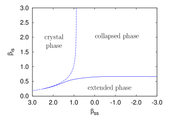
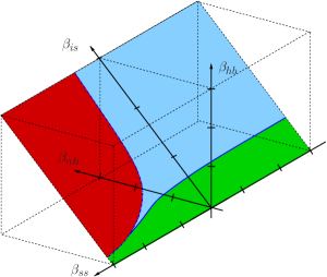
Figure 8: Plot of the finite size phase boundary for the semi-flexible ISAW model on the square lattice (top). The plane of the parameters of the semi-flexible ISAW model in the more general three parameter space: the three phases are denoted by a light (blue) shading for the globular phase, a mid-density (green) shading for the extended swollen polymer phase and a dark (red) shading for the crystalline phase. (bottom)

The boundaries clearly divide the phase space into three phases. Once again, by considering the scaling of various quantities such as the end-to-end distance at fixed points deep within each suspected phase we are satisfied that the three phases are the same as in the IHB–INH model [14] on the square lattice: a swollen phase with $\nu=3/4$, and two collapsed phases where $\nu=1/2$. In one phase the typical configurations are clearly anisotropic, looking like folded $\beta$-sheets, indicating that it is a crystalline phase. Hence the phase structure and phase diagram is similar to the three-dimensional case. We have attempted to locate the triple point which seems to around $(\beta_{ss},\beta_{is})=(2.0,0.3)$. However using different methods has resulted in quite different estimates so we do not propose any error estimate on these values.

For convenience and comparison the corresponding finite size phase boundary diagrams for the IHB–INH model studied by Krawczyk et al. [14] are given in Figure 9 .

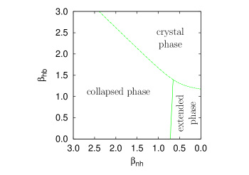
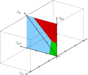
Figure 9: Plot of the finite size phase boundary for the fully-flexible IHB–INH model on the square lattice (top). The plane of the parameters of the semi-flexible INH model in the more general three parameter space: the three phases are denoted by a light (blue) shading for the globular phase, a mid-density (green) shading for the extended swollen polymer phase and a dark (red) shading for the crystalline phase (bottom).

Since the extended-globule $\theta$ transition has been well studied we have focussed on the two other transitions: extended-crystal and globule-crystal. Both these transitions are first order on the cubic lattice [6]. In the IHB–INH model [14] the extended-crystal was also first order on both the square and cubic lattice. So firstly let us consider this transition in the semi-flexible ISAW model on the square lattice. By considering the scaling of the fluctuations in $m_{ss}$ and the distribution of $m_{ss}$ we confirm that the first order nature of this transition. Figure 10 demonstrates that the data is consistent with first order scaling at the transition point of the swollen to crystal phases.

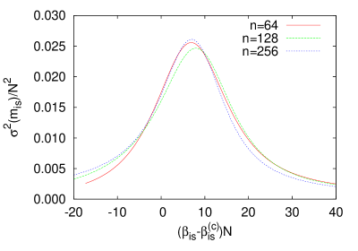
Figure 10: Plots of the fluctuations per monomer divided by $N$ in the number of ISAW contacts ($m_{is}$) at $\beta_{ss}=2.0$ for $2d$˛ with the horizontal axis scaled as (($\beta_{is}-\beta_{is}^{(c)})N$). We have used $\beta_{is}^{(c)}=0.27$. Shown are lengths $64$, $128$ and $256$.

In Figure 11 the maximum of fluctuations for the transition between the globule and crystalline phases for the semi-flexible and IHB–INH models are plotted together. The semi-flexible data is taken from the one parameter runs with $\beta_{is}=0.7$ at lengths up to $n=512$ and the IHB–INH data from simulations at $\beta_{nh}=1.0$ at lengths up to 256. While the data still has some corrections to scaling present the divergence of the peak of the fluctuations seem to be controlled by the same value of exponent. Ignoring corrections to scaling on the length range 128 to 256 would give us an estimate of the exponent controlling this divergence for the IHB–INH and semi-flexible ISAW models respectively, of $0.41(2)$ and $0.43(2)$.

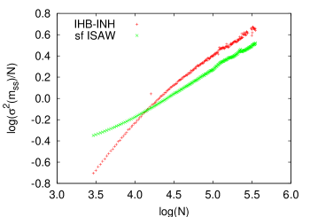
Figure 11: The maximum of fluctuations for the transition between the globule and crystalline phases for two models: semi-flexible ISAW (a) and the IHB–INH (b) models. (The first curve (a) is shifted to show them next to each other.)

However, by being conservative with taking into account the corrections to scaling for the largest lengths we have estimated the exponent to be $0.4(2)$. Now, this exponent is expected to be $\alpha\phi$ where $\alpha$ is the specific heat exponent of the thermodynamic limit transition and $\phi$ is the crossover exponent. Additionally it is usually expected that $2-\alpha=1/\phi$ so we have $\alpha=0.6(2)$ and $\phi=0.7(1)$.

5 Semi-flexible INH model ($\beta_{hb}=0$)

Given that we have investigated the effect of stiffness on the IHB model and previously [14] considered the IHB–INH model [14] it was desirable to consider the effect of stiffness on the INH model for completeness.

When $\beta_{ss}=0$ the INH model behaves exactly as the ISAW with a single collapse transition from the extended phase at high temperatures to the globular collapsed phase at low temperatures. While it is more difficult to detect the $\theta$ point in two dimensions since the specific heat exponent $\alpha<0$ it signature can still be seen in the specific heat data. We have determined a finite size phase boundary $\beta_{nh}^{(c)}(\beta_{ss};n=128)$ that can be seen in Figure 12. We immediately see that while the INH model behaves similarly to the ISAW model the addition of stiffness does not produce the same effect. At most one phase transition is found for any positive or negative stiffness energy.

On both lattices we therefore have found that the addition of negative stiffness (effectively encouraging bends) to the interacting non-hydrogen-bond model leaves the single phase transition from a swollen phase at high temperatures to a globular phase at low temperatures unchanged. This can be simply understood by noting that most of the non-hydrogen-bond contacts occur between bends in the walk anyway. The transition temperature goes to zero as the stiffness energy goes to negative infinity.

When favouring straight segments, so that $\varepsilon_{ss}$ and $\beta_{ss}$ are positive, then when any transition occurs it is again of a similar type as the fully-flexible model (that is $\theta$-point-like). However, at least for $\lambda=\varepsilon_{ss}/\varepsilon_{nh}$ large enough no phase transition occurs on lowering the temperature.

A similar argument to the one in Section 3 seems to hold: non-hydrogen-bond contacts do not occur between stiffness sites which are favoured by large positive values of $\varepsilon_{ss}$. We note that the zero temperature states are pathological and there exits zero temperature phases transitions (rod-coil and rod-globule). Nevertheless it seems that the change in the zero-temperature state on varying the parameters still accords with the position of the finite temperature swollen-globule phase boundary. At zero temperatures the ground state for $\lambda>2$ is a walk consisting only of straight segments with energy $-n\varepsilon_{ss}$. For $0<\lambda<2$ the ground state consists of long zig-zag paths with each ‘zig’ and each ‘zag’ being made up of two steps (in this way each straight segment is always adjacent to two bends) next to each other which have one non-hydrogen bond per step and one stiffness parameter per two steps: the energy of this state is $-n\varepsilon_{hb}-\frac{n}{2}\varepsilon_{ss}$. These two states cross energies at $\lambda=2$: this seems to explain the asymptote of the phase boundary in Figure 12 for large positive $\varepsilon_{ss}$.

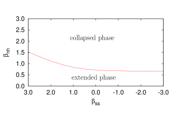
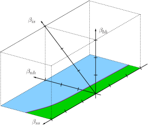
Figure 12: Plot of the finite size phase boundary for the semi-flexible INH model on the square lattice (top). The plane of the parameters of the semi-flexible INH model in the more general three parameter space: the two phases are denoted by a light (blue) shading for the globular phase and a mid-density(green) shading for the extended swollen polymer phase. (bottom)

6 Conclusions

We have investigated the effect of increasing stiffness and also enhancing bends on the lattice model of hydrogen-bonded polymers. We have found that in both cases if there is a phase transition it is unchanged from the fully-flexible model: namely a first order phase transitions occurs in both two and three dimensions. We also argue that if bending is sufficiently enhanced no phase transition occurs at all. This is in contrast to the effect of adding stiffness to the canonical model of self-interacting polymers where adding stiffness results in three phases: a high temperature excluded-volume dominated “swollen” phase, a liquid-like globule phase and an anisotropic solid-like polymer crystal phase. We have investigated this semi-flexible ISAW problem in two dimensions and shown that these three phases exist as they had previously been shown to exist in three dimensions. We have investigated the globule-crystal transition on the square lattice more closely and found that unlike three dimensions where it is first order but like another recently studied model, extending the hydrogen bonding model by the addition of non-hydrogen bond interactions, the transition is second order with specific heat exponent $\alpha=0.6(2)$.

Putting together all the information at hand it is likely that in the three-dimensional phase space of hydrogen-bond, non-hydrogen-bond nearest neighbour interactions and stiffness only the three phases already studied occur. In Figure 13 all the phase boundaries found when the energies are all positive are illustrated. One can the infer that for $\beta_{hb}$ and $\beta_{nh}$ small no matter what the value of $\beta_{ss}$ the extended phase exists. Also, one can infer that for large $\beta_{nh}$ the globular phase exists and for large $\beta_{nh}$ the crystal phase exists. In this way the partial results in the literature can now be understood.

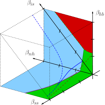
Figure 13: The phase boundaries found in the full three-dimensional phase space. We conjecture that only three phases occur in this larger space. we have illustrated the phases in the planes $\beta_{hb}=0$ and $\beta_{ss}=0$ in the quadrant where all the energies are positive: the three phases are denoted by a light (blue) shading for the globular phase, a mid-density (green) shading for the extended swollen polymer phase and a dark (red) shading for the crystalline phase.

References

- [1] Flory P, 1971 Principles of Polymers Chemistry (Ithaca, NY: Cornell University Press)
- [2] de Gennes P-G, 1979 Scaling Concept in Polymer Physics (Ithaca, NY: Cornell University Press)
- [3] Vanderzande C, 1998 Lattice Models of Polymers (Cambridge, UK: Cambridge University Press)
- [4] des Cloizeaux J and Janninck G, 1990 Polymers in Solutions: Their Modelling and Structure (Oxford, UK: Oxford University Press)
- [5] Prellberg T and Owczarek A L, 1994 J. Phys. A: Math. Gen. 27 1811
- [6] Bastolla U and Grassberger P, 1997 J. Stat. Phys. 89 1061
- [7] Vogel T, Bachmann M and Janke W, 2007 Phys. Rev. E 76 061803
- [8] Doye J P K, Sear R P and Frenkel D, 1997 J. Chem. Phys. 108 2134
- [9] Jacobsen J L and Kondev J, 2004 Phys. Rev. Lett. 92 210601
- [10] Pauling L and Corey R B, 1951 PNAS 37 235, 251, 272, 729
- [11] Bascle J, Garel T and Orland H, 1993 J. Phys. II France 3 245
- [12] Foster D P and Seno F, 2001 J. Phys. A: Math. Gen. 34 9939
- [13] Krawczyk J, Owczarek A L, Prellberg T and Rechnitzer A, 2007 Phys. Rev. E 76 51904
- [14] Krawczyk J, Owczarek A L, and Prellberg T, 2007 J. Stat. Mech. P09016
- [15] Prellberg T and Krawczyk J, 2004 Phys. Rev. Lett. 92 120602