Using polarized maser to detect high-frequency relic gravitational waves

A GHz maser beam with Gaussian-type distribution passing through a homogenous static magnetic field can be used to detect gravitational waves (GWs) with the same frequency. The presence of GWs will perturb the electromagnetic (EM) fields, giving rise to perturbed photon fluxes (PPFs). After being reflected by a fractal membrane, the perturbed photons suffer little decay and can be measured by a microwave receiver. This idea has been explored to certain extent as a method for very high frequency gravitational waves. In this paper, we examine and develop this method more extensively, and confront the possible detection with the predicted signal of relic gravitational waves (RGWs). A maser beam with high linear polarization is used to reduce the background photon fluxes (BPFs) in the detecting direction as the main noise. As a key factor of applicability of this method, we give a preliminary estimation of the sensitivity of a sample detector limited by thermal noise using currently common technology. The minimal detectable amplitude of GWs is found to be $h_{\rm{min}}\sim 10^{-30}$. Comparing with the known spectrum of the RGWs in the accelerating universe for $\beta=-1.9$, there is still roughly a gap of $4\sim 5$ orders. However, possible improvements on the detector can further narrow down the gap and make it a feasible method to detect high frequency RGWs.

PACS numbers: 04.30.Nk, 04.80.Nn, 95.55.Ym, 98.80.-k

I. INTRODUCTION

Although there has been some indirect evidence of GWs radiation from the binary pulsar B1913+16 [1], so far GWs have not been directly detected yet. Currently, a number of detectors have been running or under construction. These detectors use various methods including: (1) the conventional method of cryogenic resonant bar [2] aiming at a frequency around $10^{3}$ Hz; (2) the method of ground-based laser interferometers, such as LIGO [3], VIRGO [4], GEO [5], TAMA [6], and AIGO [7], applying for a frequency range $10\sim 10^{3}$ Hz, and the space-based laser interferometers LISA [8] under planning for a lower frequency range $(10^{-3},10^{-1})$ Hz; (3) the detections of cosmic microwave background radiation (CMB) polarization of “magnetic” type, or the temperature-“electric” cross-correlation [9], which would also give direct evidence of GWs [10] for very low frequencies around $(10^{-18},10^{-16})$ Hz. Besides, there have also been attempts, based on various techniques, to detect GWs of very high frequencies from MHz to GHz, such as the waveguide detector to measure the change of polarizations of EM waves [11, 12], the two coupled microwave cavities to measure small harmonic displacements [13], and laser interferometers [14], etc.

There is another method of detection for high frequency gravitational waves (HFGWs), which employs a a maser beam passing through a strong static magnetic field [15, 16, 17], and uses a microwave receiver in combination with a fractal membrane [18, 19]. The maser beam can be chosen to a free electron maser [20, 21] with a great output power $\sim 2$ kW, whose frequency $\sim 4.5$ GHz is the one that the fractal membrane operates effectively [22, 23, 24]. In the presence of GWs, the background EM fields will be perturbed, giving rise to additional photon fluxes in various directions. In the previous studies by Li et al [17, 19], an ordinary maser beam is used, in which case the BPFs always exist and tend to mix up with the PPFs, forming a kind of noise. Moreover, in order to assess the method as a potential way to detect GWs, the sensitivity of the detection predicted by this method has to be estimated, and a comparison with the predicted spectrum of RGWs [25]-[29] is still needed. In this paper, we improve the method by using a linearly polarized maser beam, so that the BPFs in the detecting direction can be suppressed effectively.

Generally speaking, HFGWs in GHz band are not generated by usual astrophysical processes, such as explosions of asymmetric supernovas, rotations of binary stars around each other, coalescing and merging of binary neutron stars or black holes, and collapse of stars [30, 31, 32]. There could be a thermal background of gravitational waves, which consists of gravitons in thermal equilibrium [33, 34]. But, it will be examined that, if the inflationary expansion did occur in the early universe, the possible thermal GWs will be negligibly small. As is known, RGWs generated by the inflation have a spectrum stretching over a whole range of $(10^{-18},10^{11})$ Hz. In particular, it has a considerable amount of power around the very high frequency range $\sim 4.5$ GHz. Thus it can serve as the main target of detection using the maser beam. We shall estimate qualitatively the sensitivity of detection of a sample detector, and make a comparison with the known analytic spectrum of RGWs [27, 28, 29], which has not been made before.

The organization of the paper is as follows. In Section II, we describe a setup of maser-beam GW detection. In Section III we study the PPFs density caused by the incident GWs propagating along various directions, and estimate the number of the perturbed photons per second passing through a receiving surface. Section IV is devoted to a preliminary analysis of the sensitivity of the detector limited by the thermal noise, and to the discussion of the feasibility of detecting the RGWs in the accelerating universe. In Section V, a summary is given. The Appendix gives a detailed calculation of the PPFs density generated by the incident GWs along the positive $z$-direction.

II. THE SETUP OF THE DETECTOR

The idea of the maser beam gravitational wave detector is based on the property that the maser beam in the presence of a homogeneous static magnetic field will be perturbed when GWs pass by [16, 19]. In particular, under the resonance condition that the frequency of GWs equals that of the maser beam ($\nu_{g}=\nu_{e}$), additional PPFs will be generated and serve as a signal of GWs to be detected. As can be seen later, the magnitude of the PPFs is proportional to the amplitude of GWs and to the static magnetic field as well. Fig.1 shows the geometric configuration of the setup for the detector. The maser beam of frequency $\nu_{e}\sim 4.5$ GHz travels along the positive $z$-direction and passes through the static magnetic field $\sim$ 3 Tesla pointing to the positive $y$-direction. The PPF density (photons per unit area per unit time) in the $x$-direction, $n_{x}^{(1)}$, after being totally reflected by a fractal membrane [22, 23, 24], will keep its strength constant within a distance of about $1$ meter. The reflected PPF density $n_{x}^{(1)^{\prime}}$ will be received by a microwave receiver as a signal of GWs. As a typical pattern, some of the generated PPFs will travel around the maser beam [16], forming a circular flux, which is shown in Fig.2.

Although the maser beam is set to propagate along the positive $z$-direction overwhelmingly, there is always a leakage flux of photons along the radial direction (normal to the $z$-direction). These leaking photons will mix up with the perturbed photons and form a noise for detection. Since we have chosen to detect the PPFs in the $x$-direction, we should try to eliminate the BPFs in the $x$-direction. This can be achieved by using a linearly polarized maser beam. Maser beams in the GHz band have been generated under laboratory conditions [20, 21]. In our setup of the detector, we make use of a maser beam with transverse electric mode ($\mathrm{TEM}_{00}$), whose strength has a Gaussian-type distribution [35]:

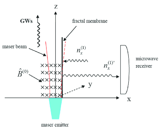
Figure 1: The sketch map of the setup of detection. The maser beam is propagating along the positive $z$-direction, and the static magnetic field points to the positive $y$-direction as represented by the furcations. The envelope of the maser beam is sketched as the hyperbola. The fractal membrane is placed in the $y-z$ plane near the maser beam, facing to the right. The portion of the PPFs along the negative $x$-direction is reflected by the fractal membrane. The reflected PPF density $n_{x}^{(1)^{\prime}}$ goes along the positive $x$-direction and keep its strength constant within 1 meter. The microwave receiver is placed on the right, facing to the left, and catching the outgoing perturbed photons as the signal.

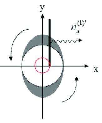
Figure 2: A sketch map of the circular perturbed photon flux. The inner circle stands for the maser beam. The dark areas stand for the perturbed photon flux in the circular direction, where the thicker region means a larger flux. The membrane is placed near the Gaussian beam and the flux is reflected back into the positive $x$-direction.

$$\psi({\bf x},t)=\frac{\psi_{0}}{\sqrt{1+(z/f)^{2}}}\exp(-\frac{r^{2}}{W^{2}})\exp\left\{i[(k_{e}z-\omega_{e}t)-\tan^{-1}{\frac{z}{f}}+\frac{k_{e}r^{2}}{2R}+\delta]\right\},$$ (1)

where $\psi_{0}$ is the amplitude on the plane $z=0$, $r=\sqrt{x^{2}+y^{2}}$ is the radial distance, $W=W_{0}[1+(z/f)^{2}]^{1/2}$ with $W_{0}$ being the radius of the beam on the plane $z=0$, $f=W_{0}^{2}k_{e}/2$, $k_{e}=2\pi/\lambda_{e}$ is the wavenumber, $\omega_{e}$ is the angular frequency, $R=z+f^{2}/z$ is the curvature radius of the wave fronts of the beam at $z$, and $\delta$ is an arbitrary phase factor. Furthermore, the maser beam is linearly polarized along the $x$-direction, namely, the electric field in the maser beam is given by

$$\tilde{E}_{x}^{(0)}({\bf x},t)=\psi({\bf x},t),\ \qquad\tilde{E}_{y}^{(0)}=\tilde{E}_{z}^{(0)}=0,$$ (2)

where the tilde “$\sim$” and the superscript $``(0)$” stand for the time-dependent and the background EM fields, respectively. Since the maser beam emitted from the emitter is in the region $z\geq 0$. the static magnetic field is chosen to localize in the region $z\geq 0$,

$$\hat{B}^{(0)}=\left\{\begin{array}[]{cc}\hat{B}_{y}^{(0)}&(0\leq z\leq l),\\ 0&\ \ \qquad(z<0\ \ {\mathrm{or}}\ \ z>l),\end{array}\right.$$ (5)

where the caret “$\wedge$” denotes the static magnetic field, and $l$ is the dimension of the static magnetic field in the $z$-direction.

In absence of GWs, the components of the average BPF density ($m^{-2}s^{-1}$) are given as follows,

$$n_{x}^{(0)} = 0,$$ (6)

$$n_{y}^{(0)} = -\frac{1}{\mu_{0}\hbar\omega_{e}}\langle\tilde{E}_{x}^{(0)}\tilde{B}_{z}^{(0)}\rangle$$ (7)

$$= \frac{\psi_{0}^{2}k_{e}y}{2\mu_{0}\hbar\omega_{e}^{2}[1+(z/f)^{2}](z+f^{2}/z)}\exp{(-\frac{2\,r^{2}}{W^{2}})},$$

$$n_{z}^{(0)} = \frac{1}{\mu_{0}\hbar\omega_{e}}\langle\tilde{E}_{x}^{(0)}\tilde{B}_{y}^{(0)}\rangle$$ (8)

$$= \frac{\psi_{0}^{2}}{2\mu_{0}\hbar\omega_{e}^{2}[1+(z/f)^{2}]}\left[k_{e}+\frac{k_{e}r^{2}(f^{2}-z^{2})}{2(f^{2}+z^{2})^{2}}-\frac{f}{f^{2}+z^{2}}\right]\exp{(-\frac{2\,r^{2}}{W^{2}})},$$

where “$\langle\rangle$” means the average over a time scale much longer than $1/\nu_{e}$. Note that, since the maser has been chosen to be linearly polarized in $x$-direction, the $x$-component of the BPF density, $n_{x}^{(0)}$ as a noise, is vanishing. This feature is an advantage over that using an unpolarized beam [19]. Of course, in actual situation, the maser beam can not be polarized completely. Then, Eq.(6) is not valid strictly, and it always exits the residual BPF density $n_{x}^{(0)}$. Just like the components $n_{y}^{(0)}$ and $n_{z}^{(0)}$, $n_{x}^{(0)}$ will decay by a factor $e^{-\frac{2r^{2}}{W^{2}}}$, moreover, the fractal membrane only reflects the PPF not the BPF [19]. However, after reflected by the fractal membrane, $n_{x}^{(1)}$ will not decay within 1 meter. Then, at a large radial distance $r$ from the beam, $n_{x}^{(0)}$ can be negligible compared with $n_{x}^{(1)}$. We will discuss about this problem in more details in Sec III.

A. GWs along positive $z$-direction

The situation we are interested in is when GWs are present. Consider a beam of circularly polarized monochromatic plane GWs propagating along the positive $z$-axis. The metric can be written as

$$g_{\mu\nu}=\eta_{\mu\nu}+h_{\mu\nu},$$ (9)

where $\eta_{\mu\nu}$ is Minkowsky metric, and $h_{\mu\nu}$ stands for GWs with $|h_{\mu\nu}|\ll 1$. In TT (transverse-traceless) gauge, $h_{\mu\nu}$ has only two independent components: $h_{11}=-h_{22}\equiv h_{\oplus}$, and $h_{12}=h_{21}\equiv h_{\otimes}$, where

$$h_{\oplus}=A_{\oplus}\exp{[i(k_{g}z-\omega_{g}t)]},$$

$$h_{\otimes}=iA_{\otimes}\exp{[i(k_{g}z-\omega_{g}t)]}.$$ (10)

In a curved spacetime, the Maxwell’s equations in vacuum are [36, 37]

$$(\sqrt{g}\,g^{\mu\alpha}g^{\nu\beta}F_{\alpha\beta})_{,\,\nu}=0,$$ (11)

$$F_{\mu\nu,\,\sigma}+F_{\nu\sigma,\,\mu}+F_{\sigma\mu,\,\nu}=0,$$ (12)

where $F_{\mu\nu}$ is the EM field tensor, $g\equiv-{\mathrm{det}}(g_{\mu\nu})$, and the comma means the ordinary derivative. Since the EM field will be perturbed by GWs, we decompose the total EM tensor into two parts:

$$F_{\mu\nu}=F_{\mu\nu}^{(0)}+F_{\mu\nu}^{(1)},$$ (13)

where $F_{\mu\nu}^{(0)}$ represents the background fields, and $F_{\mu\nu}^{(1)}$ the perturbed fields caused by GWs. Explicitly,

$$F^{(0)}_{\mu\nu}=\frac{1}{c}\left(\begin{array}[]{cccc}0&-\tilde{E}_{x}^{(0)}&0&0\\ \tilde{E}_{x}^{(0)}&0&c\tilde{B}_{z}^{(0)}&-c(\hat{B}_{y}^{(0)}+\tilde{B}_{y}^{(0)})\\ 0&-c\tilde{B}_{z}^{(0)}&0&c\tilde{B}_{x}^{(0)}\\ 0&c(\hat{B}_{y}^{(0)}+\tilde{B}_{y}^{(0)})&-c\tilde{B}_{x}^{(0)}&0\end{array}\right),$$ (18)

$$F^{(1)}_{\mu\nu}=\frac{1}{c}\left(\begin{array}[]{cccc}0&-\tilde{E}_{x}^{(1)}&-\tilde{E}_{y}^{(1)}&-\tilde{E}_{z}^{(1)}\\ \tilde{E}_{x}^{(1)}&0&c\tilde{B}_{z}^{(1)}&-c\tilde{B}_{y}^{(1)}\\ \tilde{E}_{y}^{(1)}&-c\tilde{B}_{z}^{(1)}&0&c\tilde{B}_{x}^{(1)}\\ \tilde{E}_{z}^{(1)}&c\tilde{B}_{y}^{(1)}&-c\tilde{B}_{x}^{(1)}&0\end{array}\right).$$ (23)

Since $|h_{\mu\nu}|\ll 1$, $F_{\mu\nu}^{(1)}$ is also small and will be evaluated up to the first order of $|h_{\mu\nu}|$. As will be seen, each component $F_{\mu\nu}^{(1)}$ receives two parts of contributions: one comes from the interaction between the static magnetic field and the GWs, $\propto|h_{\mu\nu}|\hat{B}^{(0)}$, the other comes from the interaction between the maser beam and the GWs, $\propto|h_{\mu\nu}|\tilde{B}^{(0)}$ [38, 39, 15]. In our designing of the detection, the static magnetic field is chosen to be so large that $\tilde{B}^{(0)}/\hat{B}^{(0)}\sim 10^{-5}$ [19]. Therefore, in $F_{\mu\nu}^{(1)}$ we only keep the contribution $\propto|h_{\mu\nu}|\hat{B}^{(0)}$. The maser beam just provides the resonance condition to generate the PPFs, i.e., the detector only respond to the GWs with the same frequency as the maser beam. By solving the Maxwell’s equations (11), one obtains the perturbed EM fields and the PPFs. The detailed calculation of $n_{x}^{(1)}$ is given in Appendix. The resulting expressions of the PPFs density $n_{x}^{(1)}$ in all three regions are given by

Region I $(z\leq 0)$.

$$n_{x}^{(1)}=0;$$ (24)

Region II $(0\leq z\leq l)$,

$$n_{x}^{(1)}=-\frac{A_{\otimes}\hat{B}_{y}^{(0)}\psi_{0}y}{2\mu_{0}\hbar\omega_{e}[1+(z/f)^{2}]^{1/2}}\left\{\frac{k_{g}z}{2(z+f^{2}/z)}\sin{\Phi}\right.$$

$$\qquad\quad\left.+\frac{z}{W_{0}^{2}[1+(z/f)^{2}]}\cos{\Phi}+\frac{1}{2(z+f^{2}/z)}\sin{(k_{g}z)}\sin{\left(k_{g}z+\Phi\right)}\right.$$

$$\qquad\quad\left.+\frac{1}{k_{g}W_{0}^{2}[1+(z/f)^{2}]}\sin{(k_{g}z)}\cos{\left(k_{g}z+\Phi\right)}\right\}\exp{\left(-\frac{r^{2}}{W^{2}}\right)};$$ (25)

Region III $(z\geq l)$,

$$n_{x}^{(1)}=-\frac{A_{\otimes}\hat{B}_{y}^{(0)}\psi_{0}yl}{2\mu_{0}\hbar\omega_{e}[1+(z/f)^{2}]^{1/2}}\left\{\frac{k_{g}}{2(z+f^{2}/z)}\sin{\Phi}\right.$$

$$\qquad\quad\left.+\frac{1}{W_{0}^{2}[1+(z/f)^{2}]}\cos{\Phi}\right\}\exp{\left(-\frac{r^{2}}{W^{2}}\right)},$$ (26)

where $\mu_{0}$ is the permeability in vacuum, and

$$\Phi\equiv\frac{k_{g}r^{2}}{2R}-\arctan{(\frac{z}{f})}.$$ (27)

The phase $\delta=\pi/2$ has been taken for concreteness. As Eqs.(Using polarized maser to detect high-frequency relic gravitational waves) and (Using polarized maser to detect high-frequency relic gravitational waves) show, $n_{x}^{(1)}$ is only produced by the GWs of $\otimes$-polarization mode, and is proportional to the static magnetic field $\hat{B}_{y}^{(0)}$ and the maximal amplitude $\psi_{0}$ of the maser beam. Since $|n_{x}^{(1)}|$ contains a decaying factor $e^{-r^{2}/W^{2}}$, it decreases radially for larger $r$. To visualize the dependence of $n_{x}^{(1)}$ on spatial variables, we plot it as a function of $(y,z)$ on the plane $x=0.05$ m in Fig.3, and as a function of $(x,y)$ on the plane $z=0.4$ m in Fig.4.

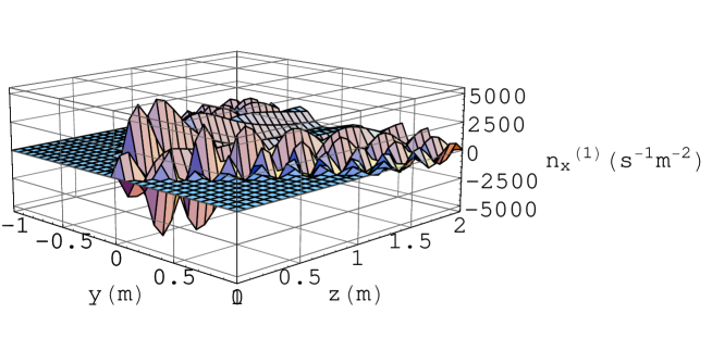
Figure 3: $n_{x}^{(1)}$ as a function of $(y,z)$ on the plane $x=0.05$ m. The parameters are taken as $A_{\otimes}\sim 10^{-30}$, $\psi_{0}=1.8\times 10^{4}$  V m^-1, $W_{0}=0.05$ m,  $\hat{B}_{y}^{(0)}=3$ T, and $l=0.4\,$m for demonstration.

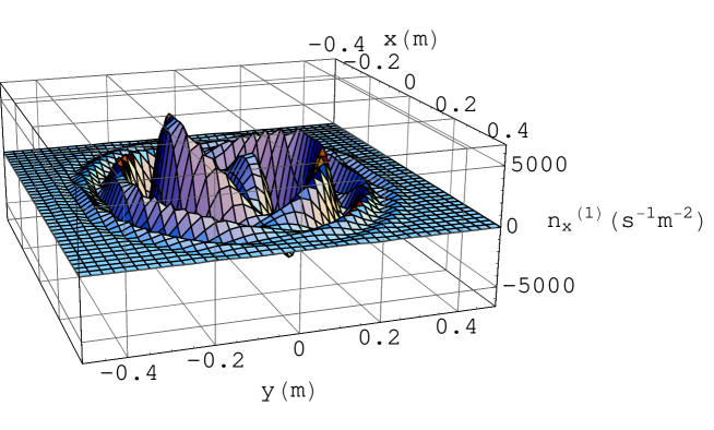
Figure 4: $n_{x}^{(1)}$ as a function of $(x,y)$ on the plane $z=0.4$ m. The parameters are taken the same as in Fig.3.

B. GWs along some other directions

The above is for the incident GWs along the positive $z$-axis. In this section, we give the results of incident GWs propagating along other directions, while the setup of the detector is the same as in Section II.

(1) The incident GWs propagating along the negative $z$-direction. The relevant results are the following:

Region II ($0\leq z\leq l$),

$$n_{x}^{(1)}=\frac{A_{\otimes}\hat{B}_{y}^{(0)}\psi_{0}y}{2\mu_{0}\hbar\omega_{e}[1+(z/f)^{2}]^{1/2}}\left\{\frac{k_{g}(z-l)}{2(z+f^{2}/z)}\sin{\left(2k_{g}z+\Phi\right)}\right.$$

$$\qquad\quad+\frac{(z-l)}{W_{0}^{2}[1+(z/f)^{2}]}\cos{\left(2k_{g}z+\Phi\right)}\left.+\frac{1}{2(z+f^{2}/z)}\sin{(k_{g}z)}\sin{\left(k_{g}z+\Phi\right)}\right.$$

$$\qquad\quad\left.+\frac{1}{k_{g}W_{0}^{2}[1+(z/f)^{2}]}\sin{(k_{g}z)}\cos{\left(k_{g}z+\Phi\right)}\right\}\exp{\left(-\frac{r^{2}}{W^{2}}\right)};$$ (28)

Region III ($z>l$),

$$n_{x}^{(1)}=0.$$ (29)

Since the maser emitter lies in Region I ($z<0$), so it is not interesting for detection.

(2) The incident GWs propagating along the positive $x$-direction. The static magnetic field $\hat{B}^{(0)}_{y}$ is taken to be localized in the region $-l_{1}\leq x\leq l_{2}$ in the $x$-direction. One obtains

$$n_{x}^{(1)}=\frac{A_{\otimes}\hat{B}_{y}^{(0)}\psi_{0}y}{2\mu_{0}\hbar\omega_{e}[1+(z/f)^{2}]^{1/2}}\left\{\frac{k_{g}(x+{l_{1}})}{2(z+f^{2}/z)}\sin{[k_{g}(z-x)+\Phi]}\right.$$

$$\qquad\quad+\frac{x+l_{1}}{W_{0}^{2}[1+(z/f)^{2}]}\cos{[k_{g}(z-x)+\Phi]}\left.+\frac{1}{2(z+f^{2}/z)}\sin{(k_{g}x)}\sin{\left(k_{g}z+\Phi\right)}\right.$$

$$\qquad\quad\left.+\frac{1}{k_{g}W_{0}^{2}[1+(z/f)^{2}]}\sin{(k_{g}x)}\cos{\left(k_{g}z+\Phi\right)}\right\}\exp{\left(-\frac{r^{2}}{W^{2}}\right)}$$ (30)

for the region $-l_{1}\leq x\leq l_{2}$.

(3) The incident GWs propagating along the negative $x$-direction. With the static magnetic field as in (2), one has

$$n_{x}^{(1)}=-\frac{A_{\otimes}\hat{B}_{y}^{(0)}\psi_{0}y}{2\mu_{0}\hbar\omega_{e}[1+(z/f)^{2}]^{1/2}}\left\{\frac{k_{g}(x-l_{2})}{2(z+f^{2}/z)}\sin{[k_{g}(z+x)+\Phi]}\right.$$

$$\qquad\quad+\frac{x-l_{2}}{W_{0}^{2}[1+(z/f)^{2}]}\cos{[k_{g}(z+x)+\Phi]}\left.+\frac{1}{2(z+f^{2}/z)}\sin{(k_{g}x)}\sin{\left(k_{g}z+\Phi\right)}\right.$$

$$\qquad\quad\left.+\frac{1}{k_{g}W_{0}^{2}[1+(z/f)^{2}]}\sin{(k_{g}x)}\cos{\left(k_{g}z+\Phi\right)}\right\}\exp{\left(-\frac{r^{2}}{W^{2}}\right)},$$ (31)

which is similar to Eq.(Using polarized maser to detect high-frequency relic gravitational waves).

(4) The incident GWs propagating along the positive or negative $y$-direction. One finds that $\tilde{E}_{y}^{(1)}=0$, leading to

$$n_{x}^{(1)}=0.$$ (32)

The above results show that, for the given setup, the detector responses differently to the incident GWs from different directions. In the following it will be seen that the detector responses most effectively to the GWs in the $z$-direction. In general, RGWs is of stochastic nature and come from various directions. In this case, a reduction factor will be introduced as shown later.

C. Numerical calculations for PPFs

In order to examine the dependence of perturbed photons on the directions in which GWs propagate, let us estimate numerically the perturbed photons per unit time received by the microwave receiver for the above cases of the incident GWs. For concreteness, we adopt the following parameters of the detector that can be realized in the laboratory:

1) $P=2$ kW, the power of the maser beam, corresponding to $\psi_{0}=1.8\times 10^{4}$ Vm^-1 for the spot radius $W_{0}=0.05\,$m [20, 21].

2) $\hat{B}_{y}^{(0)}=3$ Tesla, the strength of the background static magnetic field [40].

3) $l=0.4\,$m, the width of the static magnetic field in $z$-direction.

4) $l^{\prime}=l_{1}+l_{2}=0.4\,$m, the width of the static magnetic field in $x$-direction.

5) $\nu_{e}\simeq 4.5$ GHz, the frequency of the maser beam in the microwave band [20, 21].

The number of perturbed photons in the $x$-direction per second passing through a surface $\Delta s$ on the plane $x=0.05$m is given by:

$$N_{x}^{(1)}=\int\limits_{\Delta s}n_{x}^{(1)}|_{x=0.05}\ {\mathrm{d}}y{\mathrm{d}}z.$$ (33)

Here the integrand is taken to be the negative portion of $n_{x}^{(1)}<0$, which is reflected by the membrane back to the positive $x$-direction. For comparison, we choose $\Delta s\simeq 8\times 10^{-2}\,$m² ($0\leq y\leq 0.2\,$m, $0\leq z\leq 0.4\,$m) to receive more photons with a limited size. For concreteness, $A_{\otimes}\sim 10^{-30}$ is taken. The resulting $N_{x}^{(1)}$ is shown in Table 1. We see that the magnitude of $N_{x}^{(1)}$ generated by the incident GWs along the positive $z$-direction and the positive $x$-direction has the same order, which is larger than that for other cases. Note, for the case of GWs along $y$-direction, $N_{x}^{(1)}$ is nearly vanishing.

Using the parameters given above, if we choose the maser beam to have a polarization degree is $\sim 98\%$, corresponding to a ratio of unpolarized/polarized electric field components $\tilde{E}_{y}^{(0)}/\tilde{E}_{x}^{(0)}\sim 0.1$, our computation shows that the ratio of the number of background/perturbed photons over the area $\Delta s$ per second will be

$$N_{x}^{(0)}/N_{x}^{(1)}\sim 10^{-7}$$ (34)

at $x\simeq 1\,m$ . So, if the microwave receiver is put at $\sim 1$ meter away from the fractal membrane, the influence of the background photon flux will be effectively negligible. A higher polarization of the maser beam is always wanted to suppress the BPF.

Table 1: The number of photons per second passing through $\Delta s$, $N_{x}^{(1)}$, for GWs from various directions.

Direction of GWs	$N_{x}^{(1)}(s^{-1})$
$+z$	$\sim 1\times 10^{2}$
$-z$	$\sim 5.4\times 10$
$+x$	$\sim 1.2\times 10^{2}$
$-x$	$\sim 3.4$
$\pm y$	$\sim 0$

Remember that the phase $\delta=\pi/2$ has been taken in the above for simplicity. However, in general, $N_{x}^{(1)}$ would depend on the phase factor $\delta$. Fig.5 (a),(b),(c) and (d) give $N_{x}^{(1)}$ as a function of $\delta$ for the incident GWs along $+z,-z,+x$ and $-x$, respectively. Fig.5 shows that the changes of $N_{x}^{(1)}$ with $\delta$ is small, and the error for various values of $\delta$ is less than $4\%$. Thus, in the following, we assume that $N_{x}^{(1)}$ is independent of the phase factor $\delta$.

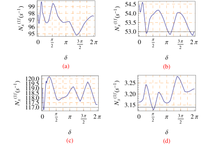
Figure 5: The small fluctuation of $N_{x}^{(1)}$ with variable $\delta$. (a),(b),(c) and (d) give the cases of the incident GWs along $+z,-z,+x$ and $-x$, respectively.

IV. THE DETECTION FOR RGWs

In this section, we estimate the sensitivity of the detector, and analyze the feasibility of detecting the RGWs using this method.

A. Implementation of the experiment

One certainly expects to have a number of problems in the actual implementation of such kind of detection. There could be various sorts of noises for this detector, such as thermal noise, external EM noise, seismic noise, and shot noise in the maser beam, etc. The seismic noise is one of major obstacles for the common laser interferometer detectors. However, this kind of noise usually has a frequency much lower than GHz band and will not generate additional perturbed photons, so it will not affect our detection essentially. Still, an isolating system may be employed. For instance, the detector system may be put on a suspended framework to absorb seismic vibrations. As for the shot noise in the maser beam, it can be suppressed by stabilizing the frequency and the amplitude of the maser beam.

Among all these kinds of noises, the external EM noise would be a real problem for our detection. For example, the CMB at $T\sim 2.7$ K yields a photon flux density $n\sim 10^{4}$ $cm^{-2}s^{-1}$ around the frequency $\nu\sim 4.5$ GHz with a width $\Delta\nu\simeq 10$ KHz (the frequency width of the maser) in any direction. The energy flux of CMB photons would overwhelm that of the perturbed photons, since the average PPF density $\bar{n}_{x}^{(1)}\sim 0.6$ $cm^{-2}s^{-1}$ as from Table 1 where we have assumed $A_{\otimes}\sim 10^{-30}$. To solve the problem, we propose to employ a Faraday cage, which shields the detecting device from the external EM noise. The outer shell of the cage may be made of some conducting metal so that the external EM waves will not entering the cage. The inner surface of the cage should be made of some kind of material that effectively absorbs noise photons within the cage. So the CMB photons and other EM noise inside the cage can be eliminated. In designing the Faraday cage, we should excavate a little hole on the cage and the hole should be sealed by a one-way membrane with a total transmittance around $4.5$ GHz, so that the maser beam can pass through it while the photons can not enter the cage.

Furthermore, to eliminate thermal photons emitted from the detector system and from the inner layer of the cage, one need reduce the temperature of the system. Therefore, a cryogenic technique should be applied so that the detector operates in a low temperature environment. Moreover, a vacuum environment of the system will help for the detection.

B. Sensitivity of detector

For a preliminary analysis, we will focus on the thermal noise in our detection system and estimate its sensitivity limited by thermal noise. The signal power is given by

$$S=\eta|N_{x}^{(1)}|\hbar\omega_{e},$$ (35)

where $\eta$ is the reflectance of the fractal membranes, ranging from $0$ to $1$. With the help of Eq.(33), $N_{x}^{(1)}$ is given by

$$|N_{x}^{(1)}|\simeq\frac{7A_{\otimes}\hat{B}^{(0)}_{y}\psi_{0}}{\mu_{0}\hbar\omega_{e}}\times 10^{-3}\,\,\,s^{-1}.$$ (36)

The input thermal noise (the thermal noise coming into the input part of the receiving system) can be estimated as

$$N_{\rm{in}}=k_{B}TB,$$ (37)

where $k_{B}$ is Boltzmann’s constant, $T$ is the temperature of the thermal noise, and $B$ is the bandwidth of the detector in Hz, which can be estimated as $B\sim\nu_{e}/Q$, where $Q$ is its quality factor. There are additional thermal noises within the receiving system, thus the minimal signal power should satisfy [42]

$$S_{\rm min}=Mf_{0}N_{\rm{in}},$$ (38)

where $M\geq 1$ is the minimal output signal-to-noise, and $f_{0}>1$ is the noise coefficient of the microwave receiver, defined as the ratio of the input signal-to-noise to the output signal-to-noise. Then using Eqs.(36)-(38) and letting $M=1$ yield the minimal detectable dimensionless amplitude,

$$h_{\rm{min}}\simeq\frac{6.4\mu_{0}k_{B}Tf_{0}}{\eta\hat{B}^{(0)}_{y}\psi_{0}Q}\times 10^{11},$$ (39)

where $h_{\rm{min}}\equiv A_{\otimes\,\rm{min}}$. Taking $\psi_{0}=1.8\times 10^{4}$ Vm^-1 and $\hat{B}_{y}^{(0)}=3$ Tesla, $Q=10^{5}$, $T\sim 1$mK [43], $f_{0}\sim 2$, $\eta\sim 99.99\%$ [22, 23, 24], one obtains the sensitivity

$$h_{\rm{min}}\simeq 4\times 10^{-30}.$$ (40)

As said earlier, RGWs come from all directions and form a stochastic background, therefore, in evaluating the sensitivity of the detector, a reduction factor $F$ should be introduced [41]. We can estimate its magnitude as follows. Firstly, we consider the case that the detector responses only to the incident GWs along the positive $z$-direction. By Eqs.(53) and (68) in Appendix,

$$n_{x}^{(1)}\propto\tilde{E}_{\hat{y}}^{(1)}\propto\partial h_{\otimes}(z,t)/\partial z\,\propto k_{z}h_{\otimes}(z,t).$$ (41)

For a beam of incident GWs with a wave vector $\bf k$, one needs to project it along $z$-direction, so that its component $n_{x}^{(1)}\propto k_{z}=k\cos\theta$, where $\theta$ is the angle between $\bf k$ and the positive $z$-direction. Then in this special case the reduction factor $F$ will be estimated as

$$F=\frac{1}{4\pi}\int_{0}^{\frac{\pi}{2}}\cos{\theta}\sin\theta d\theta\int_{0}^{2\pi}d\phi=\frac{1}{4}.$$ (42)

However, this estimate is not complete. In fact, while the detector does not response to the incident RGWs in the $y$-direction, it responses to the incident RGWs in both the $x$- and $z$-directions with the same order of magnitude, as shown in Table 1. For an qualitative estimation, we can take the response of the detector to any incident GWs perpendicular to the $y$-direction to be the same. Consider an arbitrary beam of GWs whose wave vector $\bf k$ forms an angle $\theta$ with the $y$-direction. Projecting the wave vector $\bf k$ on the $x-z$ plane gives rise to a factor $\sim k\sin\theta$. Then, taking the average of $\sin\theta$ over the solid angle $4\pi$ yields

$$F=\frac{1}{4\pi}\int_{0}^{\pi}\sin^{2}{\theta}d\theta\int_{0}^{2\pi}d\phi=\frac{\pi}{4}.$$ (43)

Therefore, we expect that the actual reduction factor $F$ for our detector would be between $1/4$ and $\pi/4$. Multiplying Eq.(36) by $F$, the sensitivity of the detector given by Eq.(40) should be modified as

$$h_{\rm{min}}\simeq(5.1\times 10^{-30}\sim 1.6\times 10^{-29}).$$ (44)

C. Detecting RGWs

What about the detection target, say, the the RGWs in the present accelerating universe [27, 28, 32] around the frequency $\nu_{g}\sim 4.5$ GHz? Now we calculate the root-mean-square (r.m.s.) amplitude of RGWs. In the high frequency limit, the RGWs can be considered approximately as the superposition of plane waves in Eq.(Using polarized maser to detect high-frequency relic gravitational waves). By its nature, RGWs constitute a stochastic background, and the mean value of the field $h_{ij}$ is zero at every instance of time and at every spatial point: $\langle 0|h_{ij}({\mathbf{x}},\tau)|0\rangle=0$. But the variance is not zero [25, 27, 28],

$$\langle h^{2}\rangle\equiv\langle 0|h^{ij}({\mathbf{x}},\tau)\,h_{ij}({\mathbf{x}},\tau)|0\rangle\equiv\int_{0}^{\infty}h^{2}(\nu,\tau)\frac{{\mathrm{d}}\nu}{\nu},$$ (45)

where $h(\nu,\tau)$ is the spectrum of the RGWs, and $\tau$ is the conformal time. Fig.6 gives the spectrum $h(\nu,\tau_{H})$ of the RGWs at the present time $\tau_{H}$ for the cosmological model with the tensor-scalar ratio $r=0.22$, the dark energy $\Omega_{\Lambda}=0.75$, the inflation parameter $\beta=-1.9$, and the reheating parameter $\beta_{s}$ [29]. The quantity $h(\nu,\tau_{H})$ is related to the spectral energy density $\Omega_{g}(\nu)$ often used in literatures[25, 29, 41],

$$\Omega_{g}(\nu)=\frac{\pi^{2}}{3}(\frac{\nu}{\nu_{H}})^{2}h^{2}(\nu,\tau_{H}),$$ (46)

where $\nu_{H}=H_{0}\sim 2\times 10^{-18}$ Hz is the Hubble frequency.

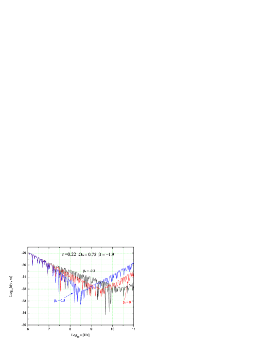
Figure 6: The spectrum of RGWs for the cosmological model with the tensor-scalar ratio $r=0.22$, the dark energy $\Omega_{\Lambda}=0.75$, and the inflation parameter $\beta=-1.9$. The spectrum in GHz band depends sensitively on the reheating parameter $\beta_{s}$ [29].

Due to the resonance condition, the detector only responses to a very narrow frequency band $\Delta\nu\simeq\nu_{g}/Q$ around the central frequency $\nu_{g}$, where $Q$ is the quality factor of the maser beam. Thus, only the modes of frequencies $\nu_{g}\simeq 4.5$ GHz are selected among the incident RGWs. The integration in Eq.(45) is then evaluated as

$$\int_{0}^{\infty}h^{2}(\nu,\tau_{H})\frac{{\mathrm{d}}\nu}{\nu}\simeq h^{2}(\nu_{g},\tau_{H})\frac{\Delta\nu}{\nu_{g}}\simeq h^{2}(\nu_{g},\tau_{H})/Q.$$ (47)

So the r.m.s. amplitude of the RGWs in the band is

$$h_{\rm rms}\equiv\sqrt{\frac{\langle h^{2}\rangle}{2}}\simeq\frac{h(\nu_{g},\tau_{H})}{\sqrt{2Q}},$$ (48)

where $\sqrt{2}$ accounts for the assumption that the $\otimes$- and $\oplus$-polarization modes give equal contribution. Reading from the known spectrum in Fig.6 gives

$$h(\nu_{g},\tau_{H})\sim 8\times 10^{-32}$$ (49)

at $\nu\sim 4.5$ GHz for the reheating model $\beta_{s}=0.5$. The corresponding r.m.s. amplitude is

$$h_{\rm rms}\simeq 1.8\times 10^{-34}.$$ (50)

Comparing Eq.(44) with Eq.(50), one can see that there is approximately a gap of $4\sim 5$ orders of magnitude between the sensitivity of the sample detector and the r.m.s.amplitude of RGWs in the accelerating universe.

As for the possible thermal background of gravitational waves [33, 34], it could have been generated at the very early stage at an energy scale $\sim 10^{19}$ Gev, also described by the Planck spectrum like CMB photons. If there is no inflationary process, the graviton gas would be at $T\sim 1$ K, corresponding to typical frequencies in $\sim 100$ GHz. The amplitude of the spectrum of this thermal GWs would be about $h(\nu)\sim 10^{-32}$ around the frequency of $4.5$ GHz. However, if the inflationary expansion has occurred by some $60$ e-folding, as is supported by WMAP data of CMB anisotropies [44] and others, the thermal GWs would be drastically diluted and its temperature would be reduced to $T\sim 10^{-28}$ K, totally negligible.

D. Possible improvements

Although the sensitivity is still $4\sim 5$ orders short to detect the RGWs, the detector has a large room for improve in several ways. Firstly, note that $h_{\rm min}\propto 1/Q$ by Eq.(39), while $h_{\rm rms}\propto 1/\sqrt{Q}$ by Eq.(48), so the ratio $h_{\rm rms}/h_{\rm min}\propto\sqrt{Q}$. A larger quality factor $Q$ of maser beam will enhance the possibility for detection. This would require a highly monochromatic maser beam. For instance, if $Q$ can be increased from $10^{5}$ to $10^{9}$, the ratio would be enhanced by $\sim 100$ times and the gap will be reduced by $2$ orders. At present, for conventional lasers in the optical frequency band, a quality factor $Q\sim 10^{13}$ has been achieved [45], and for hydrogen maser, the quality factor $Q$ has been reached up to $\sim 10^{9}$ [46, 47, 48]. Secondly, as can be seen from Eq.(39), the sensitivity depends strongly on the temperature $T$ of detector. If it is reduced down to $T\sim 50\mu$K [49], the sensitivity will be improved by a factor $\sim 20$ and the gap will be suppressed to be about 1 order. Thirdly, increasing the strength of the static magnetic field $\hat{B}_{y}^{(0)}$ and the power of the maser will also improve the sensitivity of the detector. Apart from the above possible improvements, enlarging the interaction dimension between the GWs and the static magnetic field will also improve the detection [19]. Putting these possible improvements together, an actual detection will be realistic.

We have extensively studied the maser beam method for detection of GWs $\sim 4.5$ GHz. The experimental setup consists of a maser beam, a strong static magnetic field, a reflecting fractal membrane and a microwave receiver. Moreover, a Faraday cage should be used to prevent the detector from external EM noises. And, to reduce thermal noise, the detector should be place in a low temperature environment. The maser beam is chosen to be linearly polarized, so that the BPF in the detecting direction can be suppressed effectively, and the PPF can be detected as a signal of GWs. We have obtained the analytical expressions for the PPF density $n_{x}^{(1)}$ generated by the incident GWs from various directions.

To examine the feasibility of the detection, we have estimated the sensitivity of the sample detector limited by thermal noise and have confronted it with the RGWs in the accelerating universe as a scientific object. In our preliminary analysis, we found that there was still a gap of about $4\sim 5$ orders between the sensitivity of the detector and the r.m.s. amplitude of the RGWs. However, we have a lot of ways in improving the sensitivity, such as lowering the temperature, increasing the quality factor and the power of maser beam, and enlarging the strength and dimension of the static magnetic field. These improvements will remove the gap, making the method applicable for detecting high frequency RGWs.

However, our analysis on the detection for the RGWs are still tentative, and the conclusions arrived are also preliminary. In particular, the odds is that the detecting PPF as the signal is very small and confronts a number of possible sources of EM noise. A systematical analysis on effectively suppressing these noises is then needed to give a more reliable sensitivity.

Overall, the maser beam method in GHz band or higher is feasible. As a new method to detect GWs, it is complementary to the laser interferometer method working in the low frequency range $(10^{-4}\sim 10^{4})$ Hz. Moreover, from the point of view of experimental constructions, the building of this detection is much less expensive than ordinary interferometer laser methods. Therefore, under these considerations, the GW detection scheme is certainly worthy of further studies and is expected to be implemented in laboratory someday.

ACKNOWLEDGMENTS

Y. Zhang’s work was supported by the CNSF No.10773009, SRFDP, and CAS. F.Y. Li’s work was sopported by CNSF No.10575140 and National Basic Research Program of China under Grant No.2003B716300.

APPENDIX: CALCULATIONS OF $n_{x}^{(1)}$ FOR GWs ALONG DIRECTION OF MASER BEAM

In this appendix, we present the calculations of the PPFs density $n_{x}^{(1)}$ produced by the GWs along the positive $z$-direction. By Eq. (5), the space is divided into three regions: I $(z<0)$, II $(0\leq z\leq l)$, and III $(z>l)$. Firstly, we focus on the region II, where the static magnetic field $\hat{B}_{y}^{(0)}\neq 0$. By Eq.(Using polarized maser to detect high-frequency relic gravitational waves), the expressions of GWs only have two variables $(z,t)$, so will be the perturbed EM fields accordingly. Plugging Eqs. (9) - (23) into Eqs. (11) and (12), and keeping only up to the linear terms of $h_{\mu\nu}$, then after lengthy but easy calculations, one obtains

$$\frac{1}{c^{2}}\tilde{E}^{(1)}_{x,\,t}+\tilde{B}^{(1)}_{y,\,z}=\hat{B}^{(0)}_{y}h_{\oplus,\,z}$$ (51)

$$\tilde{E}^{(1)}_{x,\,z}+\tilde{B}^{(1)}_{y,\,t}=0$$ (52)

$$\frac{1}{c^{2}}\tilde{E}^{(1)}_{y,\,t}-\tilde{B}^{(1)}_{x,\,z}=\hat{B}^{(0)}_{y}h_{\otimes,\,z}$$ (53)

$$\tilde{E}^{(1)}_{y,\,z}-\tilde{B}^{(1)}_{x,\,t}=0,$$ (54)

and

$$\tilde{E}^{(1)}_{z,\,t}=\tilde{E}^{(1)}_{z,\,z}=0,\quad\tilde{B}^{(1)}_{z,\,t}=\tilde{B}^{(1)}_{z,\,z}=0.$$ (55)

Using Eq.(Using polarized maser to detect high-frequency relic gravitational waves), one solves Eqs.(51)-(54) in Region II [16]:

$$\tilde{E}_{x}^{(1)}=\frac{i}{2}A_{\oplus}\hat{B}_{y}^{(0)}k_{g}cze^{i(k_{g}z-\omega_{g}t)}+b_{1}e^{i(k_{g}z-\omega_{g}t)}+c_{1}e^{i(k_{g}z+\omega_{g}t)},$$

$$\tilde{B}_{y}^{(1)}=\frac{i}{2}A_{\oplus}\hat{B}_{y}^{(0)}k_{g}ze^{i(k_{g}z-\omega_{g}t)}+b_{2}e^{i(k_{g}z-\omega_{g}t)}+c_{2}e^{i(k_{g}z+\omega_{g}t)},$$ (56)

$$\tilde{E}_{y}^{(1)}=-\frac{1}{2}A_{\otimes}\hat{B}_{y}^{(0)}ck_{g}ze^{i(k_{g}z-\omega_{g}t)}+ib_{3}e^{i(k_{g}z-\omega_{g}t)}+ic_{3}e^{i(k_{g}z+\omega_{g}t)},$$

$$\tilde{B}_{x}^{(1)}=\frac{1}{2}A_{\otimes}\hat{B}_{y}^{(0)}k_{g}ze^{i(k_{g}z-\omega_{g}t)}+ib_{4}e^{i(k_{g}z-\omega_{g}t)}+ic_{4}e^{i(k_{g}z+\omega_{g}t)}.$$ (57)

From Eq.(55), one obtains a physical solution,

$$\tilde{E}_{z}^{(1)}=\tilde{B}_{z}^{(1)}=0,$$ (58)

which is valid in all the three regions. The constants, $b_{1}$, $c_{1}$, … $b_{4}$, $c_{4}$, in Eqs.(Using polarized maser to detect high-frequency relic gravitational waves) and (Using polarized maser to detect high-frequency relic gravitational waves) are to be determined by the physical requirements and boundary conditions in the following.

Any physical measurement by an observer in curved spacetime should be carried out in a local inertial frame, i.e., the observable quantities are the projections of the physical quantities on to the four orthonormal bases $e_{\hat{0}}^{\mu},e_{\hat{1}}^{\mu},e_{\hat{2}}^{\mu},e_{\hat{3}}^{\mu}$ carried by the observer. Therefore, the observable EM fields are

$$F_{\hat{\alpha}\hat{\beta}}=F_{{\mu}{\nu}}e_{\hat{\alpha}}^{\mu}e_{\hat{\beta}}^{\nu}.$$ (59)

For an observer at rest with respect to the static magnetic field, one can choose

$$e_{\hat{0}}^{\mu}=(1,0,0,0),$$

$$e_{\hat{1}}^{\mu}=(0,1-\frac{1}{2}h_{\oplus},0,0),$$

$$e_{\hat{2}}^{\mu}=(0,-h_{\otimes},1+\frac{1}{2}h_{\oplus},0),$$

$$e_{\hat{3}}^{\mu}=(0,0,0,1).$$ (60)

Suppose that, for simplicity, there is no perturbed EM waves propagating in the negative $z$ direction in Region I and Region III [16]. From Eqs.(18), (59) and (Using polarized maser to detect high-frequency relic gravitational waves), and by the boundary conditions that the real parts of the perturbed fields $F_{\mu\nu}^{(1)}$ are continuous at the interfaces, the observable perturbed EM fields in the three regions are given by:

Region I $(\hat{B}^{(0)}=0)$:

$$\tilde{E}_{\hat{x}}^{(1)}=\tilde{E}_{\hat{y}}^{(1)}=\tilde{B}_{\hat{x}}^{(1)}=\tilde{B}_{\hat{y}}^{(1)}=0;$$ (61)

Region II $(\hat{B}^{(0)}=\hat{B}_{y}^{(0)})$:

$$\tilde{E}_{\hat{x}}^{(1)}=\frac{i}{2}A_{\oplus}\hat{B}_{y}^{(0)}ck_{g}ze^{i(k_{g}z-\omega_{g}t)},$$

$$\tilde{B}_{\hat{y}}^{(1)}=\frac{i}{2}A_{\oplus}\hat{B}_{y}^{(0)}k_{g}ze^{i(k_{g}z-\omega_{g}t)},$$ (62)

$$\tilde{E}_{\hat{y}}^{(1)}=-\frac{1}{2}A_{\otimes}\hat{B}_{y}^{(0)}ck_{g}ze^{i(k_{g}z-\omega_{g}t)}$$

$$\qquad\quad+\frac{i}{4}A_{\otimes}\hat{B}_{y}^{(0)}ce^{i(k_{g}z-\omega_{g}t)}+\frac{i}{4}A_{\otimes}\hat{B}_{y}^{(0)}ce^{i(k_{g}z+\omega_{g}t)},$$

$$\tilde{B}_{\hat{x}}^{(1)}=\frac{1}{2}A_{\otimes}\hat{B}_{y}^{(0)}k_{g}ze^{i(k_{g}z-\omega_{g}t)}$$

$$\qquad\quad+\frac{i}{4}A_{\otimes}\hat{B}_{y}^{(0)}e^{i(k_{g}z-\omega_{g}t)}+\frac{i}{4}A_{\otimes}\hat{B}_{y}^{(0)}e^{i(k_{g}z+\omega_{g}t)}.$$ (63)

Note that the expressions of $\tilde{E}_{\hat{x}}^{(1)}$ and $\tilde{B}_{\hat{y}}^{(1)}$ in Eq.(Using polarized maser to detect high-frequency relic gravitational waves) are different from those given by Eq.(43) in Ref.[16].

Region III $(\hat{B}^{(0)}=0)$:

$$\tilde{E}_{\hat{x}}^{(1)}=\frac{i}{2}A_{\oplus}\hat{B}_{y}^{(0)}ck_{g}le^{i(k_{g}z-\omega_{g}t)},$$

$$\tilde{B}_{\hat{y}}^{(1)}=\frac{i}{2}A_{\oplus}\hat{B}_{y}^{(0)}k_{g}le^{i(k_{g}z-\omega_{g}t)},$$ (64)

$$\tilde{E}_{\hat{y}}^{(1)}=-\frac{1}{2}A_{\otimes}\hat{B}_{y}^{(0)}ck_{g}le^{i(k_{g}z-\omega_{g}t)},$$

$$\tilde{B}_{\hat{x}}^{(1)}=\frac{1}{2}A_{\otimes}\hat{B}_{y}^{(0)}k_{g}le^{i(k_{g}z-\omega_{g}t)},$$ (65)

where $l$ satisfies

$$l=n\lambda_{g}\qquad(n\ {\mathrm{is\ an\ integer}}).$$ (66)

It is straightforward to obtain from Eq.(58)

$$\tilde{E}_{\hat{z}}^{(1)}=\tilde{B}_{\hat{z}}^{(1)}=0,$$ (67)

also valid in all the three regions. From the perturbed EM fields given above, it is straight forward to obtain the PPFs density:

$$n_{x}^{(1)}=\frac{1}{\mu_{0}\hbar\omega_{e}}\langle\tilde{E}_{\hat{y}}^{(1)}\tilde{B}_{\hat{z}}^{(0)}\rangle_{\nu_{g}=\nu_{e}},$$ (68)

where the subindex “$\nu_{g}=\nu_{e}$” indicates the resonance condition, under which the time average will be non-vanishing.

References

- [1] R.A. Hulse and J.H. Taylor, Astrophys. J. 195, L51 (1975); J.M. Weisberg and J.H. Taylor, Binary Radio Pulsars ASP Conference Series, Vol. TBD. (2004).
- [2] Z. Allen et al., Phys. Rev. Lett. 85, 5046 (2000); P. Aston et al., Class. Quant. Grav. 18, 243 (2001).
- [3] A. Abramovici et al., Science 256, 325 (1992).
- [4] C. Bradaschia et al., Nucl. Instrum. Methods Phys. Res. A 289, 518 (1990); B. Caron et al., Class. Quant. Grav. 14, 1461 (1997); A. Freise, for the Virgo Collaboration, gr-qc/0406123.
- [5] H. Lück et al., Class. Quant. Grav. 14, 1471 (1997).
- [6] H. Takahashi, H. Tagoshi and the TAMA Collaboration, Class. Quant. Grav. 21, S697 (2004).
- [7] J. Degallaix, B. Slagmolen, C. Zhao, L. Ju and D. Blair, Gen. Relativ. Gravit. 37, 1581 (2005). P. Barriga, C. Zhao and D. G. Blair, Gen. Relativ. Gravit. 37, 1609 (2005).
- [8] Y. Jafry, J. Corneliss and R. Reinhard, ESA Bull 18, 219 (1994).
- [9] D. Baskaran, L.P. Grishchuk and A.G. Polnarev, Phys. Rev. D 74, 083008 (2006); A.G. Polnarev, N.J. Miller and B.G. Keating, astro-ph/07103649.
- [10] U. Seljak and M. Zaldarriaga, Phys. Rev. Lett. 78, 2054 (1997); M. Kamionkowski, A. Kosowsky and A. Stebbins, Phys. Rev. D 55, 7368 (1997); L.P. Pritchard and M. Kamionkowski, Ann. Phys. 318, 2 (2005); W. Zhao and Y. Zhang, Phys. Rev. D 74, 083006 (2006).
- [11] A.M. Cruise, Class. Quant. Grav. 17, 2525 (2000); A.M. Cruise and R.M.J. Ingley, Class. Quant. Grav. 22, s479 (2005); Class. Quant. Grav. 23, 6185 (2006).
- [12] M.L. Tong and Y. Zhang, Chin. J. Astron. Astrophys. Vol.8, No.3 pp314 (2008).
- [13] P. Bernard et al., Rev. Sci. Instrum. 72, 2428-2437 (2001).
- [14] T. Akutsu et al., arXiv:gr-gc/0803.4094.
- [15] F.Y. Li, M.X. Tang, J. Luo, and Y.C. Li, Phys. Rev. D 62, 044018 (2000).
- [16] F.Y. Li, M.X. Tang and D.P. Shi, Phys. Rev. D 67, 104008 (2003).
- [17] F.Y. Li, Z.Y. Chen and Y. Yi, Chin. Phys. Lett. 22, 2157 (2005).
- [18] R.M.L. Baker, R.C. Woods and F.Y. Li, STAIF 813, 1280 (2006).
- [19] F.Y. Li et al., arXiv:gr-gc/0604109 (2006).
- [20] M. Cohen, A. Eichenbaum, H. Kleinman, D. Chairman and A. Gover, Phys. Rev. E 54 4178 (1996).
- [21] A. Abramovich et al, Nuclear Instruments and Methods in Physics Research A 375 164 (1996).
- [22] W.J. Wen et al., Phys. Rev. Lett. 89, 223901 (2002).
- [23] L. Zhou et al., Appl. Phys. Lett. 82, 1012 (2003).
- [24] B. Hou et al., Optics Express 13, 9149 (2005).
- [25] L.P. Grishchuk, Lecture Notes in Physics 562, 167 (2001).
- [26] L.P. Grishchuk, Sov. Phys. JEPT 40, 409 (1975); Class. Quant. Grav. 14, 1445 (1997).
- [27] Y. Zhang et al., Class.Quant. Grav. 22, 1383 (2005); Y. Zhang et al., Chin. Phys. Lett. 22, 1817 (2005).
- [28] Y. Zhang et al., Class. Quant. Grav. 24, 3783 (2006).
- [29] H.X. Miao and Y. Zhang, Phys. Rev. D 75, 104009 (2007); S. Wang, Y. Zhang, T.Y. Xia and H.X. Miao, Phys. Rev. D 77, 104016 (2008).
- [30] L.P. Grishchuk et al., Phys. Usp. 44, 1 (2001).
- [31] É.É. Flanagan and S.A. Hughes, New J. Phys. 7, 204 (2005).
- [32] Y. Zhang, W. Zhao and Y.F. Yuan, Publications of Purple Moutain Observary 23, 53 (2004).
- [33] Ya.I. Zel’dovich and I.D. Novikov, The Structure and Evolution of the Universe, (Chicago, Univerisity of Chicago Press) pp157 (1983).
- [34] A. Buonanno, arXiv:gr-qc/0303085.
- [35] A. Yariv, Quantum Electronics 2nd ed (Wiley, New York) (1975).
- [36] C.M. Misner, K.S. Throne and J.A. Wheeler, Gravitiation (San Francisco, CA:Freeman) section 22.4, pp568 (1973).
- [37] S. Weinberg, Gravitation And Cosmology (Wiley, New York) (1972).
- [38] J.M. Codina, J. Graells and C. Martín, Phys. Rev. D 21, 2731 (1980).
- [39] W.K. DeLogi and A.R. Mickelson, Phys. Rev. D 16, 2915 (1977).
- [40] Perenboom J, Peters R, Roeterdink T et al, Physica B, 294-295:529 (2001).
- [41] M. Maggiore, Phys. Rep. 331, 238 (2000).
- [42] M.I. Skolnik, Introdution to Radar Systems (New York: McGraw-Hill, Inc) (1962).
- [43] M.W. Zemansky and R.H. Dittman, Heat and Thermodynamics, sixth edition (Mcgraw-Hill international compang) section 18.7 (1981).
- [44] D.N. Spergel, et al., ApJS 148, 175 (2003); D.N. Spergel, et al., ApJS 170, 377 (2007); J. Dunkley, et al., arXiv:astro-ph/0803.0586; G. Hinshaw, et al., arXiv:astro-ph/0803.0732; E. Komatsu, et al., arXiv:astro-ph/0803.0547.
- [45] Z.W. Barber, et al., Phys. Rev. Lett. 96, 083002 (2006).
- [46] Harry T M Wang, Proceedings of the IEEE, Vol.77, No.7 July (1989).
- [47] David A. Howe and Fred L. Walls, Ieee Transactions On Instrumentation And Measurement, Vol. Im-32, No. 1, March (1983).
- [48] D. Kleppner, H.C. Berg, S.B. Crampton and N.F. Ramsey, Phys. Rev 138, A972 (1965).
- [49] D.V. Lounasmaa, Physics Today, Vol.42, No.10, pp26 (1989).